University of Kentucky University of Kentucky
UKnowledge
UKnowledge
Theses and Dissertations--Economics Economics
2013
Strategic Responses to Tax and Transfer Policy: Welfare
Strategic Responses to Tax and Transfer Policy: Welfare
Competition, Tax Competition and the Elasticity of Taxable
Competition, Tax Competition and the Elasticity of Taxable
Income
Income
Sarah K. Burns
University of Kentucky, sarah.burns2@uky.edu
Right click to open a feedback form in a new tab to let us know how this document benefits you. Right click to open a feedback form in a new tab to let us know how this document benefits you.
Recommended Citation Recommended Citation
Burns, Sarah K., "Strategic Responses to Tax and Transfer Policy: Welfare Competition, Tax Competition and the Elasticity of Taxable Income" (2013). Theses and Dissertations--Economics. 12.
https://uknowledge.uky.edu/economics_etds/12
This Doctoral Dissertation is brought to you for free and open access by the Economics at UKnowledge. It has been accepted for inclusion in Theses and Dissertations--Economics by an authorized administrator of UKnowledge. For more information, please contact UKnowledge@lsv.uky.edu.
STUDENT AGREEMENT: STUDENT AGREEMENT:
I represent that my thesis or dissertation and abstract are my original work. Proper attribution has been given to all outside sources. I understand that I am solely responsible for obtaining any needed copyright permissions. I have obtained and attached hereto needed written permission statements(s) from the owner(s) of each third-party copyrighted matter to be included in my work, allowing electronic distribution (if such use is not permitted by the fair use doctrine).
I hereby grant to The University of Kentucky and its agents the non-exclusive license to archive and make accessible my work in whole or in part in all forms of media, now or hereafter known. I agree that the document mentioned above may be made available immediately for worldwide access unless a preapproved embargo applies.
I retain all other ownership rights to the copyright of my work. I also retain the right to use in future works (such as articles or books) all or part of my work. I understand that I am free to register the copyright to my work.
REVIEW, APPROVAL AND ACCEPTANCE REVIEW, APPROVAL AND ACCEPTANCE
The document mentioned above has been reviewed and accepted by the student’s advisor, on behalf of the advisory committee, and by the Director of Graduate Studies (DGS), on behalf of the program; we verify that this is the final, approved version of the student’s dissertation including all changes required by the advisory committee. The undersigned agree to abide by the statements above.
Sarah K. Burns, Student Dr. James Ziliak, Major Professor Dr. Aaron Yelowitz, Director of Graduate Studies
STRATEGIC RESPONSES TO TAX AND TRANSFER POLICIY:
WELFARE COMPETITION, TAX COMPETITION, AND THE ELASTICITY OF TAXABLE INCOME
DISSERTATION
A dissertation submitted in partial fulfillment of the Requirements for the degree of Doctor of Philosophy in the
College of Business and Economics at the University of Kentucky
By Sarah K. Burns Lexington, Kentucky
Director: Dr. James P. Ziliak, Carol Martin Gatton Chair in Microeconomics and Director of the University of Kentucky Center for Poverty Research
Lexington, Kentucky 2013
ABSTRACT OF DISSERTATION
STRATEGIC RESPONCES TO TAX AND TRANSFER POLICY: WELFARE COMPETITION, TAX COMPETITION, AND THE ELASTICITY OF TAXABLE
INCOME
My dissertation consists of three essays focused on identifying the strategic responses of governments and individuals following changes in the tax and transfer system. Two essays contribute to the literature on fiscal competition, focusing on state level polices aimed at redistributing income. A third essay contributes to the literature estimating the responsiveness of individual’s incomes to changing marginal tax rates. A better understanding of these responses contributes to our ability to design an optimal tax and transfer system in a federalist nation.
In essay 1 I employ a spatial dynamic approach to investigate interstate welfare competition across multiple policy instruments and across three distinct welfare periods - the AFDC regime, the experimental waiver period leading up to the reform, and the TANF era. Results suggest the strategic setting of welfare policy occurs over multiple dimensions of welfare including the effective benefit level and the effective tax rate applied to recipient's earned income. Furthermore, strategic behavior appears to have increased over time, a finding consistent with a race to the bottom after welfare reform.
Another form of interstate competition examined in Essay 3 is the spatial patterns in state level estate tax policy. My examination follows a major reform which greatly altered both the state and federal estate tax landscape. This study develops a model in which a state’s tax base and rate are simultaneously determined. Results indicate a state’s estate tax base is negatively influenced by its own tax rate and positively influenced by the tax rate set in neighboring jurisdictions. A state’s own tax rate is also found to be positively influenced by the tax rates set in neighboring jurisdictions.
Last, Essay 2 uses matched panels from the Current Population Survey for survey years 1980-2009 to estimate the elasticity of taxable income (ETI) and how it varies in response to measurement of the tax rate, heterogeneity across education attainment, selection on observables and unobservable, and identification. Substantial variation in the ETI across all key economic and statistical decisions is found.
KEYWORDS: Welfare Competition, Tax Competition, Income Taxation, Taxable Income, Estate Tax
STRATEGIC RESPONSES TO TAX AND TRANSFER POLICY:
WELFARE COMPETITION, TAX COMPETITION, AND THE ELASTICITY OF TAXABLE INCOME By Sarah K. Burns Dr. James P. Ziliak ___________________________ Director of Dissertation Dr. Aaron Yelowitz ___________________________
Director of Graduate Studies June 20, 2013 Date
In loving memory of my father, Patrick James Burns, and for my mother Suzanne, and my sisters, Emily and Hannah, who have been constant sources of support throughout the dissertation process.
ACKNOWLEDGEMENTS
Throughout my doctoral studies and dissertation research in the Department of Eco-nomics at the University of Kentucky, I have benefited greatly from guidance and invest-ments several individuals. First, I thank Professor James Ziliak for all the time and knowl-edge he invested in me as well as his much needed patience and encouragement. The opportunity to work under his direction at the Center for Poverty Research provided an extremely valuable learning experience which has helped shape me as a researcher. Next, I thank Professors William Hoyt, David Wildasin, and Scott Hankins for agreeing to serve on my dissertation committee and for the roles they played in my education, both in the classroom and by proving invaluable feedback and encouragement throughout the disser-tation process. I would also like to thank G. Rod Erfani and Alan Bartley who first sparked my interest in Economics during my undergraduate studies at Transylvania University and encouraged me to pursue these interests. Finally I thank my mother, Suzanne Burns, and my sisters, Emily and Hannah Burns, for their love and support throughout my graduate studies.
Table of Contents
Page
Acknowledgements iii
List of Tables vi
List of Figures vii
1 Introduction 1
2 Was there a ‘Race to the Bottom’ After Welfare Reform? 4
2.1 Introduction . . . 4
2.2 Welfare Reform and the “Race to the Bottom” . . . 7
2.2.1 Greater Policy Authority for the States . . . 8
2.2.2 Change in Federal Cost Sharing . . . 12
2.2.3 Empirical Tests of “Race to the Bottom” . . . 13
2.3 Estimation Issues . . . 16
2.3.1 Allowing for Asymmetrical Policy Responses . . . 20
2.4 Data . . . 21
2.5 Results . . . 23
2.5.1 Static Results . . . 24
2.5.2 Dynamic Results . . . 27
2.6 Sensitivity Analysis . . . 30
2.6.1 Alternative Weighting Schemes . . . 30
2.6.2 Additional Dynamics . . . 31
2.7 Conclusion . . . 33
3 The Elasticity of Taxable Income: Sensitivity to Key Economic and Statistical Decisions 56 3.1 Introduction . . . 56
3.2 Estimation and Identification of the Elasticity of Taxable Income . . . 60
3.3 Heterogeneity and Nonrandom Selection . . . 61
3.4 A Cohort-Based Approach to Estimating the ETI . . . 63
3.5 Data . . . 65
3.5.1 Income and Tax Data . . . 66
3.5.2 Longitudinally Linking CPS Families . . . 67
3.5.3 Constructing Cohort Data . . . 69
3.6 Results . . . 70
3.6.1 Selection and Heterogeneity in the ETI . . . 72
3.6.2 Repeated Cross-Section Cohort Models . . . 74
3.6.3 Combining Matched Panel with Cohort Identification . . . 77
4 Estate Tax Competition and Migration: Examining Responses to the Repeal of
the State Death Tax Credit 91
4.1 Introduction . . . 91
4.2 Existing Literature . . . 94
4.3 Estate Taxes . . . 97
4.3.1 Interstate Competition and the Federal Solution . . . 98
4.3.2 Interstate Competition Returns . . . 99
4.3.3 Post EGTRRA Landscape . . . 99
4.4 Empirical Framework . . . 102
4.4.1 Defining Neighbors . . . 103
4.4.2 Econometric Methodology . . . 104
4.4.3 Estimation Issues . . . 105
4.5 Data . . . 107
4.5.1 Measuring the Tax Base . . . 107
4.5.2 Tax Rate Definition . . . 108
4.5.3 Estate Tax Base Equation . . . 109
4.5.4 Estate Tax Rate Equation . . . 111
4.6 Empirical Findings . . . 112
4.7 Conclusion . . . 115
5 Conclusion 124 A Appendix 126 A.1 Appendix for Chapter 2 . . . 126
A.1.1 Data Appendix . . . 126
A.1.2 Additional Sensitivity Analysis . . . 127
A.2 Appendix for Chapter 3 . . . 129
A.2.1 Summary Statistics for Matched and Repeated Cross Sections of CPS129 A.2.2 Benchmark Specification Tests on Baseline ETI Model . . . 131
A.3 Appendix for Chapter 4 . . . 132
A.3.1 Timeline of Estate Tax Policy Changes . . . 132
A.3.2 Maximum Credit for State Death Taxes . . . 133
A.3.3 TAXSIM Estimated Senior Tax Break Appendix . . . 134
References 137
List of Tables
Table 2.1 Summary Statistics . . . 44 Table 2.2 Static Panel GMM Estimates of Neighbor’s Reaction Function for
Alternative Welfare Policy Instruments, full period . . . 45 Table 2.3 Static Panel GMM Estimates of Neighbor’s Reaction Function for
Alternative Welfare Policy Instruments by Welfare Period . . . 46 Table 2.4 Static Panel GMM Estimates of Neighbor’s Reaction Function for
Alternative Welfare Policy Instruments by Welfare Period . . . 47 Table 2.5 Static Panel GMM Estimates of Neighbor’s Reaction Function for the
Approval Rate, Sanction Use, and Non-sanction State Policy, TANF Only . 48 Table 2.6 Dynamic Panel GMM Estimates of Neighbor’s Reaction Function for
Alternative Welfare Policy Instruments, Full Period . . . 49 Table 2.7 Dynamic Panel GMM Estimates of Neighbor’s Reaction Function for
Alternative Welfare Policy Instruments by Welfare Period . . . 50 Table 2.8 Dynamic Panel GMM Estimates of Neighbor’s Reaction Function for
Alternative Welfare Policy Instruments by Welfare Period . . . 51 Table 2.9 Dynamic Panel GMM Estimates of Neighbor’s Reaction Function
for the Approval Rate, Sanction Use, and Non-sanction State Policy, TANF Only . . . 52 Table 2.10 Sensitivity Analysis: Alternative Weight Matrix Specification for the
Static and Dynamic Models . . . 53 Table 2.11 Sensitivity Analysis: Allowing for Lagged Policy Responses in Static
Model . . . 54 Table 2.12 Sensitivity Analysis: Allowing for Lagged Policy Responses in
Dy-namic Model . . . 55 Table 3.1 Baseline Estimates of the Elasticity of Taxable Income with Synthetic
Tax Rate Instrument . . . 83 Table 3.2 Demographics and Heterogeneity in the Elasticity of Taxable Income 84 Table 3.3 Estimates of the Elasticity of Taxable Income with Control for
Non-random Sample Selection . . . 85 Table 3.4 The impact of Demographics on ETI Estimates . . . 86 Table 3.5 Cohort-Based Estimates of the Elasticity of Taxable Income . . . 87 Table 3.6 Cohort-Based Estimates of the Elasticity of Taxable Income with
Control for Lagged Cohort Mean Income . . . 88 Table 3.7 A Cohort-Based Model of the Effects of taxes on the Labor Supply
of Men and Women . . . 89 Table 3.8 Estimates of the Elasticity of Taxable Income Using a Cohort-Mean
Synthetic Instrument . . . 90 Table 4.1 Summary Statistics . . . 121 Table 4.2 Estimation Results for Estate Tax Base and Rate equation, Weight
Matrix is WI . . . 122 Table 4.3 Estimation Results for Estate Tax Base and Rate Equation, Weight
List of Figures
Figure 2.1 Maximum vs. Effective Benefit . . . 35
Figure 2.2 The Effective Tax Rate on Earned Income . . . 35
Figure 2.3 Access to Benefits and Sanction Use . . . 35
Figure 2.4 Survey of Welfare Competition Empirical Strategies . . . 36
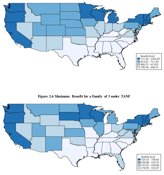
Figure 2.5 Maximum Benefit for a Family of 3 under AFDC . . . 37
Figure 2.6 Maximum Benefit for a Family of 3 under TANF . . . 37
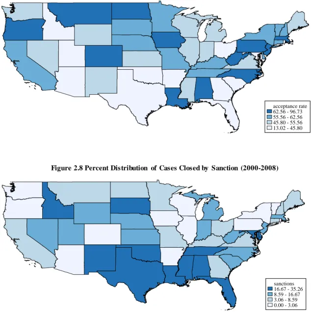
Figure 2.7 Acceptance Rate . . . 38
Figure 2.8 Percent Distribution of Cases Closed by Sanction . . . 38
Figure 2.9 Percent Distribution of Cases Closed by Non-sanction Policy . . . . 39
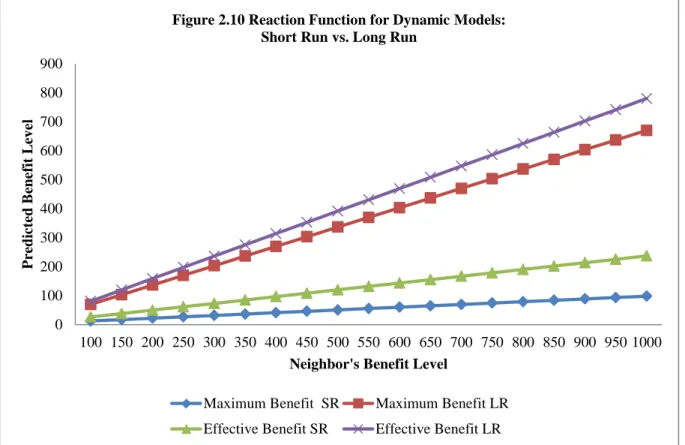
Figure 2.10 Reaction Functions for Dynamic Models . . . 40
Figure 2.11 Poverty Migration Based Weight Matrix . . . 41
Figure 3.1 Life-Cycle Net of Tax Rate by Education . . . 82
Figure 4.1 Coefficient of Variation: Estate Tax Revenue as Percentage of Total State Revenue . . . 118
Figure 4.2 Federal Estate Tax Schedule . . . 118
Figure 4.3 Estate Tax Payable by a $3 million Estate in Pick-up Only State . . . 119
Figure 4.4 Federal Net Estate Tax Collected vs. State Death Tax Credit/Deduction Paid . . . 119
Figure 4.5 Percentage of States Collecting Only the Pick-up Tax . . . 120
1 Introduction
Understanding how economic agents react to changes in the tax and transfer system has long been a topic of great interest to both policy makers and academics. Moreover, given today’s fiscal climate, in which further income tax hikes and cuts to social safety net pro-grams loom in the near future, an enhanced knowledge of such responses will be all the more important. Economists working at the intersection of public and labor economics have devoted much research into identifying behavioral elasticities such as the compen-sated elasticity of labor supply with respect to marginal tax rates and more recently, the elasticity of taxable income. Because elasticities such as these will be inversely related to both the optimal size and progressively of the public sector, pinning them down is crucial for deriving important tax parameters such as the revenue-maximizing rate of taxation for high earners.
Another set of important questions studied by those interested in the design and re-form of our tax and transfer system pertain to matters of fiscal federalism, a subfield of public economics addressing questions related to how to delegate policies among different levels of government. Such questions have been particularly relevant with regards to the nations transfer system given the 1996 welfare reform created by the PRWORA legislation which further decentralized welfare authority to the state governments and the ongoing discussions of how to reform larger programs such as the Supplemental Nutrition Assis-tance Program (SNAP) and Medicaid. The literature on fiscal competition, which studies how decentralized governments respond to policies set in competing jurisdictions (hori-zontal competition) or higher levels of government (vertical competition) has been key to understanding the economic implications of such choices. For instance, the literature has demonstrated how inter-state competition over mobile individuals and capital can theoret-ically lead to a situation sometimes referred to as a ‘race to the bottom,’ in which juris-dictions compete with each other to offer the most attractive fiscal climate and in doing so reach an equilibrium in which taxes (or the generosity of transfer programs) are lower
than they would have been under a centralized system. By examining the behavior of states governments sorrounding past reforms, we can learn much about the strength of inter-state competition and its implications for future policy.
To enhance the body of knowledge relating to the matters discussed above, this disser-tation consists of three essays that focus on identifying the strategic responses of both state level governments and individuals following changes in the tax and transfer system.Two essays contribute to the literature on fiscal competition. Both of which focus on state level polices aimed at redistributing income. A third essay contributes to the literature estimating the responsiveness of individual’s incomes to changing marginal tax rates. As discussed above, a better understanding of these responses contributes to our ability to design an optimal tax and transfer system in a federalist nation. In essay 1 I use a spatial dynamic ap-proach to investigate interstate welfare competition across multiple policy instruments and across three distinct welfare periods - the AFDC regime, the experimental waiver period leading up to the reform, and the TANF era. Results suggest the strategic setting of welfare policy occurs over multiple dimensions of welfare including the effective benefit level and the effective tax rate applied to recipient’s earned income. Furthermore, strategic behav-ior appears to have increased over time consistent with a race to the bottom after welfare reform. Another form of interstate competition is examined in Essay 3 which investigates spatial patterns in state level estate tax policy following a major reform which greatly al-tered both the state and federal estate tax landscape. This study develops a model in which a state’s tax base and rate are simultaneously determined. Results indicate a state’s estate tax base is negatively influenced by its own tax rate and positively influenced by the tax rate set in neighboring jurisdictions. A state’s own tax rate is also found to be positively influenced by the tax rates set in neighboring jurisdictions. Last, Essay 2 uses matched panels from the Current Population Survey for survey years 1980-2009 to estimate the elasticity of taxable income (ETI) and how it varies in response to measurement of the tax rate, heterogeneity across education attainment, selection on observables and unobservable, and identification.
2 Was there a ‘Race to the Bottom’ After Welfare Reform?
2.1 Introduction
The 1996 Personal Responsibility and Work Opportunity Reconciliation Act (PRWORA) abolished the federal entitlement program Aid to Families with Dependent Children (AFDC) and replaced it with Temporary Assistance to Needy Families (TANF), a state administered block-grant program. In doing so, the federal government granted states much greater lat-itude in the design of their respective welfare programs. Leading up to the passage of the reform there was much speculation and debate over the possibility that states would use their new found freedom to “race to the bottom” in setting welfare generosity. Canonical models of fiscal federalism have long suggested that income redistribution, specifically in the form of assistance to the poor, should fall into the realm of responsibility of the federal government (Stigler (1957), Musgrave (1959), Oates (1972)).1 With welfare, it has been ar-gued that decentralized benefit-setting could trigger competition among the states. In such a scenario, policy makers fear that they may attract poor populations from neighboring states, or become a ‘welfare magnet,’ if relatively generous benefits are offered. To avoid this outcome, states may strategically reduce the generosity of their welfare programs and compete with neighbors to offer less desirable benefits.
To gauge the likelihood of this scenario, researchers began looking for evidence of competitive behavior among states before the reform went into effect (Brueckner (2000), Figlioet al.(1999), Shroder (1995), Romet al.(1998), Saavedra (2000a)).2 However, little is actually known about the extent of strategic competition after welfare reform. In effect, the question ‘did welfare reform actually kick off a race to the bottom?’ remains unan-swered. Understanding state behavior following the reform is especially relevant today
1While the mobility of individuals generally leads one to view local governments as constrained in the amount
of redistribution they can carry out, this normative position has not gone unchallenged. Under certain as-sumptions, some have shown local redistribution to be efficient (Pauly (1973), Epple and Romer (1991)).
2The focus of these studies was the AFDC statutory maximum benefit level which was determined at the state
given growing political pressures to further reform the social safety net and specifically the current proposals that would block grant funding and give states more control over addi-tional programs including medicaid and the Supplemental Nutriaddi-tional Assistance Program (SNAP). Using dynamic spatial econometric methods, this paper provides the first evidence on competition after the 1996 reform.
Because of the large array of new policies available to state policy makers (time limits, family caps, sanctions, earnings disregards, etc.), a test of welfare competition that sim-ply extended past methodologies over the TANF era would miss many dimensions over which states could conceivably compete. While the statutory benefit level remains a pol-icy instrument readily available for reform, the water is muddied by the numerous other instruments states now have at their disposal.3 If states have in fact engaged in a “race to the bottom”, it is entirely possible that they did so through more restrictive access, greater policy stringency, or some combination of these and other factors. I extend the literature by utilizing micro caseload data to construct a unique panel of state level welfare policy vari-ables. These include the effective benefit level, the effective tax rate on recipients earned income, state sanction use, and ease of access to benefits. Taken together these variables more fully encompass a state’s welfare policy bundle and the channels through which they might compete.
A second contribution of the analysis aims to more fully understand the evolution of competitive behavior surrounding the reform. Though the PWRORA legislation marked the official transition from AFDC to TANF, implementation was not instantaneous. The two regimes were separated by an experimental period of ‘laboratory federalism.’4 The
3A policy instrument that states do not have at their disposal is the use of any kind of residency
require-ment. The use of such policies has been ruled unconstitutional by the Supreme Court - once under the AFDC regime (Shapiro v. Thompson (1969) and again following PWRORA after fifteen states attempted to implement policies which would pay lower benefits to newcomers (Saenz v. Roe (1999).
4A provision of the Social Security Act, dating back to 1962, permitted the secretary of Health and Human
Services to waive the rules and regulations surrounding AFDC in certain contexts. Specifically, states had the power to petition the U.S. Department of Health and Human Services for such waivers allowing them to implement experimental programs or policies designed to increase program effectiveness(Grogger and Karoly (2005)).
existence of such a period provides a unique opportunity for investigating changes in in-tensity of strategic behavior. Specifically, during the experimental “waiver period,” states had additional policy freedoms but were not yet bound by the new TANF provisions and fi-nancing arrangements. To exploit the changing policy landscape, I analyze strategic policy setting over a twenty-five year window (1983-2008) divided into three distinct periods: the AFDC era (1983-1991); the experimental waiver period (1992-1996); and the post reform TANF regime (1997-2008). Through this division I can test for changes in the intensity of strategic behavior across the different regimes.
Finally, though the importance of dynamics has been recognized in the welfare caseload literature (Ziliaket al.(2000), Haider and Klerman (2005)), the welfare competition litera-ture has largely ignored the importance of dynamics in the determination of welfare policy. To address this matter, I further extend the literature by providing the first dynamic esti-mates of welfare competition. To do so, I adopt a spatial dynamic panel estimator which permits both short and long run estimates of strategic policy setting. The dynamic spec-ification can be rationalized on several grounds. First, there are likely to be lags in the diffusion of information about changes in neighbors’ welfare policy. Second, the political process takes time. States wishing to enact policy changes in response to their neighbors’ policies may not be able to do so immediately. Third, state welfare policies are highly persistent (Ziliaket al.(2000), Haider and Klerman (2005)) and failing to control for last years policies, or state dependence, may lead one to overstate the magnitude of strategic behavior. Through the addition of dynamics, one is provided a better understanding of the importance played by strategic behavior in the determination of state policy over time.
The static model shows that states strategically set welfare policies in conjunction with those of their neighbors. Moreover, this strategic behavior was not limited to the statutory benefit level examined by the past literature. Rather, it spanned multiple policy instruments affecting the effective benefits level and tax rates faced by recipients in each state, con-sistent with competition over the benefit base. Furthermore, it appears strategic behavior
intensified in the waiver and TANF periods. For instance, during the AFDC regime, es-timates suggest states responded to a 10 percent cut in the effective benefit level of their neighbors’ with an own cut of around eight and one half percent. This magnitude increased to nine percent and then nine and a third percent for the waiver and TANF periods, respec-tively. When the models are augmented to allow for asymmetrical policy responses (i.e. states’ responses are conditioned on their relative position to their neighbors), I find that states offering relatively generous policies are more responsive to cuts in generosity by bor-dering states as one would expect in a “race to the bottom” scenario (Figlioet al.(1999)). Furthermore, the three period analysis reveals that the asymmetrical response behavior is concentrated in the waiver and TANF regimes.
Finally, the results demonstrate the importance of modeling welfare competition in a dynamic framework. In terms of importance, lagged own state policy variables clearly dominate those of neighbors for short run policy determination. Spatial coefficients, which capture a state’s reaction to its neighbor’s policies, are reduced in economic importance and in some instances lose statistical significance under the dynamic specification. Most notable is the case of the maximum benefit level. Once controlling for a states’ lagged own maximum benefit level, the maximum benefit level of bordering states no longer appears to exert much influence on state policy choice. However, evidence of strategic policy setting in both the short and long run remains for many of the new variables under consideration, especially the effective benefit level and the effective tax rate on earned income. Long run coefficients suggest that neighbor policy does play an important role in a state’s determina-tion of welfare policy over time. Sensitivity analysis reveals findings are robust to multiple spatial weighting schemes and specification choices.
2.2 Welfare Reform and the “Race to the Bottom”
The PRWORA legislation, now commonly referred to as welfare reform, sought to “end welfare as we know it.” As outlined in Blank (2002), the major reform provisions included
the devolution of greater policy authority to the states, the change in financing, ongoing work requirements, incentives to reduce non-marital births, and a five year maximum time-limit. Of these provisions, the first and second were central to the “race to the bottom” debate.
2.2.1 Greater Policy Authority for the States
Under TANF, states were given increased discretion over eligibility, the form and level of benefits, and the ability to impose even more stringent time limits and work requirements if they so chose (Blank (2002), Grogger and Karoly (2005)). While many of the new policies were designed to force participants to work and punish or sanction those who did not comply, others were implemented to increase the reward to working. Examples of the latter included reduced statutory tax rates on recipient’s income as well as expansions in earnings disregards and liquid asset limits which determined benefit levels and eligibility (Ziliak (2007)). These so called “carrots and sticks” of welfare reform were applied at the discretion of each state and entered into use during the early 1990s in the experimental waiver period.
Waiver-based reforms that had gone largely unused until the 1990s suddenly became a key mechanism in the states’ push for reform. During this time, eighty-three waivers were granted to forty-three states and the District of Columbia (Grogger and Karoly (2005)).5 For example, sixteen states were granted approval to implement various statewide time-limit policies. Of these, Iowa was the first state to receive approval in 1993. Other midwest-ern states to adopt time-limit waivers included Indiana (1994), Nebraska and Illinois (1995) and Ohio (1996). Connecticut implemented the strictest time-limit policy of twenty-one months which applied to the whole family. Delaware, Virginia, and South Carolina also re-ceived approval for strict full family time-limits of twenty-four months. Statewide family-cap waivers were granted to nineteen states between 1992-1996. The majority of these
5The following information on specific state waiver policies is drawn from Chapter 2 of Grogger and Karoly
allowed no increase in benefits for additional children beyond a certain number. Statewide financial-incentive waivers were granted in twenty states over the same period. Before the waiver period, welfare recipients faced a benefit reduction ratio of 100 percent after just four months of working.6 In an attempt to encourage labor force participation or “make work pay,” states experimented with increasing the income disregard and lowering the im-plicit tax rate. Michigan, for instance, allowed a $200 disregard and lowered the tax rate on earned income to twenty percent while Connecticut allowed recipients to keep 100 percent of their earnings up until the federal poverty line. These constitute just a few of the exam-ples of policies states initially enacted during the waiver period and carried over to TANF. Perhaps unsurprisingly given the evolution of U.S. welfare reform, it was not only these new waivers state policymakers pushed for in the final national reform. They also sought the devolution of responsibility in program design from the federal level to the state.
Naturally, some believed this new found flexibility in welfare design would prove ef-ficiency enhancing, as states could now tailor their programs to meet their citizens’ (both tax-payers and potential recipients) wants and needs more closely. Others, however, were concerned that the further decentralization of benefits would have a more worrisome ef-fect – the aggravation of interjurisdictional externalities suggested by the fiscal federalism tradition. While popular usage of the term “race to the bottom” tends to overstate the sit-uation or connote “a draconian tendency to slash welfare benefits to the bare minimum, mimicking the outcome of the least generous state,” the fact remains that economic theory does point to a downward bias in generosity (Brueckner (2000)). This benefit underpro-vision result has been demonstrated in the literature many times. The standard models of benefit competition, built on the work of Brown and Oates (1987), Bucovetsky (1991), and Wildasin (1991) consist of multiple jurisdictions composed of taxpayers and mobile poor non-taxpayers who receive a welfare benefit. The welfare benefit is selected in each juris-diction to maximize the utility of the taxpayers (who care about the poor in their own
ju-6AFDC’s first finical work incentive, known as the “thirty-and-a third” policy, was enacted in 1967 but later
risdiction) taking into account the benefit level in other jurisdictions. First order conditions from these models take on the form of a Samuelson condition for the optimal provision of a public good where the sum of the taxpayers marginal utility gain from increasing the benefit is equal to the marginal cost. The suboptimality of this result is easily demonstrated by obtaining the same condition for the case in which the poor are immobile. Comparison reveals that the marginal cost of raising benefits will be higher when the poor can migrate which leads to a lower benefit level than in the no migration case. Thus decentralized benefit setting is said to lead to benefit under-provision.
To test this prediction, the past welfare competition literature focused on the maximum AFDC benefit guarantee (sometimes augmented to include food stamps) for a given family size. However, this statutory maximum may not sufficiently reflect a state’s welfare policy. Under welfare reform, other critical factors include the rates at which states ‘claw back’ benefits as a recipient’s income increases along with the levels and sources of income that may be excluded from benefit determination formula (Ziliak (2007)). These factors which are determined by state policy act to drive a wedge between the statutory maximum benefit level and the prevailing average effective benefit. This can be demonstrated with the stan-dard benefit determination formula denoted as:B =M B−brr∗(W H+N −D), where MB is the maximum benefit guarantee, brr is the states benefit reduction ratio (which was set at 100 percent under AFDC), WH is labor income, N is any non-labor income, and D is the earnings disregard). Prior to the reform many states did implemented earnings disre-gards which led to effective tax rates of less than 100 percent. However, they were bound by the statutory benefit reduction rate of 100 percent. During the waiver period and follow-ing TANF, many states set new benefit reduction rates and earnfollow-ing disregard policies. For instance, Michigan and Maryland implemented a benefit reduction rate of only twenty per-cent during the waiver period while rates of twenty-five perper-cent, thirty-three perper-cent, and fifty percent were set in place by Vermont, California, and New Hampshire, respectively.
average statutory maximum and average effective benefit level for a family of three.7 For both variables a clear downward trend emerges in the late 1980s, which is consistent with welfare competition. Even more interesting is the divergence between effective and statu-tory benefit guarantees whose onset coincides with the 1996 reform. Ziliak (2007) notes that the falling effective guarantees make welfare less attractive and are in line with the reform goals of encouraging work and discouraging welfare use. One could also speculate that these falling effective guarantees are consistent with states’ strategic efforts to keep their welfare programs from appearing to be more desirable than their neighbors. Though the effective benefit level may better reflect a state’s generosity relative to the statutory maximum, the picture is not complete until one considers the effective tax rates faced by recipients. The effective tax rate on earned income reflects the rate at which a state reduces the monthly benefit amount paid to recipients as they earn labor income. State policies such as reduced statutory rates and earnings disregards, lower the effective rate of taxation and thus increase both the level of generosity and work incentives. Before the reform, this tax rate had a statutory value of 100 percent though in practice it was much lower and displayed a considerable degree of cross-state heterogeneity (Lurie (1974), Hutchens (1978), Franker
et al.(1985), McKinnish (2007a)). After the reform, the rates fell rapidly as seen in Figure 2.2 A strong case can be made for the use of these ‘effective’ variables. Though they can-not separately identify the individual policies, these variables will reflect a states’ collective use of policies such as family caps, asset limits, partial sanctions and earning disregards, as well as caseworker discretion in the application of these policies (Ziliak (2007)).
However, there is also an extensive margin of generosity to consider. States can set strict eligibility criteria, harsh sanction policies, or shorter more restrictive time limits. Three additional measures therefore aim to capture aspects of state policy not represented by the benefit and tax rate instruments discussed above. The first is the approval rate which is meant to proxy for ease of access to welfare benefits. The latter two reflect a state’s
strin-7The effective benefit variable is constructed using administrative micro caseload data from the AFDC
gency in terminating cases through the use of sanction and other non-sanction state polices (such as shortened time limits). These measures are constructed using micro caseload data available only for the post-reform regime. Figure 2.3 illustrates a national trend towards declining case approval rates coinciding with an increasing trend in case termination due to sanctions. Specifically, average state case approvals fell approximately seventeen percent between 2000 and 2008 while sanction use nearly doubled. Overall, the trends documented here suggest a tendency towards reducing welfare generosity along multiple margins con-sistent with a race to the bottom. Detailed information on the construction of all variables and their sources are provided in the data section.
The additional policy autonomy for the states was not the only factor cited in the grow-ing debate on whether states would “race to the bottom.” Critics of the reform also argued that the new cost-sharing arrangement between states and the federal government would exert further downward pressure on benefits.
2.2.2 Change in Federal Cost Sharing
Brueckner (2000) demonstrated that a price correction mechanism, such as a system of matching grants with the federal government, can be used to decrease the price of addi-tional welfare spending and restore benefits to their optimal level. Such a system was in existence prior to PRWORA. The reform, however, replaced this cost-sharing scheme with a block grant system. With the old system of open-ended matching grants, states would share any increase in their costs with the federal government (sometimes with the federal government footing as much as eighty percent of the bill).8 Under TANF, states receive a lump sum block grant which was initially tied to the level of federal matching-grant pay-ments a state received in 1994 (Brueckner (2000)).9 As noted in Romet al.(1998), each
8Under AFDC, the federal matching rate for each state was calculated based on the state’s per capita personal
income (PCI). The specific formula, match rate= 100−.45∗ (StateP CIU.S.P CI)2, was the same formula used to determined the Medicaid matching rate and was designed to give relatively poorer states more federal assistance.
9The amount of the block grants was not tied to inflation. Between 1997 and 2011, the value of these grants
state therefore bears the full marginal cost of any increased spending in its welfare pro-gram. Alternatively, states gain the full marginal benefit of any cost savings they incur. In such a setting, attracting welfare migrants from low-benefit states would be quite costly, and more so than before. Consequently, it was suggested that welfare competition could intensify post reform, speeding up the race to the bottom (or at least the race to the benefit floor required by federal law). Policy makers, perhaps in anticipation of strong downward pressure on benefits levels, set “maintenance of effort” requirements stipulating that states may not spend less than eighty percent of what they spent in 1994 (or seventy-five percent if they meet minimum work requirements).10
While theory suggests the move towards greater state policy authority and block grant financing could have led states to underprovide or even “race to the bottom” in setting their welfare generosity, assessing the importance of any resulting competitive behavior is an empirical matter.
2.2.3 Empirical Tests of “Race to the Bottom”
Because welfare migration is held to be the key mechanism in race to the bottom theory, initial empirical studies sought to test whether or not migration actually occurred at any meaningful magnitude. However, these studies found rather mixed results.11 The lack of conclusive results confirming welfare migration does not prima facie rule out race to the bottom behavior. As explained by Brueckner (2000), if state governments merely perceive generous welfare benefits to attract welfare migrants, then the requirements for strategic interaction and the resulting race to the bottom are met. He therefore argues, “because it focuses directly on the behavioral response that leads to a race to the bottom, which may arise even if welfare migration is mostly imaginary, a test for strategic interaction may be more useful than a test for migration itself.”
10Like the block grants, MOE requirements were not indexed for inflation and have thus greatly declined.
11See Brueckner (2000) for a survey covering empirical studies of welfare migration. More recent works
The canonical approach is to employ a fiscal reaction function that relates the welfare benefit level in one state to the benefit level in surrounding states, conditional on a state’s socioeconomic conditions (the poverty rate, female unemployment rate, state per capita personal income, population, governor’s political party, etc.). Equation (1) represents the typical model,
bi =φ X
j6=i
ωijbj +Xiβ+εi (1)
Herebi represents the benefit level in state i, whilebj is the benefit level in all other states j, wherej 6=i. Xi is a matrix of controls for state i,β, its accompanying coefficient vector, andεi is an error term. The weights, or importance, state i attaches to the benefit levels in other states make up theωij vector. Lastly,φis the parameter representing the slope of the reaction function. This parameter will take a non-zero value in the presence of strategic interaction.12
To estimate equation (1) an a priori set of weights that determines the pattern of inter-action between state i and their neighbor’s must be specified. Consequently, the question as to which states should be considered neighbors is an important one. In related literatures investigating strategic tax and expenditure policy setting, “economic” neighbors (which are not necessarily geographic neighbors) have been defined based criteria such as racial com-position or income (Case et al.(1993)). However, because welfare migration (or the fear of welfare migration) is the main factor behind strategic interaction, it is natural to assume a state will be most concerned with the policies of their geographic neighbors - arguably more so, than in related literatures when strategic interaction is driven by capital mobility.13 Therefore, my initial weight matrix, WI, is a simple contiguity matrix where each state as-signs a weight of zero to noncontiguous states(ωij = 0)and equal weights (ωij = 1/ni)
12Strategic interactions can be explained by behaviors such as welfare competition, yardstick competition, or
policy copycatting among states.
13Saavedra (2000) argued that a state will be more fearful of attracting welfare migrants from nearby states
to bordering states whereni is the number of states contiguous to i. Because one’s geo-graphic neighbors remain unchanged, the weights for each state will be time invariant. All baseline models are estimated with this simple weighting scheme. Weighting schemes in which a state scales the importance they attribute to neighbors based on population flows and distance are explored in the sensitivity analysis and discussed therein.
Because benefit levels in different states are believed to be jointly determined, the inclu-sion of benefit levels on the right side of equation (1) creates an endogeneity problem that must be addressed in estimation. Common methods include reduced form estimation using Maximum Likelihood (ML) spatial econometric techniques and an instrumental variable approach. Past studies of AFDC benefit competition employing the reduced form approach include Saavedra (2000) and Rom et. al (1998).14 Both author’s estimate versions of what has become known in the literature as the spatial lag model with some key distinctions. Specifically, Saavedra’s model is adopted to allow errors to follow a spatially autocorre-lated process and is applied to several cross sections (1985, 1990, and 1995). Romet al.
(1998) use a panel of data covering 1976-1994. They include a temporal lag of AFDC benefits among their control variables in order to address contemporaneously correlated errors but do not take into account spatial error correlation.15 In both studies, estimates of
φ, the slope of the reaction function are positive and statistically significant. One drawback with this type of econometric approach is the need to impose restrictions on the reaction function’s slope parameter.16 Another is the fact the ML spatial methods require the inver-sion of the spatial weight matrix which can be computationally demanding (Kukenova and Monteiro (2009), Kelejian and Prucha (1998), Lee (2007)).
14This method requires inverting the model given by (1). Specifically, one takes the matrix form of (1) given
byB=φW B+Xβ+and solves for B which yields the reduced form equationB= (I−φW)−1Xβ+
(I−φW)−1ε. The equation can then be estimated using ML techniques assuming(I−φW)is invertable.
15Under the reduced form approach, failing to account for spatial error correlation can result in spurious
evidence of welfare competition. The inclusion of the lagged dependent variable introduces further econo-metric issues which are not addressed in Romet al.(1998) but are in the current paper.
16Consistent and efficient estimation of model parameters with MLE requires the structure of the interaction
given by the product ofφand W in the reduced form model to be nonexplosive. In the usual case,φmust be less than one in absolute value.
Figlio et al. (1999) use a two-stage IV approach to investigate the extent of strategic interaction present among states over the period 1983 to 1994.17 Neighbor’s benefits are instrumented with the weighted average of a subset of neighbor covariates, a common ap-proach in the literature. Substantial evidence in favor of strategic benefit setting is found. Evidence of asymmetric responses to changes in neighbors benefits levels are also found. Specifically, states appear to respond much stronger when neighbors cut benefits and less so when they increase them. Evidence of benefit competition has not been limited to the U.S.. Using similar methodologies Dahlberg and Edmark (2008) and Fiva and Rattsø (2006) find evidence consistent with a race to the bottom in Swedish and Norwegian municipalities respectively. See Figure 2.4 for details regarding the weighting schemes, data choice, es-timation technique and findings for these past benefit competition studies. In addition to the studies included in Figure 2.4, Shroder (1995), Berry et al. (2003), and Bailey and Rom (2004) also addressed the question of interstate welfare competition using somewhat different econometric approaches. Of these studies, Bailey and Rom (2004) is the only to produce strong evidence of strategic welfare competition.
2.3 Estimation Issues
As previously discussed, the welfare competition literature has largely ignored the impor-tance of dynamics in the determination of welfare policy. In part, this is likely due to the fact that spatial estimators capable of providing proper econometric treatment to both an endogenous spatial term and a lagged dependent variable have only recently become avail-able. Also, some of the initial tests for welfare competition which sought to sign the slope of the theoretically ambiguous reaction functions were preformed with cross sectional data. However, because a states welfare policies are likely as much a function of time as they are of space, a dynamic framework is required to identify the importance of strategic
interac-17While two-stage IV methods may be inefficient relative to ML methods, they have the advantage of being
computationally simpler and avoid strong assumptions on the normality of the error term (Lee (2007)). Also IV produces results which are robust to the presence of spatial error correlation.
tion in the determination of state welfare policies.
This analysis implements a dynamic estimator new to the welfare competition litera-ture. Specifically, I use the generalized method of moments (GMM) estimator proposed by Blundell and Bond (1998) that has become increasingly popular in the empirical literature dealing with spatial dynamic panel models with several endogenous variables.18 I begin with a basic empirical model of strategic interaction similar to those previously discussed augmented to include a lagged dependent variable.
Yit =γYit−1 +φ 48 X
i6=j
ωijtYjt+Xitβ+αi+δt+εit (2)
HereYitrepresents each of the six welfare policy instruments under investigation for state i in time t.Yjtrepresents these policies in all other states j at time t, wherej 6=i. State fixed effects, time effects, and the i.i.d error term are denoted byαi,δt, andεitrespectively. The importance or weight assigned to state j by state i at time t(j 6=i)is represented byωijt.
Note that the static model given by equation (1) is embedded within this equation when
γ = 0, or a state’s lagged policies are not included in the model. With the dynamic model given by (2), one can obtain estimates of strategic policy setting for both the short and long run. The estimate of strategic policy setting over the short run is given by the coefficient,
φ, while the long run coefficient is calculated using the short-run coefficient and the coef-ficient on the lagged dependent variable. Specifically, the long run coefcoef-ficient is equal to
φ 1−γ.
19 Estimates of the short run coefficient,φ, capture the magnitude of a state’s immedi-ate policy reaction to those of its neighbors while long run coefficients capture the policy adjustment process. Consequently, differences between the short and long run estimates
18Kukenove and Monteiro (2009) and Jabobs et al. (2009) both consider the extension of the Blundell Bond
(1998) estimator for the estimation of models with spatially lagged dependent variables. Monte Carlo sim-ulations show the estimator performs well in terms of bias and RMSE and that the system GMM estimator outperforms the Arrelano and Bond difference estimator. Papers applying the System GMM estimator
to spatial panels include Madariaga and Poncet (2007), Foucaultet al.(2008), Wren and Jones (2011),
Bartolini and Santolini (2011), and Neumayer and de Soysa (2011).
19Standard error for the long run coefficient are obtained using Stata’s nlcom command. Calculations are
will be governed by the degree of policy persistence given by the parameterγ.
In order to remove the fixed effects (αi) which are correlated with the covariates and the lagged dependent variable, equation (3) is first differenced and rewritten as:
∆Yit=γ∆Yit−1+φ∆ 48 X
i6=j
ωijtYjt+ ∆Xitβ+ ∆δt+ ∆εit (3)
Though the data transformation removes the fixed effects, the lagged dependent variable remains endogenous since the term Yi,t−1 included in ∆Yit−1 = Yi,t−1 − Yi,t−2 is corre-lated with theεi,t−1 in∆εit = εit −εit−1. So too does the neighbor’s jointly determined policy. Finally, any predetermined covariates in X become potentially endogenous given that they too may correlate with εi,t−1. Following the GMM procedure, one can instru-ment endogenous regressors with deeper lags which remain orthogonal to the error. Under the assumption that error term is not serially correlated, valid moment conditions for the endogenous variables are given by conditions (4)-(6)
E[Yi,t−τ∆εit] = 0; f or t= 3, ...T and2≤τ ≤t−1 (4)
E[Wi,t−τYi,t−τ∆εit] = 0; f or t= 3, ...T and2≤τ ≤t−1 (5)
E[Xi,t−τ∆εit] = 0; f or t = 3, ...T and1≤τ ≤t−1 (6)
Conditions (4) and (5) restrict the set of instruments for the change in own lagged policy,
∆Yi,t−1, and the change in neighbor’s policy,∆P48i6=jωijtYjt, to levels of their second lags
or earlier. Condition (6) requires predetermined covariates be instruments with their first lags or earlier. Because lagged levels of variables can be weak instruments when a variable is highly persistent (as is the case with the welfare variables), the system estimator of Blundell and Bond (1998) adds the original levels equation given by (2) to the model with the additional moment conditions:
E[∆Yi,t−τεit] = 0; f or t= 3, ...T (7)
E[∆Wi,t−τYi,t−τεit] = 0; f or t= 3, ...T (8)
E[∆Xi,t−τεit] = 0; f or t= 2, ...T (9)
The regression in levels given by equation (2) and the regression in differences given by (3) are combined into a system and estimated simultaneously with lagged levels serving as instruments for the difference equation and lagged differences serving as instruments for the levels equation in accordance with the moment conditions (4)-(9). The model is estimated in natural logs allowing coefficients to be interpreted as elasticities.
The consistency of the GMM estimator will depend of on the validity of the instruments. However, under the above moment conditions, the instrument count grows prolifically in T creating problems in finite samples (Ziliak (1997)).20 To avoid these problems I follow Kukenova and Monteiro (2009) and Jacobs et al. (2009) and collapse the instruments.21 Collapsed moment conditions differ from the those proposed in Arellano and Bond (1991) where each moment applies to all available periods rather than a particular time period. For instance, under this modification the moment condition given by (4) now appears as
E[Yi,t−τ∆εit] = 0; 2 ≤τ ≤t−1 (10)
The new conditions still impose orthogonality, but now the conditions only hold for eachτ
rather than for each t andτ.Collapsed instruments can be shown to lead to less biased esti-mates but their standard errors tend to increase (Roodman (2006)). Two specification tests are conducted to verify the validity of the chosen instrument set. Specifically, the Hansen
20 The use of too many instruments will over fit an endogenous variable and result in poor estimation of
the optimal weighting matrix. Roodman(2009) notes it is not uncommon for the optimal weight matrix to become singular and force the use of the generalized inverse.
21Collapsed instruments have also been used in the economic growth literature where dynamic panel models
of a similar cross-sectional and time dimensions are estimated. See for instance Cauldron et. al (2002), Beck and Levine (2004), and Karcovic and Levine (2005).
test for over identification is performed to verify instrument validity while the Arellano-Bond test is performed to verify the the required assumptions on the absence of serial correlation in the level residuals. The system estimator described above is used to obtain estimates ofφ, the reaction function slope parameter, for each of the six policy instruments across the full sample period (1983-2008) and the three distant welfare periods - the AFDC regime, Waiver period, and TANF era.
2.3.1 Allowing for Asymmetrical Policy Responses
The idea that a state may respond differently to the policies of their neighbor’s given their neighbor’s policy action (i.e. benefit increase versus benefit cut) or their relative position (relatively generous or relatively stingy) has taken hold in the welfare and more general fis-cal competition literature (Figlio (1999), Bailey and Rom (2004), Fredriksson and Millimet (2002)). The premise has a clear intuitive appeal for researchers attempting to disentangle whether competition or some other competing explanation (yardstick competition, copy-catting, common intellectual trend) is driving the strategic policy behavior. Under the “race to the bottom” scenario one could expect a benefit cut by one state to invoke a larger policy response from neighbors offering relatively more generous benefits than neighbors who al-ready have a low benefit level. I therefore extend the model to allow for asymmetrical state responses. Specifically, equation (2) is written as
Yit =γYi,t−1+φ0Iit 48 X i6=j ωijtYjt +φ1(1−Iit) 48 X i6=j ωijtYjt+Xitβ+αi+δt+it (11) where Iit= 1 if Yit > P i6=jωijtYjt 0 otherwise
In doing so, I allow states to be differentially impacted by the changing welfare policies of their neighbor’s conditioning on whether their benefits, tax rates, etc. are above or below the weighted average of their neighbors. Under this specification,φ0 (φ1) gives the strategic response of states with welfare policies higher (lower) than the weighted average of their neighbors. Wald tests are utilized to determine if response asymmetries are present. Under the null hypothesis,φ0=φ1, state’s respond the same to a neighbor’s policy change regardless of their relative position. Rejection of the null hypothesis is consistent with response asymmetries.
2.4 Data
To estimate equations (2) and (11), I assemble a panel of data on state welfare policies, demographics, and the macro economic and political environment for the years 1983-2008. For the maximum benefit level I use the state set maximum AFDC (or TANF) benefit level for a family of three collected from the UKCPR’s welfare database.22 To obtain state level estimates of the effective benefit guarantees and tax rates, I implement the reduced-form methodology of Ziliak (2007) which requires the use of administrative micro caseload data.23 With such data one regresses the actual AFDC/TANF benefit for recipienti = 1, ...N, in statej = 1, ...J,at time t = 1, ...T on the recipient’s earned in-come, unearned/transfer income and controls for the number of children. State specific and time-varying intercepts combined with coefficients on variables indicating the presence of additional children provide an estimate of the effective benefit guarantee for families of various sizes. The coefficient on the recipients earned income is used to provide esti-mates of effective tax rates.24 The caseload data used in constructing these estimates comes from two different administrative sources. The first is the AFDC Quality Control System
22www.ukcpr.org/AvailableData.aspx
23I am grateful to Jim Ziliak for providing programs and data which allowed me to replicate and extend his
1983-2002 analysis through 2008.
24A more detailed explanation of the construction of the effective benefit guarantees and tax rates is contained
(AFDC-QC), which covers 1983-1997, and the second is the National TANF Data Sys-tem (NTDS), which covers 1998-2008.25 Summary statistics for the benefit and tax rate variables are presented in Table 2.1 for the pooled sample and the three separate welfare periods. The geographic distribution of benefit levels is illustrated by Figures 2.5 and 2.6 which map the maximum state benefit levels for the AFDC and TANF periods. Looking at 2.5, the AFDC map, one can see a clear pattern of geographic clustering with the most generous benefits levels located in the New England and west coast and the least generous located in the south. Moving to 2.6, the TANF map, one can see the map lighten as more states join the lower benefit levels.
The final three welfare measures are constructed from data available only for the TANF period. The first of these is the approval rate which I define as the average monthly num-ber of applications approved over the average monthly applications received.26 The other two variables capture state strictness in removing people from the welfare roles. The first, sanction use, is defined as the percent distribution of TANF closed-case families with cases closed by sanctions. The final variable, non-sanction state policy, is defined as the per-cent distribution of TANF case-closed families with cases closed by state-policy. Case closure data comes from the Characteristics and Financial Circumstances of TANF Recip-ients database.27 Summary statistics for these variables are presented in Table 2.1. Their geographic distributions are displayed in figure 2.7-2.9. From the map, one can tell some states - Idaho, Texas, Florida, Oklahoma, and Maryland, for example - appear very policy stringent by displaying both low access rates and high sanction use. Other states, New York, Pennsylvania, Utah, and Oregon, among others, appear more lenient with higher acceptance rates and very low sanction use.
25The NTDS is called the Emergency TANF Data System for the years 1998 and 1999. See Ziliak (2007) for
a detailed discussion of the micro data and sample selection criterion. The AFDC-QC data and codebooks for 1983-1997 are available online at http://afdc.urban.org/ while the TANF 1998-2008 data are available online at http://aspe.hhs.gov/ftp/hsp/tanf-data/index.shtml
26The application data is available online for the years 2000-2010 at
www.acf.hhs.gov/program/ofa/data-reports/caseload/applications/application.htm
The control variables adopted for this analysis are those commonly found in the em-pirical literature and are meant to capture aspects of each state’s economic and political climate as well as characteristics of the low-skill and female labor market. Specifically I control for population, the African American proportion of the population, the poverty rate, the female unemployment rate, median wage, employment per capita, and an indica-tor for a democratic governor. The African American proportion of the population, median wage, and female unemployment rate are constructed from the Current Population Survey (CPS).28The remaining variables come from the UKCPR’s welfare database. All variables are measured in 2007 dollars. Descriptive statistics are presented in Table 2.1.
2.5 Results
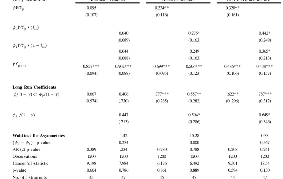
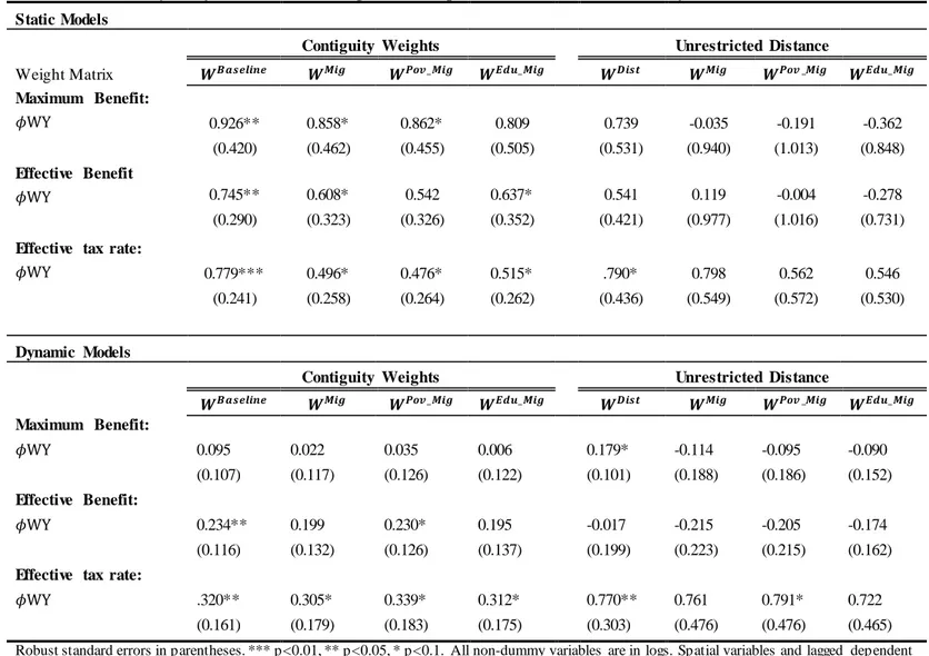
All models are estimated in both a static and dynamic framework. I begin by presenting the results for the benefit and tax rate variables over the full 1983-2008 period and then the three separate welfare periods - AFDC, waiver, and TANF. Results for the remaining variables (access, sanctions, and non sanction state policy) are reported separately as they span a different time period (2000-2008). I report models with and without allowing for response asymmetries. W Yp denotes the spatial coefficient in the model without asym-metries, where different policy instruments are indexed by p. For the model including asymmetries,W Yp(Iit)denotes the spatial coefficient for states with benefits, tax rates, etc. greater than their neighbors on average, whileW Yp(1−Iit)is the response of states setting these policies lower than their neighbors on average. Wald tests are presented to indicate whether or not response asymmetries are present. Hansen tests for over identification are presented for all models and consistently fail to reject the null of valid instruments. The Arellono-Bond tests for serial correlation and instrument counts are also reported.
The baseline models use the main contiguity weight matrix, WI. Endogenous spatial variables are instrumented with their second through fourth lags collapsed in all initial
28To address the fact that samples sizes can be limited for subpopulations in smaller states, these variables
models while controls are treated as predetermined and instrumented with their first lag collapse.29 Estimates of control variables are suppressed for ease of presentation. Full results are available upon request.
2.5.1 Static Results
Table 2.2 presents the full period analysis. Evidence of strategic state policy setting is found across all benefit and tax rate variables for the 1983-2008 period. Estimates of the different spatial coefficients are both economically and statistically significant. The mag-nitude of strategic behavior appears to be largest for the maximum and effective benefit levels. Estimates suggest that states respond to a 10 percent cut in the average benefit level of the their neighbors with an own cut of around 9.3 percent. When allowing for asymmet-ric responses, I find states are slightly more responsive to cuts in neighbors benefits when their own benefit level is above the weighted average of their neighbors.30 Though not conclusive evidence, the finding of asymmetries suggests the strategic interaction found is likely due to competitive behavior rather than other phenomenons noted in the literature (yardstick competition, copy-catting, common intellectual trend) or some geographically correlated omitted variable. Or, as stated by Figlio et. al (1999), it appears that “states are more concerned about being left-ahead in welfare benefit levels than they are about being left behind.” Strategic policy setting over the effective benefit level is also detected and indicates states respond to a 10 percent cut in neighbor effective benefits with an own cut of 7.5 percent Evidence of competition over the effective benefit suggests states could be strategically using polices such as family caps, partial sanctions, and financial incentives to keep the actual benefits they pay in line with their neighbors. This finding implies there
29Estimates are robust to the use of multiple lag structures (see sensitivity analysis located in appendix). 30Asymmetry results for the benefit level variables do not produce much of a differential affect and are
therefore not of much interest. However, more important asymmetries are detected for the remaining policy instruments. It is also worth noting that while one might expect the main estimate of the spatial coefficient to provide a upper bound (or lower bound) for states below the mean (above the mean), this is not always the case or required econometrically given the time varying nature of whether a state falls above or below the mean.
may exist competition over the benefit base as well as the level. Moving onto the tax rate results, I find that a 10 percent cut in the effective tax rate on earned income by states’ neighbors is met with an own state reduction of approximately 8 percent.
Interestingly, the asymmetrical responses to neighbors’ effective tax rates on earnings are much larger and economically important than those found for benefits. While at first one might suspect states engaged in competition would increase effective tax rates in order to reduce overall generosity, this is not necessarily the case.31 Cuts in the effective tax rates coinciding with falling benefits would not do much to increase overall state welfare generosity (especially if one was not working or receiving non-labor income). Instead, one should view the falling effective tax rates on earned income as use of ‘carrot’ policies by states to lure recipients to the labor market and eventually off welfare. In some sense, the results suggest states are ‘racing to force recipients back to work’. A state that finds itself employing an effective tax rate on earned income greater on average than its neighbors, will match a 10 percent cut in neighbors benefits with a own cut of roughly 9 percent. However, if that same state was instead employing an effective tax rate lower than its neighbors, it will only match a 10 percent cut with and own cut of 6.7 percent. Put another way, while states may ‘race along’ with their neighbors in promoting work, they slow at the prospect of leading this race or being overly generous.
Table 2.3 and 2.4 present results for the three separate welfare regimes. While the full period analysis established evidence of competitive behavior, results produced for this pe-riod could mask changes in state behavior occurring after the onset of the waiver pepe-riod or the 1996 structural shift in the welfare system. For both benefit variables, evidence of com-petition is found across all three periods. Point estimates suggest benefit comcom-petition grew stronger over waiver and TANF periods. For instance, during the AFDC regime, estimates suggest states respond to a 10 percent cut in the maximum benefit level of their neighbor’s with an own cut of nearly 7 percent. This magnitude increases to roughly 9.5 percent , and
31Falling effective tax rates appears to be the dominant trend in the data making a discussion of “race to the
8.7 percent for the waiver and TANF periods, respectively. However, when coefficients are tested for equality across periods, I fail to find evidence that they are statistically different from one another. Interestingly, when asymmetries are included, evidence of asymmetrical responses for the maximum benefit level is only found during the TANF era. The effective benefit displays a very similar pattern with asymmetrical responses detected in both the waiver and TANF regimes. With the effective tax rate on earned income, evidence of com-petition is only found for the AFDC and TANF era. The finding that states implemented very similar tax rates to those of their neighbors under AFDC is perhaps unsurprising given that all states were subject to the same statutory tax rates under this regime. Differentials in state effective tax rates arose primarily due the differences in sources and levels of income disregards permitted by each state. With the onset of the waiver period, states began to experiment by altering their statutory rates and offering further financial incentives. The estimate of strategic policy setting for this period suggests that they did so at first without paying much attention to the policies of bordering states. However under TANF it appears state’s did strategically set policies impacting their effective tax rates. Furthermore, the evidence of important asymmetrical responses are only found for the TANF era. These finding suggests several things. First, my previous findings of behavioral asymmetries for the full period were most likely driven by the waiver and TANF periods. Second, after welfare reform, states appear to place more importance on their relative position to their neighbors as one might expect if competition was intensifying.
Table 2.5 presents the results for the final three welfare variables - ease of access, sanc-tion use, and non-sancsanc-tion state policy. Again, these variables are meant to proxy policy dimensions not captured by the four main policy instruments and are only analyzed for the TANF period. States appear to exhibit strong behavioral responses to their neighbors’ approval rates or ‘ease of access’ to welfare benefits. Specifically, in the model without asymmetrical responses, it appears a state reacts to a 10 percent cut in the weighted aver-age of their neighbors approval rate with an own cut of nearly 8 percent. Setting restrictive