How Far from Kronecker can a MIMO Channel be? Does it
Matter?
Proceedings of European Wireless (EW)
27-29 April, Vienna, Austria, 2011
NAFISEH SHARIATI AND MATS BENGTSSON
Stockholm 2011
Signal Processing
School of Electrical Engineering
Kungliga Tekniska Hgskolan
IR-EE-SB 2011:012
How Far from Kronecker can a MIMO Channel be?
Does it Matter?
Nafiseh Shariati and Mats Bengtsson
School of Electrical Engineering ACCESS Linnaeus Center KTH Royal Institute of Technology
Stockholm, Sweden
Email: [email protected], [email protected]
Abstract—A common assumption in the design and analysis of many MIMO transmission schemes is the so-called Kronecker model. This model is often a crucial step to obtain mathematically tractable solutions, but has also been criticized for being unrealis-tic. In this paper, we present a numerical approach to determine a channel whose statistics is as far from being Kronecker as possible, keeping only an assumption of spatial stationarity. As a case study for the relevance of the Kronecker assumption, a numerical analysis is included of the performance of optimal pilot design for Kronecker and non-Kronecker channels. The numerical results indicate that for this particular application, the Kronecker assumption may be used in the algorithm design and provide performance that is close to optimal also for non-Kronecker channels.
I. INTRODUCTION
The performance of multiple-input multiple-output (MIMO) systems highly depends on the characteristics of the channel over which the radio propagation occurs. Therefore, modeling a dynamic MIMO channel accurately is crucial in system de-sign, not only for numerical simulations but also in the design and analysis. Several analytical models have been proposed for MIMO channels [1]–[3]. A popular choice is the Kronecker model introduced and developed in [1], [4], [5], which assumes independent statistics of the spatial properties, at transmitter and receiver sides. This model has been criticized for not being representative of real-world conditions and for providing inaccurate estimates of the channel capacity [3], [6], see also [7], where the author provides mathematical and propagation conditions for the validity of the Kronecker structure. The authors in [8] also compare the Kronecker model with full geometry-based statistical channel models. In spite of these deficiencies, the model is commonly used in algorithm analysis and design [1], [9]–[11], since it provides analytical solu-tions to problems that otherwise would be mathematically intractable. An engineering approach is then to apply the resulting algorithm also in scenarios where the assumption not necessarily holds. To our knowledge, very few results have been published on the resulting performance of such a strategy. In order to make such a study as trustworthy as possible, it is interesting to find examples of channels that are as far as possible from being Kronecker.
In this paper, we propose a method to find a MIMO channel covariance matrix with maximum mismatch compared to a
given Kronecker structure. The method is based on a semidef-inite relaxation followed by a randomization procedure. An alternative approach appeared in [12] for2×2 channels.
As a case study, we present a numerical performance analysis of optimal pilot signal design, where closed-form solutions were obtained in [11], [13] under the assumption of Kronecker structures both for the channel and also for the spatio-temporal properties of the noise, whereas the pilot design problem in the general case is non-convex. Also, in [14] a closed form solution has been derived under a more general statistical channel model which conveys the Kronecker model as a special case. In the numerical evaluation, we compare using the solution of [11] with a solution obtained using standard non-linear optimization, for channels with different levels of mismatch to the Kronecker assumptions.
The organization of the paper is as follows. Section II is devoted to the Kronecker model and the proposed algorithm to find the worst Kronecker mismatch. Section III provides a brief overview of the pilot design problem which is followed by the numerical evaluations in section IV.
Some notations used throughout the paper are as follows. Bold-face uppercase (lowercase) characters are used for matri-ces (vectors). We useE[·] to denote the expectation operator, Tr[·]the trace operator, and vec(·)the vec operator. The Frobe-nius norm is specified byk · kF, and the Kronecker product by
⊗sign. We also denote transpose and conjugate (Hermitian) transpose of a matrix by (·)T and (·)H, respectively, and
scalar conjugation by (·)∗
. Furthermore, CN(µ,R) denotes symmetric complex Gaussian random variables with mean µ and covariance matrixR.hij denotes the entry in theith row
andjth column ofH.
II. KRONECKERMODEL ANDWORSTCASEKRONECKER
MISMATCH
We consider a narrowband point-to-point multiple-antenna system with nT transmit and nR receive antennas, which is
modeled as
y(t) =Hx(t) +n(t), where x(t) ∈ CnT
and y(t) ∈ CnR
are the transmitted and received signals, respectively, and n(t) ∈ CnR
is the interference plus noise. The MIMO channel H ∈ CnR×nT
If we consider the analytical Kronecker model to describe the MIMO channel, then the channel covariance matrix can be fully determined byR=RT
tx⊗Rrx, whereRtxandRrxare
the correlation matrices at the transmitter and receiver sides, respectively.
One condition for the Kronecker model to hold is that of spatial stationarity, i.e., the correlation coefficients remain invariant to small dislocations of the antennas, as long as the antenna separation at each end remains constant. Therefore, considering uniform linear arrays, the channel correlation
E[hklh∗mn]will be a function of the integer pair(k−m, l−n).
Further, we will assume the channel to be normalized so that the average energy of each channel coefficient is one, i.e., Tr[R] =nrnt.
Define the transmit and receive side correlation matrices as
Rtx= E[H HH] Tr[Rrx] Rrx=E [HHH] Tr[Rtx] ,
and note that these matrices contain values of E[hklh∗mn]
where k = m or l = n, respectively. This means that most elements of R will be directly determined if Rtx and
Rrx are known. Only K = 2(nT −1)(nR−1) parameters,
corresponding tok6=m andl6=n, remain to be determined to completely describe the full matrix R.
One way to determine the remaining parameters is the so-called Kronecker assumption, where the correlation between two elements of H is the product of the correlations as seen from the transmit and receive sides, respectively, i.e.
R=RTtx⊗Rrx,Rkron.
Here, in contrast, we will only use the constraint that R should be a covariance matrix, i.e. that it should be positive semidefinite.
An example of this structure for the case of2×2 channels is provided in [7], [12]. Here, we use the 3×3 case for illustration. The two 3×3 Hermitian matricesRtx andRrx
have the form
Rtx= E [HHH] Tr[Rrx] = 1 t∗ T∗ t 1 t∗ T t 1 , Rrx= E[ HHH] Tr[Rtx] = 1 r∗ R∗ r 1 r∗ R r 1
Assuming spatial stationarity, the full channel covariance
matrix will have the form R=E[vec(H)vec(H)H] = t x6 x5 T x2 x1 Rrx x7 t x6 x3 T x2 x8 x7 t x4 x3 T t∗ x∗ 7 x ∗ 8 t x6 x5 x∗ 6 t ∗ x∗ 7 Rrx x7 t x6 x∗ 5 x ∗ 6 t ∗ x8 x7 t T∗ x∗ 3 x ∗ 4 t ∗ x∗ 7 x ∗ 8 x∗ 2 T ∗ x∗ 3 x ∗ 6 t ∗ x∗ 7 Rrx x∗ 1 x∗2 T∗ x∗5 x∗6 t∗ .
where,x= [x1. . . x8]T denotes the vector of parameters that
are not determined byRtx andRrx.
Here, we aim to show how far a general channel covariance matrix can be from the Kronecker structure, only assuming the spatial stationarity. Therefore, we define an error matrixR˜ as
R,Rkron+R.˜ where,Rkron=RT
tx⊗Rrx.
Continuing the3×3example, the error matrix R˜ is
˜ R= 0 ˜x6 x˜5 0 x˜2 x˜1 0 x˜7 0 x˜6 x˜3 0 x˜2 ˜ x8 ˜x7 0 x˜4 x˜3 0 0 x˜∗ 7 x˜ ∗ 8 0 x˜6 x˜5 ˜ x∗ 6 0 x˜ ∗ 7 0 x˜7 0 x˜6 ˜ x∗ 5 x˜ ∗ 6 0 x˜8 x˜7 0 0 x˜∗ 3 x˜ ∗ 4 0 x˜ ∗ 7 x˜ ∗ 8 ˜ x∗ 2 0 x˜∗3 x˜∗6 0 x˜∗7 0 ˜ x∗ 1 x˜∗2 0 x˜∗5 x˜∗6 0 .
wherex˜i =xi−rn,mkron andrkronn,mdenotes the elements inRkron
corresponding toxi.
Now, in order to specify how far a channel correlation matrix R can be from the Kronecker structure or at least to find a bound of this mismatch, an optimization problem is formulated as
maximize kR(x)−Rkronk2
F
subject to R(x)0 (1)
i.e., maximizing the Frobenius norm kR(˜˜ x)k2
F under the
constraint thatRis positive semi-definite. Defining the vector ˜
x= [˜x1, ...,x˜K], the objective function in (1) can be rewritten
as a quadratic form, therefore using notation similar to [12], the goal is to determine the optimal parameters x˜k(k =
1, ..., K)in
maximize ˜xHA˜x
subject to Rkron+R˜(˜x)0 (2) where A ∈ RK×K
is a diagonal matrix whose diagonal elements aii represent how many times x˜i and x˜∗i appear in
˜ R.
Problem (2) is not convex, in general. In [12], the authors proposed to calculate different points on the boundary of the
feasible region, by searching over a grid of different direction vectors a∈ CK using
maximize Re[˜xHa]
subject to Rkron+R(˜˜ x)0 , (3) which finds a point on the feasibility boundary with maximum length, when projected onto the direction vector a. For the case of 2×2 MIMO channels, it was shown in [12] that this strategy can find the global optimum using a fairly small grid of direction vectorsa. However, with larger dimensions, it is less feasible to use a grid of directions because of the computational complexity.
As an alternative approach, we note that the objective function can be rewritten asTr[A˜x˜xH
]which is linear in the matrix˜x˜xH
. Now if we define a new variableX=˜x˜xH
which implies that X is a rank one hermitian positive semi-definite matrix, the optimization problem can be translated into
maximize Tr[AX]
subject to Rkron+R˜(x˜)0
X=˜x˜xH
.
(4)
The difficulty comes from the non-convex constraint rank(X) = 1. Indeed, finding such a rank one matrixXis NP-hard. Thus applying semidefinite relaxation (SDR) technique, indicated as a method which provides precise approximations in many practical experiences [15], turns this constraint to Xx˜˜xH which results in the relaxed version of (4) as
maximize Tr[AX] subject to Rkron+R(˜˜ x)0 X ˜x ˜ xH 1 0. (5)
Unfortunately, this direct application of semidefinite relaxation is not useful, sinceXis unbounded from above in (5). Still, the semidefinite relaxation technique can be successfully applied if the constraint R(x) 0 is first rewritten using a Schur complement. To this end, we partition Rkron andR, i.e.,˜
Rkron= Rkron 11 Rkron21 Rkron 21 H Rkron 22 and ˜ R= ˜ R11 R˜21 ˜ RH21 R˜22 where R˜11 = 0nR×nR, R˜21 = PK i=1x˜iSi and R˜22 ∈
CnR(nT−1)×nR(nT−1) is a Hermitian Toeplitz matrix which
conveys P
ix˜iS˜i at the upper triangular section and zero
blocks on its main diagonal. Here, S and S˜ are selection matrices of appropriate dimensions containing ones where the elementsx˜i appear in the original matrix and zeros elsewhere.
For instance, in the example of3×3MIMO channel mentioned previously,S˜6 can be written as
˜ S6= 0 1 0 0 0 1 0 0 0 .
Since R11 is a positive definite matrix and using the Schur
complement, the constraintRkron+R˜(˜x)0
is equivalent to h Rkron22 +R˜22 i −hRkron21 +R˜21 iH Rkron11 −1h Rkron21 +R˜21 i 0
Applying a semidefinite relaxation will then lead to max Tr[AX]
s.t. R¯− Rkron21 H Rkron11 −1Rkron21
− K X k=1 ˜ xkRkron21 H Rkron11 −1 Sk−x˜∗kSHk Rkron11 −1 Rkron21 −X k X m XkmSHmR kron 11 −1 Sk0 X ˜x ˜ xH 1 0 (6) where, R¯ = Rkron
22 +R˜22. It can be seen that both the cost
function and the constraints are linear in Xandx. Also, the˜ constraints will bound Tr[AX] from above, so the optimal value will be finite. Since the constraints have been relaxed, this optimal value will provide an upper bound onkR(˜˜ x)k2
F.
The optimization problem (6) is a convex semi-definite pro-gram, and can be solved using standard optimization software such as CVX, a package for specifying and solving convex
programs [16]. The resulting globally optimal solution X⋆ has in all our numerical experiments had rank larger than one, meaning that some additional heuristic step is needed to find an approximately optimal parameter vector ˜x∗
[15]. We propose two different forms of randomization schemes to determine ˜x∗
. The first alternative, is to draw a number of random vectors from a complex Gaussian distribution with zero mean and covarianceX⋆, i.e.,˜xrand∈ CN(0,X⋆). Each
such prospective parameter vector is then scaled to obtain a point on the boundary of the feasible region, i.e. a scalarβ is maximized such thatR(βx˜rand)is positive semidefinite. The
random vector that provides the largestkR(β˜˜ xrand)k2F is then
used as an approximation of the global optimum. The resulting algorithm is described in Algorithm 1, where the scalingβ is found using bisection.
The second alternative is to combine the randomization with the technique used in (3) [12], i.e. to view each random vector ˜
xrand ∈ CN(0,X⋆) as a direction in CK and maximize
the projection of the unknown parameter vector onto this random direction, which is likely to find good points on the boundary of the feasible set. The algorithm is summarized in Algorithm 2, using randomization option(ii). In the numerical examples, we have for comparison also included a slightly modified version of the scheme from [12], where the random direction is chosen from an i.i.d. distribution, corresponding to randomization option(i)of Algorithm 2
III. PILOTDESIGNPERFORMANCE
In this section, we investigate a numerical performance analysis of optimal pilot signal design, where the optimal solutions known from the literature [11], [13], [14] only
Algorithm 1 Scaled randomization procedure
Given an SDR solutionX⋆and a number of randomizations N
forn= 1, . . . , N do
Set the lower and upper bounds of the scaling factor βl
andβu
generatex˜rand,n∈ CN(0,X⋆),
while βu−βl> ǫdo
βm= (βl+βu)/2
˜
xu = βux˜rand,n ,˜xl = βlx˜rand,n and ˜xm =
βmx˜rand,n
if both of the R(˜xu) and R(˜xl) are simultaneously
PSD (feasible) or not PSD (non-feasible)then break
else if both of the R(˜xu)and R(˜xm)are feasible or
non-feasiblethen βu=βm else βl=βm end if end while determineβ⋆ =β mandx˜⋆=β⋆x˜rand,n end for
determinen⋆=arg max
n=1,...,N˜x⋆HA˜x⋆,
outputxˆ= ˜x⋆n⋆ as the approximate solution to (4).
Algorithm 2 Randomization combined with [12]
Given an SDR solutionX⋆and a number of randomizations N.
forn= 1, . . . , N do
generate either
(i)x˜rand,naccording to i.i.d. complex Gaussian
distribu-tion, or
(ii) x˜rand,n∈ CN(0,X⋆),
solve the optimization problem
maximize real(˜xHx˜rand,n)
subject to R(˜x)0
end for
˜ x⋆
n are obtained forn= 1, . . . , N using CVX,
determinen⋆=arg max
n=1,...,N˜x⋆Hn Ax˜⋆n,
outputxˆ= ˜x⋆n⋆ as the approximate solution to (4).
is known under the Kronecker assumption, but where the resulting scheme might work well even if this assumption does not hold. This section provides a brief summary of the result from [11].
Denote the training matrix as P ∈ CnT×B where B
represents the number of channel uses. Then, the training phase is described by
Y=HP+N, where H ∈ CnR×nT
denotes the MIMO channel in which vec(H) ∼ CN(0,R) and N ∈ CnR×B is the disturbance
matrix in which each column represents interference plus noise at each sample, and is assumed to be spatio-temporally corre-lated, i.e., vec(N)∼ CN(0,S). Furthermore, Y∈ CnR×B is
the received signal.
Using the mean square error (MSE), MSE,E[kH−Hˆk2
F],
of the MIMO channel as the performance and assuming the training signalPand the second order statistics of the MIMO channel and interference to be known, it can be shown that the minimum mean square error (MMSE) estimator has a resulting MSE of [17]
MSE=Tr[(R−1+ ˜PHS−1˜P)−1
] (7)
where P˜ = PT ⊗I. Therefore, in order to derive the MSE-minimizing training sequence under a power budget constraint, the following optimization problem is formulated.
minimize Tr[(R−1
+ (PT ⊗I)HS−1(PT ⊗I))−1
]
subject to Tr{PHP} ≤ P, (8)
whereP is the total training power. In general, the problem (8) is non-convex, but a local optimum can be obtained using standard non-linear optimization. Nonetheless, the problem has been convexified and a closed-form solution has been derived in [11] assuming that three following conditions hold.
• A Kronecker structure for the channel covariance matrix,
i.e.,R=RT
tx⊗Rrx.
• A Kronecker structure for the interference covariance
matrix, i.e., S = STQ ⊗SR, where SQ ∈ CB×B and
SR ∈ CnR×nR are the temporal and spatial covariance
matrices of interference, respectively.
• US =UR, whereUS andUR are obtained by an
eigen-value decomposition (EVD) of the correlation matrices, i.e.,
Rtx=UTΛTUHT, Rrx=URΛRUHR,
SQ=VTΣTVHT, SR=USΣRUHS,
(9) Under these conditions, the optimal solution is given by
P⋆=UTDVHT, (10)
where D ∈ CnT×B is a diagonal matrix, determined as a
function of the eigenvalues of the above mentioned covariance matrices (we refer the reader to [11] for further details).
In the numerical evaluation below, we will investigate the performance of this closed-form solution, for different levels of mismatch to the Kronecker assumptions of channel covariance matrix, compared to the performance obtained by solving (8) using constrained non-linear optimization.
IV. NUMERICAL EXAMPLES
In this section, we first explain the error bounds we obtain from Kronecker mismatch model. Then, we show the effect of non-Kronecker mismatch on the performance of MIMO channel estimation using a pilot signal.
We consider the exponential model [18] to represent the transmit and receive side correlation matrices. According to this model, the correlation matrixR= [rij]is given by
rij = rj−i, i≤j r∗ ji, i > j ,|r| ≤1, (11)
where the complex-valued r is the correlation coefficient between neighboring antennas at the transmitter and receiver sides correspond to Rtx and Rrx, respectively. This simple
exponential model is convenient to study the effect of corre-lation but might not be a precise model in real applications, cf. [18] and references therein.
Here, the transmit and receive covariance matrices are constructed by setting the correlation coefficients t = 0.5e−0.2349jπ
andr= 0.76e−0.1289jπ
in (11). We have noticed very similar results also for other correlation coefficient values. The design parameter ǫ used in Algorithm 1 is set to 10−4
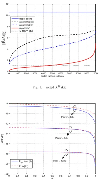
. The performance of the different randomization schemes is shown in Figure 1 where the sorted values of ˜xHA˜x are plotted, together with the upper bound, Tr[AX⋆], for different
approximation methods. The five performance curves corre-spond to different methods we described in Section II to derive the approximated solution to (4). The ones labeled ”upper bound” and ”˜x from (6)” are obtained by solving (6).The three remaining curves are the sorted maximum mismatches given by the schemes described in Algorithm 1 and versions(i)
and(ii)of Algorithm 2.10000different random vectors were used for each scheme. It can be seen that the upper bound obtained from the semidefinite relaxation is not tight. Other experiments (not shown here) indicate that the relaxation is tight in the case of 2×2channels, even though the resulting X matrix is not rank 1. Comparing the three randomization schemes, Algorithm 2, version (ii) provides the best, i.e. the combination of semidefinite relaxation, randomization and the optimization scheme in [12]. On the other hand, the more direct randomization scheme of Algorithm 1 is clearly inferior and would require a significantly larger number of randomizations to obtain a point close to the optimum.
Next, we study the influence of the Kronecker model. For this purpose, we introduce a Kronecker mismatch factor0< α < 1 such that R = Rkron +αR˜max, such that α = 0 corresponds to the Kronecker model andα= 1gives a channel that is as far as possible from being Kronecker. Here, R˜max
was obtained by scheme(ii)in Algorithm 2 which resulted in the largest norm among all methods.
The temporal covariance of disturbance matrixSQis chosen
arbitrarily and for the experiments reported in Figs 2- 3, the spatial covarianceSRis selected in such a way thatUS =UR.
In addition, The matrices R andSare normalized such that Tr{R}/Tr{S} = 1, therefore, the signal to interference ratio (SIR) is equivalent to PTr{R}/Tr{S}=P.
We employ a standard sequential quadratic programming method (fmincon in Matlab) in order to find the local
minimum of the non-linear optimization problem (8). One key component in this method is the initial points which result in different local minima. For the initial guess, the
0 1000 2000 3000 4000 5000 6000 7000 8000 9000 10000 0 2 4 6 8 10 12
sorted random indexes Upper bound Algorithm 2 (ii) Algorithm 2 (i) Algorithm 1 ˜ xfrom (6) k ˜ R( ˜x ) k 2 F
Fig. 1. sorted˜xHA˜x
0 0.1 0.2 0.3 0.4 0.5 0.6 0.7 0.8 0.9 1 −22 −20 −18 −16 −14 −12 −10 −8 α MSE(dB) P opt from (8) P* in [11] Power = 0dB Power = 5dB Power = 10dB
Fig. 2. MSE as a function of Kronecker mismatch factor for different signal to interference ratios
training sequence designed in [11] is used since it is optimal at α= 0. To observe the variation of MSE at different Kronecker mismatch factors and SIR, MSE curves are plotted in Figure 2 and Figure 3. In Figure 2 the performance has been plotted in terms ofα for different SIR. Moreover the dashed curves show the performance related to the case when we pick (10) as the pilot signal at different SIRs. The closeness of two curves, solid line and dashed line, in each SIR, implies that the training sequence design in [11] which has been done according to the Kronecker model assumption, is robust with respect to this Kronecker mismatch.
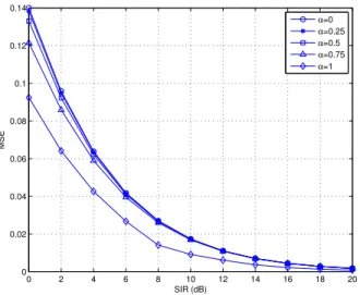
To observe the robustness of the pilot signal at high SIR region, we also plot the performance as a function of SIR at several model mismatch errors in Figure 3.
It is also interesting to investigate the effect of the interfer-ence assumptions on the performance. As mentioned in
Sec-0 2 4 6 8 10 12 14 16 18 20 0 0.02 0.04 0.06 0.08 0.1 0.12 0.14 SIR (dB) MSE α=0 α=0.25 α=0.5 α=0.75 α=1
Fig. 3. MSE as a function of SIR for different Kronecker mismatch factors
tion III, one condition which should hold in order to derive the optimal training sequence (10) isUS =UR. In order to break
this assumption, we choose the unitary matricesURandUSto
be orthogonal in the sense thatTr[UH
RUS] = 0. To find such
US, given the unitary matrix UR, we first note that UHRUS
is unitary as well. Thus, it is enough to chooseUS =URF,
whereFis a unitary matrix whose trace is equivalent to zero. One solution is to use an FFT matrix and multiply each column by a phase shift such that the diagonal elements of the re-sulting matrix is [1, ej2π/K, ej4π/K, . . . , ej2(K−1)π/K
]which provides a unitary matrixF. Figure 4 shows the performance variations for the two different interference scenarios. The SNR is set to 5dB. It can be seen that when the eigenvectors of channel and interference are orthogonal to each other, the performance loss of using (10) is slightly larger, as expected. Still the difference remains small. It should be mentioned that the diagonal eigenvalue matrix has been kept the same for both the two scenarios so that to have a fair comparison in terms of eigenvectors.
V. CONCLUSION
In this work, we have provided algorithms to determine a channel covariance matrix that is as far as possible from the Kronecker model, based on an assumption of spatial stationar-ity and the algebraic property that the covariance matrix should be positive semidefinite. The best performance is obtained using a combination of semi-definite relaxation using Schur complement for the constraint on the covariance matrix, with randomization and a second optimization procedure to find a point on the boundary of the feasible set.
These results can be used to validate the robustness of differ-ent transceiver schemes, that have been designed based on the Kronecker model. As an example of such a validation, we have illustrated the performance of optimal pilot signal design based on statistical channel information. In this particular example,
0 0.1 0.2 0.3 0.4 0.5 0.6 0.7 0.8 0.9 1 −21 −20 −19 −18 −17 −16 −15 −14 −13 −12 α MSE (dB) P* in [11], U S=UR P opt from (8), US=UR P* in [11], Tr[U R HU S]=0 P
opt from (8), Tr[UR HU
S]=0
Fig. 4. MSE as a function of Kronecker mismatch factor for different scenarios at SIR= 5dB
the numerical results indicate the the pilot design is close to optimal also if the channel is far from Kronecker.
VI. ACKNOWLEDGMENT
The authors would like to thank Efthymios Tsakonas and Dr. Joakim Jald´en for useful hints on combining the semidefinite relaxation with a Schur complement.
REFERENCES
[1] C.-N. Chuah, D. Tse, J. Kahn, and R. Valenzuela, “Capacity scaling in MIMO wireless systems under correlated fading,”IEEE Transactions on Information Theory, vol. 48, no. 3, pp. 637 –650, Mar. 2002. [2] A. Sayeed, “Deconstructing multiantenna fading channels,”IEEE
Trans-actions on Signal Processing, vol. 50, no. 10, pp. 2563 – 2579, Oct. 2002.
[3] W. Weichselberger, M. Herdin, H. ¨Ozcelik, and E. Bonek, “A stochastic MIMO channel model with joint correlation of both link ends,” IEEE Transactions on Wireless Communications, vol. 5, no. 1, pp. 90 – 100, Jan. 2006.
[4] D.-S. Shiu, G. Foschini, M. Gans, and J. Kahn, “Fading correlation and its effect on the capacity of multielement antenna systems,”IEEE Transactions on Communications, vol. 48, no. 3, pp. 502 –513, Mar. 2000.
[5] J. Kermoal, L. Schumacher, K. Pedersen, P. Mogensen, and F. Fred-eriksen, “A stochastic MIMO radio channel model with experimental validation,”IEEE Journal on Selected Areas in Communications, vol. 20, no. 6, pp. 1211 – 1226, Aug. 2002.
[6] V. Raghavan, J. Kotecha, and A. Sayeed, “Why does the kronecker model result in misleading capacity estimates?”This paper appears in: IEEE Transactions on Information Theory, vol. 56, pp. 4843 – 4864, Oct. 2010.
[7] C. Oestges, “Validity of the kronecker model for MIMO correlated channels,”IEEE 63rd Vehicular Technology Conference, vol. 6, pp. 2818 –2822, May 2006.
[8] C. Oestges, B. Clerckx, D. Vanhoenacker-Janvier, and A. Paulraj, “Impact of fading correlations on MIMO communication systems in geometry-based statistical channel models,”IEEE Transactions on Wire-less Communications, vol. 4, no. 3, pp. 1112 – 1120, May 2005. [9] E. Visotsky and U. Madhow, “Space-time transmit precoding with
imperfect feedback,”IEEE Transactions on Information Theory, vol. 47, no. 6, pp. 2632 –2639, Sep. 2001.
[10] M. Vu and A. Paulraj, “Optimal linear precoders for MIMO wireless correlated channels with nonzero mean in space-time coded systems,” IEEE Transactions on Signal Processing, vol. 54, no. 6, pp. 2318 – 2332, Jun. 2006.
[11] E. Bj¨ornson and B. Ottersten, “A framework for training-based es-timation in arbitrarily correlated rician MIMO channels with rician disturbance,”IEEE Transactions on Signal Processing, vol. 58, no. 3, pp. 1807 –1820, Mar. 2010.
[12] K. Yu, M. Bengtsson, and B. Ottersten, “On the error of kronecker structure based MIMO channel model,”Proceedings of Nordic Radio Symposium, 2004.
[13] Y. Liu, T. Wong, and W. Hager, “Training signal design for estimation of correlated MIMO channels with colored interference,”IEEE Trans-actions on Signal Processing, vol. 55, no. 4, pp. 1486–1497, Apr. 2007. [14] J. Kotecha and A. Sayeed, “Transmit signal design for optimal estimation of correlated MIMO channels,”IEEE Transactions on Signal Processing, vol. 52, no. 2, pp. 546–557, Feb. 2004.
[15] Z. Luo, W.-K. Ma, A.-C. So, Y. Ye, and S. Zhang, “Semidefinite relaxation of quadratic optimization problems,”IEEE Signal Processing Magazine, vol. 27, no. 3, pp. 20 –34, May 2010.
[16] M. Grant and S. Boyd, “CVX: Matlab software for disciplined convex programming, version 1.21,” http://cvxr.com/cvx, Oct. 2010.
[17] S. Kay, Fundamentals of Statistical Signal Processing: Estimation Theory. Englewood Cliffs, NJ: Prentice Hall, 1993.
[18] S. Loyka, “Channel capacity of MIMO architecture using the exponential correlation matrix,”IEEE Communications Letters, vol. 5, no. 9, pp. 369 –371, Sep. 2001.