ISDC
ISDC
JEM-X Analysis User Manual
April 2014 10.1 ISDC/OSA-UM-JEMX
INTEGRAL
Science Data Centre
JEM-X Analysis User Manual
Reference : ISDC/OSA-UM-JEMX
Issue : 10.1
Date : April 2014
INTEGRALScience Data Centre Chemin d’ ´Ecogia 16
CH–1290 Versoix Switzerland
Authors and Approvals
ISDC
ISDC
JEM-X Analysis User Manual
April 2014 10.1 Prepared by : M. Chernyakova P. Kretschmar JEM-X team A. Neronov V. Beckmann L. Pavan Agreed by : C. Ferrigno . . . . Approved by : T. J.-L. Courvoisier . . . .
Document Status Sheet
ISDC
ISDC JEM-X Analysis User Manual
2 April 2003 1.0 First Release.
19 May 2003 1.1 Update of the First Release.
Section 5, 9, Tables 60, 14, 21 and bibliography were up-dated.
18 July 2003 2.0 Second Release.
Sections 5, 6, 9, 8.1, Appendix C and bibliography were updated. Section8.11was added.
8 December 2003 3.0 Third Release.
Part I and the bibliography were updated. Section 6 was rewritten.
19 July 2004 4.0 Fourth Release.
Sections6,9, and the bibliography were updated. 6 December 2004 4.2 Update of Fourth Release.
Sections 6, 8.6, 9, Table 41 and the bibliography were up-dated.
3 June 2005 5.0 Fifth Release
Descriptions of j ima iros and j ima mosaic are the main changes.
21 December 2006 6.0 Sixth Release
Significant changes in the COR level, spectral extraction from mosaic images added
06 February 2007 6.0.1 Update of the Sixth Release
RMF Calibration instances updated, a new known issue added.
14 September 2007
7.0 Seventh Release: j ima iros updates, new tool j ima src locator.
25 February 2008 7.0 minor corrections.
31 August 2009 8.0 Significant changes in sections 7.6, 7.7.
26 April 2010 9.0 Several fixes in the cook book. Correction of Table 5 in Section 7.6.1 Update of known limitations and URLs 12 July 2010 9.1 Update of binning parameters example in cookbook
(j rebin rmf) 03 September
2010
9.2 Remove IMA2 viewVar parameter setting in example of sec-tion 7.6.6 (Spectral extracsec-tion) of the cookbook + minor typo
26 November 2010 9.3 Update of Figure 8 : detection limit
23 May 2012 10.0 Several updates in the cook book, known limitations, and URLs. Added new sections “Useful to know” and “Useful recipes for JEM-X data analysis” (adapted from IBIS UM). j ima mosaic updates.
8 April 2014 10.1 Updates in the cook book and clean up of known issues. 03 SEP 2014 Printed
Contents
Acronyms and Abbreviations . . . xi
Glossary of Terms . . . xii
Introduction. . . 1
I
Instrument Definition
2
1 Scientific Performance Summary . . . 22 Instrument Description. . . 3
2.1 The Overall Design . . . 3
2.2 The Detector . . . 3
2.3 Coded Mask . . . 4
3 Instrument Operations . . . 7
3.1 Telemetry Formats and Data Compression. . . 7
3.2 Energy Binning . . . 7
3.2.1 PHA Binning . . . 7
3.2.2 PI Binning . . . 8
4 Performance of the Instrument . . . 10
4.1 Position Resolution. . . 10 4.2 Energy Resolution . . . 11 4.3 Background . . . 11 4.4 Sensitivity. . . 12
II
Data Analysis
13
5 Overview . . . 136 Cookbook for JEM-X analysis . . . 16
6.1 Setting Up the Analysis Data . . . 16
6.2 Downloading Your Data . . . 17
6.3 Setting the environment . . . 18
6.4 Useful to know! . . . 19
6.5 A Walk Through the JEM-X Analysis . . . 20
6.6 Examples of Image Creation. . . 20
6.6.1 Results from the Image Step . . . 22
6.6.3 PIF-cleaning of images around strong sources. . . 24
6.6.4 The Mosaic Image . . . 24
6.6.5 Combining JEMX-1 and JEMX-2 mosaic images . . . 28
6.6.6 Finding Sources in the Mosaic Image . . . 28
6.6.7 Making images in arbitrary energy bands . . . 30
6.7 Source Spectra Extraction . . . 30
6.7.1 Spectral Extraction at SPE level . . . 30
6.7.2 Energy binning definition . . . 30
6.7.3 Spectral response generation . . . 31
6.7.4 Individual Science Windows Spectra . . . 31
6.7.5 Combining Spectra of different Science Windows . . . 33
6.7.6 Extracting Spectra from a given Position in the Sky . . . 33
6.7.7 Spectral Extraction from Mosaic Images. . . 35
6.8 Source Lightcurve Extraction . . . 37
6.8.1 Lightcurve extraction at LCR level . . . 37
6.8.2 Individual Science Windows Lightcurves . . . 37
6.8.3 Combining Lightcurves from Different Science Windows . . . 37
6.8.4 Displaying the Results of the Lightcurve Extraction . . . 38
6.8.5 Lightcurve extraction from the IMA step . . . 39
7 Useful recipes for JEM-X data analysis . . . 39
7.1 User GTIs . . . 39
7.2 Usage of the predefined Bad Time Intervals . . . 40
7.3 Rerunning the Analysis . . . 40
7.3.1 Creating a second mosaic in the Observation Group . . . 41
7.4 Combining results from different observation groups . . . 41
7.4.1 Creating a mosaic from different observation groups . . . 41
7.4.2 Combining spectra and lightcurves from different observation groups. . . 42
7.5 Create your own “user catalog” . . . 43
7.6 Barycentrisation . . . 44
7.7 Timing Analysis without the Deconvolution . . . 44
8 Basic Data Reduction . . . 47
8.1 j correction . . . 47
8.1.2 j cor position . . . 50
8.2 j gti . . . 50
8.2.1 gti create . . . 50
8.2.2 gti attitude . . . 51
8.2.3 gti data gaps . . . 51
8.2.4 gti import. . . 51
8.2.5 gti merge . . . 52
8.3 j dead time . . . 52
8.3.1 j dead time calc . . . 52
8.4 j cat extract . . . 53 8.5 j image bin . . . 53 8.5.1 j ima shadowgram . . . 54 8.6 j imaging . . . 55 8.6.1 j ima iros . . . 57 8.6.2 q identify srcs . . . 58 8.7 j src extract spectra. . . 60 8.7.1 j reform spectra . . . 60 8.8 j src extract lc . . . 60 8.8.1 j src lc . . . 60 8.9 j bin spectra. . . 61
8.9.1 j bin evts spectra . . . 61
8.9.2 j bin spec spectra . . . 62
8.9.3 j bin bkg spectra . . . 62
8.10 j bin lc. . . 62
8.10.1 j bin evts lc . . . 63
8.10.2 j bin rate lc. . . 63
8.10.3 j bin bkg lc . . . 64
8.11 Observation group level analysis . . . 64
8.11.1 j ima mosaic . . . 64
8.11.2 src collect . . . 66
8.11.3 j ima src locator . . . 66
9 Known Issues and Limitations . . . 70
A.1 Raw Data . . . 72
A.1.1 Full Imaging mode. . . 72
A.1.2 Restricted Imaging mode. . . 73
A.1.3 Spectral/Timing mode . . . 73
A.1.4 Timing mode. . . 73
A.1.5 Spectral mode . . . 74
A.1.6 Prepared Data . . . 74
A.1.7 Revolution File Data . . . 74
B Instrument Characteristics Data used in Scientific Analysis . . . 74
B.1 The IMOD group. . . 74
B.2 The BPL group. . . 76
B.3 Energy Binning: ADC to PI . . . 77
B.4 Detector positions . . . 81
B.5 Detector Response Matrix . . . 81
C Science Data Products . . . 82
C.1 j correction . . . 82 C.1.1 j cor gain . . . 82 C.1.2 j cor position . . . 82 C.2 j gti . . . 83 C.3 j dead time . . . 83 C.4 j cat extract . . . 84 C.5 j image bin . . . 84 C.6 j imaging . . . 84 C.6.1 j ima iros . . . 84 C.6.2 q identify srcs . . . 85 C.7 j src extract spectra. . . 85 C.8 j src extract lc . . . 86 C.8.1 j src lc . . . 87 C.9 j bin spectra. . . 87
C.9.1 j bin evts spectra . . . 87
C.9.2 j bin bkg spectra . . . 87
C.10 j bin lc. . . 88
C.11.1 j ima mosaic . . . 89
C.11.2 src collect . . . 89
List of Figures
1 JEM-X effective area with the mask taken into account. . . 3
2 Overall design of JEM-X and functional diagram of one unit. . . 4
3 Off axis response of JEM-X below 50 keV. . . 5
4 Collimator layout. . . 5
5 JEM-X coded mask pattern.. . . 6
6 The position resolution in the detector as a function of energy. . . 10
7 Empty field background spectrum . . . 11
8 Predicted 3σsource detection limit . . . 12
9 Decomposition of thejemx science analysisscript. . . 14
10 GUI . . . 21
11 jmx2 sky ima.fitsfile . . . 22
12 Single ScW image. . . 23
13 PIF-cleaned image . . . 25
14 jmx2 obs res.fitsfile . . . 26
15 Mosaic image . . . 27
16 Mosaic image in AIToff-Hammer projection . . . 28
17 jmx2 src loc.fitsfile . . . 29
18 Crab spectrum . . . 32
19 Spectrum of 4U 1722-30 . . . 34
20 Spectrum of 4U 1722-30 from mosaic . . . 36
21 Crab lightcurve, first energy band. . . 38
22 Detailed decomposition of thejemx science analysisscript . . . 48
23 A shadowgram with a strong on-axis source . . . 54
24 The distribution of values in an RSTI image. . . 59
25 Simplified version of the vignetting array. . . 61
List of Tables
1 JEM-X parameters and performance. . . 2
2 Characteristics of the JEM-X Telemetry Packet Formats. . . 7
3 Energy boundaries of the PI channels . . . 8
4 Overview of the JEM-X Scientific Analysis Levels. . . 13
5 Standard energy binning. . . 31
6 JEM-X imod files instance number.. . . 46
7 j cor gainparameters included into the main script. . . 49
8 gti createparameters included into the main script. . . 51
9 gti attitudeparameters included into the main script. . . 51
10 gti data gapsparameters included into the main script. . . 51
11 gti importparameters included into the main script. . . 51
12 gti mergeparameters included into the main script. . . 52
13 j cat extractparameters included into the main script . . . 53
14 j image binparameters included into the main script . . . 54
15 Parameters specific to the IMA level. . . 55
16 q identify srcsparameters included into the main script . . . 59
17 j src lcparameters included into the main script . . . 60
18 j bin evts spectraspecific to the BIN S level. . . 61
19 j bin evts spectraspecific to the BIN S level. . . 62
20 j bin bkg spectraspecific to the BIN S level . . . 62
21 j bin evts lcspecific to the BIN T level . . . 63
22 j bin rate lcparameters specific to the BIN T level. . . 63
23 j ima mosaicparameters . . . 65
24 src collectparameters specific to the IMA2 level . . . 66
25 j ima src locatorparameters . . . 67
26 List of JEM–X RAW, PRP and COR Data Structures . . . 72
27 Content ofJMXi-FULL-RAWData Structure. . . 73
28 Content ofJMXi-REST-RAWData Structure. . . 73
29 Content ofJMXi-RATE-RAWData Structure. . . 73
30 Content ofJMXi-SPTI-RAWData Structure. . . 73
31 Content ofJMXi-TIME-RAWData Structure. . . 73
33 Content ofJMXi-IMOD-GRP Group. . . 74
34 Content ofJMXi-BPL.-GRP Group. . . 76
35 Content ofJMXi-***B-ModData Structures.. . . 77
36 Content ofJMXi-GAIN-CAL-IDXIndex. . . 79
37 Content ofJMXi-GAIN-CALIndex.. . . 80
38 Content ofJEMXi-*BDS-MODData Structures. . . 80
39 Content ofJMXi-RMF.-RSP Data Structure. . . 81
40 Content ofJMXi-AXIS.-ARF Data Structure. . . 81
41 Possible corrected event STATUS values . . . 82
42 Content ofJMXi-****-CORData Structures.. . . 83
43 Content ofJMXi-GNRL-GTIData Structure. . . 83
44 Content ofJMXi-DEAD-SCPData Structure. . . 84
45 Content ofJMXi-SCAL-BKGandJMXi-SCAL-DBGData Structures. . . 84
46 Content ofJMXi-EVTS-SHD-IDX . . . 84
47 Content ofJMXi-SRCL-RESData Structure. . . 84
48 Content ofJMXi-SRCL-BSPData Structure. . . 86
49 Content ofJMXi-SRCL-SPEData Structure. . . 86
50 Content ofJMXi-SRCL-ARFData Structure. . . 86
51 Content ofJMXi-SRC.-LCRData Structure. . . 87
52 Content ofJMXi-FULL-DSP,JMXi-REST-DSPandJMXi-SPTI-DSPData Structures. . . 87
53 List of thej bin bkg spectraoutput Data Structures . . . 88
54 Content ofJMXi-DETE-LCR-IDX Data Structure. . . 88
55 Content ofJMXi-DETE-LCR Data Structure. . . 88
56 Content ofJMXi-DETE-FLC-IDX Data Structure. . . 88
57 Content ofJMXi-DETE-FLC-IDX Data Structure. . . 88
58 Content ofJMXi-MOSA-IMA-IDX . . . 89
59 Content ofJMXi-OBS.-RESData Structure. . . 89
Acronyms and Abbreviations
ADC Analog to Digital Converter
CR Cosmic Rays
DFEE Digital Front End Electronics
DPE Data Processing Electronics
DSRI Danish Space Research Institute
DXB Diffuse X-ray Background
FRSS Fixed Radiation Source System
FCFOV Fully Coded Field of View
FOV Field of View
FULL Full Imaging Format
GTI Good Time Interval
IC Instrument Characteristics
IJD Integral Julian Day
ISOC Integral Science Operations Centre
ISDC Integral Science Data Center
ISSW Instrument Specific Software
JEM-X Joint European Monitor for X-rays
HURA Hexagonal Uniformly Redundant Array
IROS Iterative Removal of Sources
MSP Microstrip Plate
OBT On Board Time
OCL Off-line Calibration
OG Observation Group
PCFOV Partially Coded Field of View
PHA Pulse Height Amplitude
PI Pulse Invariant
RATE Countrate Format
REST Restricted Imaging Format
S/C Spacecraft
SPTI Spectral-Timing Format
SPEC Spectral Format
SDAST Science Data Analysis Team
TBW To be written
TIME Timing Format
TM Telemetry
ZRFOV Zero Response Field of View
SPAG Spatial gain variation (of the microstrip plate)
Glossary of Terms
• ISDC system: the complete ground software system devoted to the processing of theINTEGRALdata and running at the ISDC. It includes contributions from the ISDC and from theINTEGRALinstrument teams.
• Science Window (ScW): For the operations, ISDC defines atomic bits of INTEGRAL operations as either a pointing or a slew, and calls them ScWs. A set of data produced during a ScW is a basic piece ofINTEGRALdata in the ISDC system.
• Observation: Any group of ScW used in the data analysis. The observation defined from ISOC in relation with the proposal is only one example of possible ISDC observations. Other combinations of Science Windows,i.e.,of observations, are used for example for the Quick-Look Analysis, or for Off-Line Scientific Analysis.
• Pointing: Period during which the spacecraft axis pointing direction remains stable. Because of the INTEGRALdithering strategy, the nominal pointing duration is of order of 20 minutes.
• Slew: Period during which the spacecraft is manoeuvred from one stable position to another, i.e., from one pointing to another.
• Shadowgram: The pattern of detected events on the microstrip plate produced when particles and xrays pass through the coded mask and hit the plate
• Sky image: Image of the sky above the telescope produced when a shadowgram integrated over a given period of time is deconvolved by the image construction software
• Mosaic: A sky image produced by merging two or more separate sky images so as to cover a greater area of sky, or to enhance the signal from a particular area of the sky.
Introduction
This document, ’JEM-X Analysis User Manual’, has been written to help you with the JEM-X specific part of theINTEGRALData Analysis.
You will find some text in blue along this manual: it is used to notify a difference with respect to the previous version of this document, or the introduction of a new section (in this case only the title is marked in blue). A more general overview on theINTEGRALData Analysis can be found in the ’Introduction to the INTE-GRALData Analysis’ [1]. For the JEM-X analysis scientific validation report see [3]
The ’JEM-X Analysis User Manual’ is divided into two major parts:
• Description of the Instrument
This part, based to some extent on the JEM-X User Manual [2], introduces theINTEGRALon-board X-Ray Monitor (JEM-X).
• Description of the Data Analysis
This part starts with an overview describing the different steps of the analysis. Then, in the Cookbook Section, several examples of analysis and their results and the description of the parameters are given. Finally, the used algorithms are described. A list of the known limitations of the current release is also provided.
In the Appendix of this document you find the description of the Raw and Prepared Data and also the description of the Scientific Products.
Part I
Instrument Definition
1
Scientific Performance Summary
The Joint European Monitor for X-rays (JEM-X) on-boardINTEGRALfulfills three roles:
• It provides complementary data at lower energies for the studies of the gamma-ray sources observed by the two main instruments, IBIS and SPI. Flux changes or spectral variability at the lower energies may provide important elements for the interpretation of the gamma-ray data. In addition, JEM-X has a higher spatial resolution than the gamma-ray instruments. This aids with the identification of sources in crowded fields.
• During the recurrent scans along the galactic plane JEM-X provides rapid alerts for the emergence of new transients or unusual activity in known sources. These sources may be unobservable by the other instruments onINTEGRAL.
• Finally, JEM-X may deliver independent scientific results concerning sources with soft spectra, serendip-itously detected in the field of view (FOV) during the normal observations.
JEM-X operates simultaneously with the main gamma-ray instruments IBIS and SPI. It is based on the same principle as the two gamma-ray instruments on INTEGRAL : sky imaging using a coded aperture mask. The performance of JEM-X is summarized in Table1.
Table 1: JEM-X parameters and performance.
Energy range 3 – 35 keV
Energy resolution† ∆E/E = 0.40×[(1/EkeV) + (1/120 keV)]1/2 Field of view (diameter)† 4.8◦ Fully illuminated
7.5◦ Half response 13.2◦ Zero response Angular resolution (FWHM) 30
Relative point source location error 10 (90% confidence radius for a 5σisolated source) Continuum sensitivity 1.2×10⁻⁴ ph cm−2s−1keV−1 @ 6 keV
for a single JEM-X unit 1.0×10⁻⁴ ph cm−2s−1keV−1 @ 30 keV
(isolated source on-axis) for a 3σ cont. detection in 105s, ∆E = 0.5E
Narrow-line sensitivity 1.6×10⁻⁴ ph cm−2s−1 @ 6 keV
(isolated source on-axis) 1.3×10⁻⁴ ph cm−2s−1 @ 20 keV for a 3σline detection in 105s Timing resolution 122µs (relative timing)
∼1 ms (absolute timing)
†The energy resolution is slowly changing (degrading) over time.
Figure 1:
JEM-X effective area with the mask taken into account. The dashed line shows the effective area before the high voltage reduction and the full curve shows efficiency when taking into account the effect of the electronic low-signal cutoff (approximately).
2
Instrument Description
2.1
The Overall Design
JEM-X consists of two identical coded-aperture mask telescopes co-aligned with the other instruments on INTEGRAL . The photon detection system consists of high-pressure imaging Microstrip Gas Chambers (MSGC) located at a distance of 3.4 m from each coded mask. Figure 2shows a schematic diagram of one JEM-X unit. A single JEM-X unit comprises 3 major subsystems: the detector, the associated electronics and the coded mask.
The two JEM-X units have been used alternatively in the past, and are currently operated simultaneously. The decision to use only one instrument at a time was made about three months after launch when a gradual loss in sensitivity had been observed in both JEM-X units, due to the erosion of the microstrip anodes inside the detector. By lowering the operating voltage, and thereby the gain of the detectors, the anode damage rate has now been reduced to a level where the survival time of the detectors seems to be assured for a further five year period. Only 6 anodes have been lost on JEM-X1 in all of 2006. Another 7 anode strips have been lost on JEM-X1 in the first 8 months of 2007. For the complete, updated list of dead anodes see http://outer.space.dtu.dk/users/oxborrow/sdast/InstrConfig/JC.BadAnodes.txt
2.2
The Detector
Each JEM-X detector is a microstrip gas chamber with a sensitive geometric area of 500 cm2 per unit. The gas inside the steel pan-shaped detector vessel is a mixture of xenon (90%) and methane (10%) at 1.5 bar pressure. The incoming photons are absorbed in the xenon gas by photo-electric absorption and the resulting ionization cloud is then amplified in an avalanche of ionizations by the strong electric field near the microstrip anodes. Significant electric charge is picked up on the strip as an electric impulse. The position of the electron avalanche in the direction perpendicular to the strip pattern is measured from the centroid of the avalanche charge. The orthogonal coordinate of an event is obtained from a set of electrodes deposited
Figure 2:
Left:Overall design of JEM-X, showing the two units, with only one of the two coded masks. Right: functional diagram of one unit.
on the rear surface of the microstrip plate (MSP).
The X-ray window of the detector is composed of a thin (250µm) beryllium foil which is impermeable to the detector gas but allows a good transmission of low-energy X-rays (see dashed curve in Fig. 1). the Be window imposes an absolute lower limit of'3 keV on the energy of X-rays coming into the detector, and hence it is meaningless to try to push the data analysis below this limit.
A collimator structure with square-shaped cells is placed on top of the detector entrance window. It gives support to the window against the internal pressure and, at the same time, limits and defines the field of view of the detector. The collimator is important for reducing the count rate caused by the cosmic diffuse X-ray background. However, the presence of the collimator also means that sources near the edge of the field of view are attenuated with respect to on-axis sources (see Fig.3). The materials for the collimator (molybdenum, copper, aluminium) have been selected in order to minimize the detector background caused by K fluorescence. Four radioactive sources are embedded in each detector collimator in order to calibrate the energy response of the JEM-X detectors in orbit. For JEM-X1 two 55Fe and two 109Cd sources were
used. For JEM-X2 all four radioactive sources are109Cd. Each source illuminates a well defined spot on the
microstrip plate. 109Cd emits 22 keV and 88 keV photons. 55Fe produces one unresolved doublet at 6 keV.
The gain of the detector gas is monitored continuously with the help of these sources. Figure4 shows the collimator layout and the locations of the calibration sources. There is one calibration source for each anode segment on the MSP. The 29.6 keV photons produced by Xe fluorescence can be detected all over the MSP and are used for offline monitoring of the gain correction by the software, and also to produce instrument model tables of the spatial gain (SPAG) variation across the detector plate. For the complete archive of these offline analyses see: http://outer.space.dtu.dk/users/oxborrow/sdast/GAINresults.html.
2.3
Coded Mask
The mask is based on a Hexagonal Uniformly Redundant Array (HURA). For JEM-X a pattern composed of 22501 elements with only 25% open area has been chosen. The 25% transparency mask actually achieves
Figure 3:
Off axis response of JEM-X below 50 keV where the collimator walls are opaque. The thick line shows the average transmission through the collimator considering all azimuth angles. The square pattern of the collimator introduces an azimuthal dependence of the throughput with a minimum and a maximum as indicated by the two thin curves (no response at ZRFOV indicated by dash-dot line).
Figure 4:
Collimator layout. In this diagram the 4 calibration sources are situated on the upper side. The dimensions are in mm, i.e. collimator length = 57 mm, radius = 130 mm
Figure 5:
Illustration of the JEM-X coded mask pattern layout without the mechanical interface. The diameter of the coded mask is 535 mm. The mask has a transparency of 25%.
better sensitivity than a 50% mask, particularly in complex fields with many sources, or in fields where weak sources should be studied in the presence of a strong source. A mask with lower transparency also has the advantage of reducing the number of events to be transmitted, while at the same time increasing the information content of the remaining events. Considering the telemetry allocation to JEM-X, this means an improved overall performance for the instrument, particularly for observations in the plane of the Galaxy. The mask height above the detector ( 3.4 m) and the mask element dimension (3.3 mm) define together the angular resolution of the instrument, in this case 3’. Figure5illustrates the JEM-X coded mask pattern.
3
Instrument Operations
3.1
Telemetry Formats and Data Compression
JEM-X data can be transmitted in several different telemetry formats which vary in their information content for position, energy or time and the required bandwidth per event. In addition, a “grey filter” mechanism exists eliminating a fraction of the incoming events in a randomized way. The possible transmission settings range from 32/32 to 1/32 of the incoming events. These mechanisms allow the instrument to cope with sources of very different brightness despite its limited telemetry allocation.
For formats with poor time resolution (REST, SPEC) countrate data packets are also transmitted to provide some data for timing analysis. However countrate data is not an independent data format.
For a given observation a primary and a secondary telemetry format are defined and they can be identical. If the observed data rate is too high to be transmitted completely, first the grey filtering will be increased to reduce the number of processed events. Should this not be sufficient the instrument will autonomously switch to the secondary telemetry format, continuing to adapt the grey filter as necessary. For decreasing input rates the instrument will reduce the filtering and possibly switch back to the primary format. All these changes are driven by the filling status of an on-board buffer, the mechanism includes a certain hysteresis in order to avoid rapid switching between formats.
The characteristics of primary and secondary telemetry formats are listed in Table2. The default primary format is Full Imaging and the default secondary format is Restricted Imaging. Note that in the Spectral Timing format the actual spectral resolution will be slightly lower than that of the Full Imaging mode due to spatial gain variations in the detector. It is recommended, however, that the full imaging format is used both as primary and secondary format.
Table 2: Characteristics of the JEM-X Telemetry Packet Formats.
Detector Image Timing Spectral Events
Format Name Resolution Resolution Resolution per
(pixels) (channels) packet
Full Imaging (FULL) 256 x 256 1/8192s = 122µs 256 ≤105 Restricted Imaging (REST) 256 x 256 ≤32 s 8 ≤320
Countrate ( ) None 1/8 s = 125 ms 1 n/a
Spectral Timing (SPTI) None 1/8192s = 122µs 256 ≤210
Timing (TIME) None 1/8192s = 122µs None ≤550
Spectrum (SPEC) None 1/8s = 125 ms 64 n/a
3.2
Energy Binning
3.2.1 PHA BinningThe energy values of the events provided in the telemetry are given as a bin number from 0 to 255. These are non-linear groupings of the original 4096 bins of the on-board Analog to Digital Converter (ADC). While the ADC channels are highly linear, the PHA bins are designed to be logarithmic so that the energy resolution of the bins parallels that of the detector. The actual grouping of the ADC channels into PHA telemetry bins is determined by a lookup table used by the Data Processing Electronics (DPE) to pack the telemetry. After the high voltage reductions this table has been updated to match the changed ADC signal strengths. See also AppendixB.3for more details.
3.2.2 PI Binning
The PI bin limits in keV have been defined so that the entire energy range (nominally 3–100 keV) is covered and the binsize is a more or less constant fraction of the detector resolution. The PI binning table for the Full Imaging mode with the highest number of bins (256) is shown in Table3. See Appendix B.3for more details.
Table 3: Energy boundaries of the PI channels
PI Emin Emax PI Emin Emax PI Emin Emax
0 0.00 0.06 86 6.24 6.32 171 17.90 18.16 1 0.06 0.12 87 6.32 6.40 172 18.16 18.42 2 0.12 0.18 88 6.40 6.48 173 18.42 18.68 3 0.18 0.24 89 6.48 6.56 174 18.68 18.94 4 0.24 0.30 90 6.56 6.64 175 18.94 19.20 5 0.30 0.36 91 6.64 6.72 176 19.20 19.46 6 0.36 0.42 92 6.72 6.80 177 19.46 19.72 7 0.42 0.48 93 6.80 6.88 178 19.72 19.98 8 0.48 0.54 94 6.88 6.96 179 19.98 20.24 9 0.54 0.60 95 6.96 7.04 180 20.24 20.50 10 0.60 0.66 96 7.04 7.12 181 20.50 20.76 11 0.66 0.72 97 7.12 7.20 182 20.76 21.02 12 0.72 0.78 98 7.20 7.28 183 21.02 21.28 13 0.78 0.84 99 7.28 7.36 184 21.28 21.54 14 0.84 0.90 100 7.36 7.44 185 21.54 21.80 15 0.90 0.96 101 7.44 7.52 186 21.80 22.06 16 0.96 1.02 102 7.52 7.60 187 22.06 22.32 17 1.02 1.08 103 7.60 7.68 188 22.32 22.58 18 1.08 1.14 104 7.68 7.76 189 22.58 22.84 19 1.14 1.20 105 7.76 7.84 190 22.84 23.10 20 1.20 1.26 106 7.84 7.92 191 23.10 23.36 21 1.26 1.32 107 7.92 8.00 192 23.36 23.72 22 1.32 1.38 108 8.00 8.08 193 23.72 24.08 23 1.38 1.44 109 8.08 8.16 194 24.08 24.44 24 1.44 1.50 110 8.16 8.24 195 24.44 24.80 25 1.50 1.56 111 8.24 8.32 196 24.80 25.16 26 1.56 1.62 112 8.32 8.42 197 25.16 25.52 27 1.62 1.68 113 8.42 8.52 198 25.52 25.88 28 1.68 1.74 114 8.52 8.62 199 25.88 26.24 29 1.74 1.80 115 8.62 8.72 200 26.24 26.60 30 1.80 1.86 116 8.72 8.82 201 26.60 26.96 31 1.86 1.92 117 8.82 8.92 202 26.96 27.32 32 1.92 2.00 118 8.92 9.02 203 27.32 27.68 33 2.00 2.08 119 9.02 9.12 204 27.68 28.04 34 2.08 2.16 120 9.12 9.22 205 28.04 28.40 35 2.16 2.24 121 9.22 9.32 206 28.40 28.76 36 2.24 2.32 122 9.32 9.42 207 28.76 29.12 37 2.32 2.40 123 9.42 9.52 208 29.12 29.48 38 2.40 2.48 124 9.52 9.62 209 29.48 29.84 39 2.48 2.56 125 9.62 9.72 210 29.84 30.20 40 2.56 2.64 126 9.72 9.82 211 30.20 30.56 41 2.64 2.72 127 9.82 9.92 212 30.56 30.92 42 2.72 2.80 128 9.92 10.08 213 30.92 31.28 43 2.80 2.88 129 10.08 10.24 214 31.28 31.64 44 2.88 2.96 130 10.24 10.40 215 31.64 32.00 45 2.96 3.04 131 10.40 10.56 216 32.00 32.36 46 3.04 3.12 132 10.56 10.72 217 32.36 32.72
47 3.12 3.20 133 10.72 10.88 218 32.72 33.08 48 3.20 3.28 134 10.88 11.04 219 33.08 33.44 49 3.28 3.36 135 11.04 11.20 220 33.44 33.80 50 3.36 3.44 136 11.20 11.36 221 33.80 34.16 51 3.44 3.52 137 11.36 11.52 222 34.16 34.52 52 3.52 3.60 138 11.52 11.68 223 34.52 34.88 53 3.60 3.68 139 11.68 11.84 224 34.88 36.16 54 3.68 3.76 140 11.84 12.00 225 36.16 37.44 55 3.76 3.84 141 12.00 12.16 226 37.44 38.72 56 3.84 3.92 142 12.16 12.32 227 38.72 40.00 57 3.92 4.00 143 12.32 12.48 228 40.00 41.28 58 4.00 4.08 144 12.48 12.64 229 41.28 42.56 59 4.08 4.16 145 12.64 12.80 230 42.56 43.84 60 4.16 4.24 146 12.80 12.96 231 43.84 45.12 61 4.24 4.32 147 12.96 13.12 232 45.12 46.40 62 4.32 4.40 148 13.12 13.28 233 46.40 47.68 63 4.40 4.48 149 13.28 13.44 234 47.68 48.96 64 4.48 4.56 150 13.44 13.60 235 48.96 50.24 65 4.56 4.64 151 13.60 13.76 236 50.24 51.52 66 4.64 4.72 152 13.76 13.92 237 51.52 52.80 67 4.72 4.80 153 13.92 14.08 238 52.80 54.08 68 4.80 4.88 154 14.08 14.24 239 54.08 55.36 69 4.88 4.96 155 14.24 14.40 240 55.36 56.64 70 4.96 5.04 156 14.40 14.56 241 56.64 57.92 71 5.04 5.12 157 14.56 14.72 242 57.92 59.20 72 5.12 5.20 158 14.72 14.88 243 59.20 60.48 73 5.20 5.28 159 14.88 15.04 244 60.48 61.76 74 5.28 5.36 160 15.04 15.30 245 61.76 63.04 75 5.36 5.44 161 15.30 15.56 246 63.04 64.32 76 5.44 5.52 162 15.56 15.82 247 64.32 65.60 77 5.52 5.60 163 15.82 16.08 248 65.60 66.88 78 5.60 5.68 164 16.08 16.34 249 66.88 68.16 79 5.68 5.76 165 16.34 16.60 250 68.16 69.44 80 5.76 5.84 166 16.60 16.86 251 69.44 70.72 81 5.84 5.92 167 16.86 17.12 252 70.72 72.00 82 5.92 6.00 168 17.12 17.38 253 72.00 73.28 83 6.00 6.08 169 17.38 17.64 254 73.28 74.56 84 6.08 6.16 170 17.64 17.90 255 74.56 81.92 85 6.16 6.24
The complete table can also be found in JMXi-IMOD-GRP structure, in extension JMXi-FBDS-MOD. The Xe instrumental background line which is used to verify the gain calibration of the instrument should appear in the channel 209.
4
Performance of the Instrument
The properties described in the following have been derived in part from pre-flight calibration measurements and modeling and in part from calibration observations in orbit. JEM-X has had major changes of its configuration since launch, the most important being a reduction of the high voltages reducing the gas gain from 1500 down to 500 for JEM-X 1 and to 750 for JEM-X 2. These changes also affect the instrument performance.
4.1
Position Resolution
The position determination accuracy depends on the number of source and background counts and on the position in the Field of View (FOV). Off-axis the collimator blocks some of the source photons and beyond the fully coded FOV (FCFOV) the coding is incomplete.
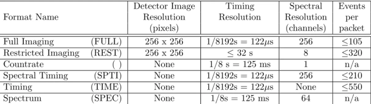
Figure6shows the position resolution for a source on axis as function of energy. The cause of the degradation below 10 keV is the signal-to-noise ratio of the front-end electronics. The energy dependence of the position resolution above 10 keV is determined by the increase of the primary photoelectron range with energy. The position resolution is slightly degraded compared to the ground calibrations.
Figure 6:
The calculated position resolution in the JEM-X 1 and JEM-X 2 detectors as a function of energy valid after 2002-11-09 (JEM-X 1) and after 2002-11-12 (JEM-X 2).
4.2
Energy Resolution
The energy resolution has been determined in the laboratory as ∆E/E(F W HM) = 0.40·p
1/E[keV] + 1/120 keV.
This value has not been significantly affected by the gain change and the corresponding slight rise in impor-tance of the electronic noise.
4.3
Background
The local radiation environment is mainly produced by two components: the diffuse X-ray background (DXB) and cosmic rays (CR). Most of the latter are rejected on-board with a combination of pulse height, pulse shape, anti-coincidence and “footprint” evaluation techniques. These techniques allow a particle rejection efficiency of>99.9% with carefully tuned selection parameters. This high rate of background rejection has ensured that there has been no significant increase in background events in the telemetry despite the steady increase in the CR rate at Solar minimum.
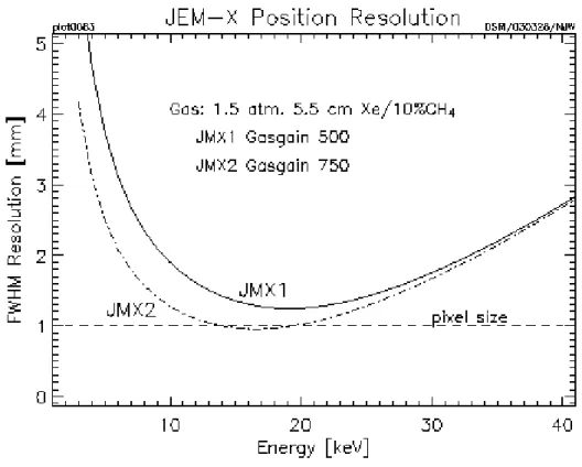
Figure7 shows an actual background spectrum which is composed of the diffuse X-ray background, instru-mental background due to the interactions with cosmic rays and three strong instruinstru-mental lines due to the cooper and molybdenum in the collimator (8.04 keV and 17.4 keV) and Xe fluorescence from the detector gas at 29.6 keV.
Figure 7:
Empty field background spectrum measured with the nominal detector gain of 1500 (left) compared to the background spectrum with the reduced gain of 500 (right). After these measurements the rejection criteria have been adjusted (2003-02-25), but no blank fields have been observed for a longer period since then. The background has increased with about 10-15% at higher energies and with 20-30% below 10 keV after the adjustment.
4.4
Sensitivity
The sensitivity achieved for source detection and flux determination also depends on the performance of the deconvolution software. Figure8shows the 3σdetection limit as a function of observation time.
The changes in gas gain and corresponding changes in signal patterns led to a large fraction of events being classified as background and rejected on-board until new selection criteria could be determined and uploaded (2003-03-25, revolution 45). Even with the new optimized selection criteria the detector sensitivity below 5 keV is reduced.
Figure 8:
Source detection capabilities in the 3 to 10 keV (resp. 10 to 25 keV) band as function of effective accumulated observation (exposure) time in JEM-X mosaic images corrected for dead time, grey filter and vignetting effects. The thick solid curve is obtained from simulations where an isolated source must be detected at 3σin the deconvolved image. The dashed line represents the case where there are additional sources in the field of view giving a background corresponding to a total of 1 Crab. Examples of actual observations are given: the source 3C 273 and the other empty circles are instances of isolated sources, while the crossed circles represent sources observed in the crowded Galactic Centre region. Theσ-values given in parentheses are obtained from a measure of the highest source pixel in significance mosaic maps with default pixel size (1.5 arcmin).
Part II
Data Analysis
5
Overview
The scientific analysis performed by the user on the data collected by the three high-energy instruments on-boardINTEGRALhas a lot of commonality, despite the various differences in detail. In a certain step, for example, events are corrected for instrumental fingerprints, in another one events are binned into detector maps, and in yet another step sky images are derived by image deconvolution.
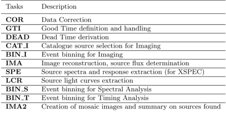
In order to make this more transparent for scientists working with data from several instruments, so-called Analysis Levels were identified by the ISDC and designated with unique labels. The order of these levels, the detailed processing and the details of the outputs may differ across instruments, but in general, a given level will mean similar tasks and similar outputs for JEM-X, IBIS, and SPI. The list of all levels is given in the Introduction to theINTEGRALData Analysis [1]. For JEM-X the following levels have been defined:
Table 4: Overview of the JEM-X Scientific Analysis Levels.
Tasks Description
COR Data Correction
GTI Good Time definition and handling
DEAD Dead Time derivation
CAT I Catalogue source selection for Imaging
BIN I Event binning for Imaging
IMA Image reconstruction, source flux determination
SPE Source spectra and response extraction (for XSPEC)
LCR Source light curves extraction
BIN S Event binning for Spectral Analysis
BIN T Event binning for Timing Analysis
IMA2 Creation of mosaic images and summary on sources found
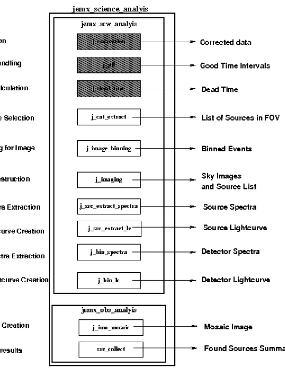
Figure9 shows the Scientific Analysis overview. The details of each step are briefly discussed below.
COR – Data Correction (j correction)
Corrects science data for instrumental fingerprints such as energy and position corrections, as well as flagging events of dubious quality. Look up tables of pre-flight corrections are used, as well as tables of in-flight calibrations determined by offline analysis of science data, calibration spectra, and instrumental background lines. Dynamic determination of known transient problems (e.g. hotspots on the detector) is also done in this level. The majority of calibration tables are stored in the Instrument Model group, JMXi-IMOD-GRP (with i = 1 and 2 for JEM-X1 and JEM-X2, respectively), but the offline gain history Instrument Characteristics tables are stored separately in JMXi-GAIN-OCL data structures. The latter are also located automatically by the OSA software just like the IMOD group. GTI – Good Time Handling (j gti)
Good Time Intervals (GTIs) are used in the analysis to select only those data taken while the detector was considered to work correctly. The corresponding data structures consist simply of a list of start and stop times of those intervals considered “good”. Usually, these intervals are generated based on the following data:
2. The satellite stability as recorded in the attitude data. 3. Gaps (lost packets) in the telemetry flow.
In addition, this step excludes by default periods when the instrument configuration is not adapted to the production of scientific works, either because of hardware problems or because of intentional modifications of the instrument configurations for the purpose of testing and calibrations. These periods are marked as ”bad time intervals”in the Instrument Characteristics data.
DEAD – Dead and Live Times (j dead time)
For each 8 second onboard polling cycle, this level calculates the dead time during which photons are lost due to finite read in time of registers, event processing time, grey filter losses, buffer losses and double event triggers.
CAT I – Catalogue Source Selection (j cat extract)
Selects a list of known sources from the given catalogue. Creates a source data structure, containing source location and expected flux values.
BIN I – Event Binning for Imaging (j image binning)
Defines the energy bins to be used for imaging, selects good events within the GTI, and creates shadowgrams. Works only on FULL and REST data (see Table2).
IMA – Image Reconstruction (j imaging)
Generates sky images and performs search for significant sources. If sources are detected, a new source data structure is created, including part of the information from the input catalogue concerning the identified sources. Works only on FULL and REST data (see Table 2)
SPE – Spectra Extraction (j src extract spectra)
Extracts spectra for individual sources found at IMA step, and produces the specific response files (ARFs) needed for spectral fitting with the XSPEC package. Works only on FULL data (see Table2). LCR – Extract Source Light Curves (j src extract lc)
Produces light curves for individual sources. Works only on FULL data (see Table2) BIN S – Event Binning for Spectral Analysis (j bin spectra)
Creates detector spectra, i.e spectra of all events recorded within the GTI are corrected for greyfilter, ontime and deadtime. A series of spectra resolved in time or phase over a given period can be produced. BIN T – Creates Detector Light Curves (j bin lc)
Creates binned lightcurves for entire detector area.
IMA2 – Mosaic Image Creation (j ima mosaic, src collect)
Generates mosaic sky images and creates the list of all found sources. Works only on FULL and REST data (see Table2)
Since October 18, 2004, all publicINTEGRALdata are available including already the correction step, and also the instrumental GTI and deadtime handling have been already performed at the science window level. This allows to speed up the scientific analysis of JEM-X data as there is no need to redo the COR, GTI and DEAD levels, but you can directly start JEM-X analysis from the CAT I level.
It is however recommended that users run the science analysis from the COR level onwards, especially after downloading new software, and IMOD/IC files. This will undoubtedly give better results than the archived data. Archived data necessarily fossilize our understanding of the instruments as it was at the time of the archival processing and can therefore be several years out of date since our knowledge of the instruments, and the software to process the data is still improving.
6
Cookbook for JEM-X analysis
The Cookbook describes how to use the OSA JEM-X software. It covers the following steps:
• Setting up the analysis data
• Setting the environment
• Launching the analysis
• Interpreting the results
We assume that you have already successfully installed the ISDC Off-line Scientific Analysis (OSA) Software version 10.1 (The directory in which OSA is installed is referred later as the ISDC ENV directory). If this is not the case, look at the “Installation Guide for the INTEGRAL Off-line Scientific Analysis” [4] for detailed help.
6.1
Setting Up the Analysis Data
In order to set up a proper environment, you first have to create an analysis directory (e.g jmx data rep) and “cd” into it:
mkdir jmx_data_rep cd jmx_data_rep
setenv REP_BASE_PROD $PWD
This working directory will be referred to as the REP BASE PROD directory in the following. All the data required in your analysis should then be available from this “top” directory, and they should be organized as follows:
• scw/ : data produced by the instruments (e.g., event tables) cut and stored by ScWs
• aux/: auxiliary data provided by the ground segment (e.g., time correlations)
• cat/ : ISDC reference catalogue
• ic/: Instrument Characteristics (IC), such as calibration data and instrument responses
• idx/: set of indices used by the software to select appropriate IC data
The JEM-X example presented below is based on observations of the Crab from Revolution 102.
Part of the required data may already be available on your system1. In that case, you can either copy these data to the relevant working directory, or better, create soft links as follows
ln -s directory_of_ic_files_installation__/ic ic ln -s directory_of_idx_files_installation__/idx idx ln -s directory_of_cat_installation__/cat cat ln -s directory_of_local_archive__/scw scw ln -s directory_of_local_archive__/aux aux
1For installation of the Instrument Characteristics files (OSA IC package) and the Reference Catalogues (OSA CAT package),
JEM-X calibration files are continuously produced by the JEM-X Team for new revolutions. To be sure to have all the latest calibrations, update your copy of the Instrument Characteristics each time you want to analyse new data, using the rsync command:
rsync -Lzrtv isdcarc.unige.ch::arc/FTP/arc_distr/ic_tree/prod/ directory_of_ic_files_installation__
This command will download the Instrument Characteristics files (icandidxdirectories) to your directory_of_ic_files_installation__.
Then, just create a file ’jmx.lst’ containing the 2 lines: scw/0102/010200210010.001/swg.fits[1]
scw/0102/010200220010.001/swg.fits[1]
which is the list of ScWs you want to analyse (technically, we call them DOLs -Data Object Locators-, i.e. a specified extension in a given FITS file). 2
This file name ‘jmx.lst’ will be used later as an argument for the og create program (see section6.5). Alternatively, if you do not have any of the above data on your local system, or if you do not have a local archive with the scw/ and the aux/ branch available, follow the next section instructions to download data from the ISDC WWW site.
6.2
Downloading Your Data
To retrieve the required analysis data from the archive, go to the following URL: http://www.isdc.unige.ch/integral/archive.
You will reach the W3Browse web page which will allow you to build a list of Science Windows (ScWs) needed to create your observation group for OSA.
• Type the name of the object (Crab) in the ‘Object Name Or Coordinates:’ field.
• Click on the ’More Options’ button at the top or at the bottom of the web page.
• Deselect the ’All’ checkbox at the top of the Catalog table, and select the ‘SCW - Science Window Data’ one.
• Press the ‘Specify Additional Parameters’ button at the bottom of the web page.
• Deselect the ‘View All’ checkbox (press twice on it) at the top of the Query table.
• Select ‘scw id’ and put the value ‘0102*’ (without the quotes) to specify all Scws from Revolution 102.
• Select ‘scw type’ and put the value ‘pointing’ (without the quotes), or simply ‘po*’ to get only pointings.
• Press the ‘Start Search’ button at the bottom of the web page. At this point, you should be at the Query Results page with all the Scws available for revolution 102.
• Sort the ‘Scw id’ column by clicking on the left arrow below the column name. You can then select the two Scws we are interested in, i.e 010200210010 and 010200220010.
Press the ‘Save SCW list for the creation of Observation Groups’ button at the bottom of that table and save the file with the name ‘jmx.lst’. The file name ‘jmx.lst’ will be used later as an argument for the og_createprogram (see section6.5). In this file, you should find the 2 lines:
2When an analysis script asks you to specify the DOL, you should specify the path of the corresponding FITS file, and the
corresponding name or number of the data structure in square brackets(do not forget that numbering starts with 0!). See more details in the Introduction to the INTEGRAL Data Analysis [1].
scw/0102/010200210010.001/swg.fits[1] scw/0102/010200220010.001/swg.fits[1]
You should then download the data pressing the ’Requestdata products for selected rows’ button. In the ‘Public Data Distribution Form’, provide your e-mail address and press the ‘Submit Request’ button. You will be e-mailed the required script to get your data and the instructions for the settings of the IC files and the reference catalogue. Just follow these instructions.
6.3
Setting the environment
Before you run any OSA software, you must also set your environment correctly.
The commands below apply to thecshfamily of shells (i.ecshandtcsh) and should be adapted for other families of shells3.
In all cases, you have to set theREP BASE PRODvariable to the location where you perform your analysis (e.g the directory jmx data rep). Thus, type:
setenv REP_BASE_PROD $PWD
Then, if not already set by default by your system administrator, you should set some environment variables and type:
setenv ISDC_ENV directory_of_OSA_sw_installation
setenv ISDC_REF_CAT $REP_BASE_PROD/cat/hec/gnrl_refr_cat_0031.fits\[1] source $ISDC_ENV/bin/isdc_init_env.csh
The idea is to:
• set ISDC ENVto the location where OSA is installed
• set ISDC REF CATto the DOL of the ISDC Reference Catalog
• run the OSA set-up script (isdc init env.csh) which initializes further environment variables relative to ISDC ENV.
Besides these mandatory settings, there are two optional environment variables (COMMONLOGFILE and COMMONSCRIPT) which are useful.
• By default, the software logs messages to the screen (STDOUT). To have also these messages in a file (i.e common log.txt) and make the output chattier4, use the command:
setenv COMMONLOGFILE +common_log.txt
• When you launch the analysis, the Graphical User Interface (GUI) is launched. As your level of expertise with the software increases, you may wish to not have the GUIs pop up when you launch your analysis. In this case, the variable COMMONSCRIPT must be defined:
setenv COMMONSCRIPT 1
3If the setenv command fails with a message like:‘setenv: command not found’ or ‘setenv: not found’, then you are probably
using the sh family. In that case, please replace the command ‘setenv my variable my value’ by the following command sequence ‘my variable=my value ; export my variable’
In the same manner, replace the command ‘source my script’ by the following command ‘. my script’ (the ‘.’ is not a typo!).
When the GUI is disabled, parameters can be specified on the command line typing ’name = value’ after the script name.
To revert and have the GUI again, unset the variable: unsetenv COMMONSCRIPT
6.4
Useful to know!
In this section we report some general information that might be useful when running OSA software. Most of these information can be found also in the IBIS Cookbook5.
• How do I get some help with the executables?
All the available help files are stored under $ISDC ENV/help. To visualize a help file interactively type tool name --honce your environment is set (i.e. the commandwhich tool name should return the path to it).
• Where are the parameter files and how can I modify them?
All the available executables for the analysis of INTEGRAL data are under $ISDC ENV/bin. The corresponding parameter files are stored under $ISDC ENV/pfiles/*.par. The first time you launch a script, the system will copy the specific tool.par from $ISDC ENV/pfiles/ to a local directory (/user name/pfiles/). The parameter file in the local directory is the one used for the analysis and is the one you can modify. If this parameter file is missing (e.g. you have deleted it), the system will just re-copy it from $ISDC ENV/pfiles/ as soon as you launch the script again. The system knows what to copy from where thanks to the $PFILES environment variable that is also used in FTOOLS (http://heasarc.gsfc.nasa.gov/ftools/). Each parameter is characterized with a letter that specifies the parameter type, i.e:
“q” (query) parameters are always asked to the user
“h” (hidden) parameters are not asked to the user and the indicated value is used
“l” (learned) parameters are updated with the user’s value during the use of the program.
The GUI is a fast and easy way to change the parameters, see also the explanation at the end of this section.
• What are groups and indices?
The ISDC software makes extensive use of groups and indices. While it is not necessary to grasp all the details of these concepts, a basic understanding is certainly quite useful.
As implied by their names, ”groups” make possible the grouping of data that are logically connected. Groups can be seen as a kind of data container, not completely unlike standard directories. At ISDC, we create separate groups for each pointing, in which we store the many different data types produced by INTEGRAL and its instruments. The user then only has to care about one file, the group, many tens of files being silently included. Several pointings (the “Science Window Groups”) can be arbitrarily grouped into bigger groups (the “Observation Group”) to select data very efficiently according to the user’s needs.
Indices are a special kind of groups, which differ only in the fact that all the the data sets they contain are similar and that the indices know the properties of the data sets they contain. Indices are a kind of poor man’s database. For example, an imaging program creates several images of different types (flux map, significance map,...) in different energy bands. These images are stored in an index, in which the image type and energy band information is replicated. ISDC software is then able to select very efficiently the needed images. The user can also make use of the indices; just by looking at the index (for instance using “fv”), the user can identify immediately the content of each image.
• Why do I need “[1]” after a FITS file name?
A FITS file can have many extensions and sometimes it is necessary to specify as input to a given pa-rameter not the file name alone (file.fits) but the extension too (file.fits[1], orfile.fits[2],
etc). The file name with a specified data structure (extension) is called DOL (Data Object Loca-tor). When you modify the parameter file itself (see above) or use the GUI, the extension will be correctly interpreted in the file.fits[1]case. On the command line though, the normal CFITSIO and FTOOLS rules apply, i.e. you have to specify it as one of the following
file.fits\[1] file.fits+1 "file.fits[1]".
Note that if no extension is specified explicitly then the first one ([1]) will be used by default.
• What are the general functionalities of the GUI?
When you launch the analysis, by default the GUI is launched, providing an opportunity to set the values of all desired parameters, see Figure 10. On the right side of the panel you see the following buttons:
– Save as– With the “Save As” - button a file is created. This file stores all parameters as they are currently defined in the GUI as a command line script. This file is an executable one and calling it from the command line will launch the instrument analysis program with the parameters as they were defined in the GUI.
– Load With the “Load” - button a previously saved file (see “Save As”) can be read and the GUI will update all parameters with the values as they are defined in the loaded file.
– Reset With the “Reset” - button the parameters in the GUI will be reset to the default values as they are defined in the parameter file of the instrument analysis program and stored in the $ISDC ENV/pfiles directory.
– RunWith “Run” - button the analysis is launched.
– Quit With “Quit” - button you quit the program without analysis launch.
– Help With “Help” - button the help file of the main script is opened in a separate window. – hidden With the “hidden” - button you have an access to the hidden parameters with values
defined by the instrumental teams. Change them with care!
The environment variableCOMMONSCRIPTis used to disable/enable the GUI (see section6.3).
6.5
A Walk Through the JEM-X Analysis
After setting up the data and the environment, you are ready to call the analysis script on the Crab region observations defined above and stored in the jmx.lst file.
Firstly, create an Observation Group (see the description of the executableog create in the “Toolbox” and “Data Analysis” sections of the Introduction to theINTEGRALData Analysis [1]):
og_create idxSwg=jmx.lst ogid=crab baseDir="./" instrument=JMX2
As a result, the directory $REP BASE PROD/obs/crab will be created6. It contains the files og jmx2.fits andswg idx jmx2.fits as well as the subdirectoryscwnecessary for the analysis. In the latest version of og create, the file indicated in idxSwg is automatically interpreted as a fits file when the name includes a “+” or “[” sign.
6.6
Examples of Image Creation
Now you can go to the directory created withog createand start the analysis
6To create the structure for both JemX units at the same time, it is possible to call og create only once, with the parameter
cd obs/crab
jemx_science_analysis startLevel="COR" endLevel="IMA" nChanBins=-4 jemxNum=2
The above command launches the analysis which will run from the Correction step (startLevel="COR") up to the image creation level (endLevel="IMA"). It is important to specify that we are interested in the second of JEM-X instruments: jemxNum=2. nChanBinsparameter specifies the energy binning (see section6.7.2for details).
At the beginning the script launches the GUI (Fig. 10) and you can check the parameter settings (the full
Figure 10: GUI for JEM-X science analysis.
list of the parameters is given in Table60). Only the most important parameters (shown in bold in Table60) appear within the main panel of GUI. To access the other “hidden” parameters click on the button “hidden” on the right side of the panel.
In the upper frame of the front panel called “General” you can choose at which level you want to start and stop the script execution. In the Overview chapter you have seen that there are different processing levels of the analysis. You can choose to run only some of them. The default settings of thejemx science analysis script are
startLevel="COR" start the script at COR level, endLevel="IMA2" stop the script at IMA2 level.
It is advisable always to start with level COR. This will allow the processing of the data using the latest knowledge of the calibration of the instrument.
If you want to skip some levels, click on the “hidden” button on the right of the GUI panel to access the whole set ofjemx science analysisparameters. In the frame “General” you find theskipLevelsparameter. However, be always careful while setting this parameter – levels often depend on the previous ones, so make sure that your selection makes sense. Another useful hidden parameterIMA skyImagesOutin theIMAsection enables you to choose the types of images which you want to output7.
7Several types of images may be produced: the vignetting-corrected intensity image, called RECONSTRUCTED, the variance
imageVARIANCE,RECTIFIED(raw intensity image),RESIDUAL(residuals left after removing all found sources) andEXPOSURE(the exposure map).
The source flux is extracted using the IMA step, in order to profit from the vast improvement in the modelling of the JEM-X instruments achieved in OSA 8. With OSA 10.1 the images are extracted by default in the same energy binning specified under ”General Binning Tasks”. To generate images in arbitrary energy bands, see section 6.6.7. As in the previous OSA versions, the optimal source detection is still obtained through j ima iros in 3 default energy ranges: 3-7 keV, 7-11 keV and 11-20 keV. The checkbox IMA detImagesOutenables you to output also the images in these pre-defined energy bands. This option is not recommended if you want to extract a spectrum from the mosaic image later.
In the middle of the GUI front panel you have a possibility to choose a “user input catalog” (the parameter CAT I usrCat). At the moment you can leave it empty (the software will use the generalINTEGRALsource catalog for the analysis). However, for the correct extraction of spectra and lightcurves of the sources it is recommended to create a “user catalog” with the positions of the sources for which you plan to extract the spectra and/or the lightcurves. We will come back to this in the following sections (and sect.7.5).
Once you are satisfied with the settings, save them by pressing the “Save As” button at the front panel of GUI and then press “Run” to start the data reduction.
6.6.1 Results from the Image Step
Afterjemx science analysisfinishes its operation, the results are stored separately for each ScW of the obser-vation group. They are located in the subdirectories namedscw/RRRRPPPPSSSF.001/(whereRRRRPPPPSSSF is the number of the ScW).
Go to one of these directories and have a look at the files cd scw/010200210010.001/
ls
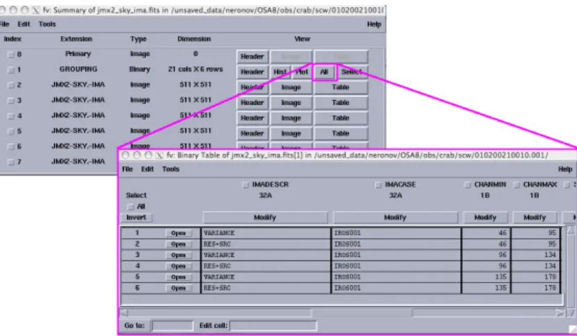
This is the output from all the processing steps done by the script. The output image isjmx2 sky ima.fits. You can check it using e.g. fv:
fv jmx2_sky_ima.fits
You will find that this file contains 7 extensions: the index of all images, 3 cleaned sky images (RECONSTRUCTED type), and 3 variance maps, one for each of the 3 selected energy bands (see Fig. 11).
Figure 11:The content ofjmx2 sky ima.fitsfile.
In the file jmx2 srcl res.fitsyou find a list of all found sources, the energy bands, and the derived flux values, and in the file jmx2 srcl cat.fits the list of the sources in the input catalog. You can see that
Figure 12:
The image of Crab region. Catalog sources in the FOV are shown with white circles. The only found source (Crab) is shown with a red box.
most of the catalog sources were not found, as they are too weak. When you run the lightcurve and spectra extraction steps the results would be produced for all sources listed injmx2 srcl res.fits.
Since OSA10 images are produced with counts per cm2. With OSA10.1 source spectra and lightcurves show
countrates per unit of detector area, in agreements with OGIP standards requirements. To extract the correct source fluxes it is fundamental to use OSA10.1 with the latest available IC files.
There is a nice way to locate the found sources as well as the catalog sources on the sky image. To do it use the utilitycat2ds9:
cat2ds9 jmx2_srcl_res.fits\[1] found.reg symbol=box color=red cat2ds9 jmx2_srcl_cat.fits\[1] cat.reg symbol=circle color=white
(to find out more about this program typecat2ds9 --hin the command line). With the help of the above two commands the two files found.reg and cat.reg are created. They contain the lists of all the found sources and all the catalog sources, respectively.
With the help ofds9viewer you can display the sky images in any of the avilable energy bands. For example, to look at the 7–11 keV image which (if you used the optionIMA detImagesOut=yes) is contained in the 5th extension of thejmx2 sky ima.fitsfile you can type
ds9 jmx2_sky_ima.fits\[5]
You can load the region filescat.reg andfound.regcreated withcat2ds9by using the “Region” menu of ds9or directly from the command line:
ds9 jmx2_sky_ima.fits\[5] -region cat.reg
In Fig. 12, the left panel shows the Crab region in the second energy band (7–11 keV) with the catalog sources, and the right one – the same region with the found sources (Science Window 010200210010).
6.6.2 Weak Sources and Sources at the Edge of the FOV
The source acceptance is based on a positive detection in at least two energy bands. However, a strong source that only appears in a single energy band may also be accepted. Such an acceptance is based on the parameter ’IMA detSigSingle’ (Note, however, that it is NOT a statistical sigma). The default value is 12 which prevents most of the spurious detections to be accepted. However, if the aim is to find the weak sources the value can be reduced to e.g. 10. Still lower values will probably cause too many spurious sources. The number of detector pixels that contribute to the sky image decreases towards the edge of the FOV. That implies on one hand that spurious sources are more likely to occur at the edge and on the other hand that sources located there will be less reliable as is reflected in the relative error of the flux determination.
6.6.3 PIF-cleaning of images around strong sources
The image generating algorithm used by default in the JEM-X Scientific Analysis assigns equal weights to all active detector pixels. This allows to assign errors to the source fluxes with reasonable accuracy. For observations where the diffuse background is dominating the count rate this imaging technique appear as the best approach.
However, when bright sources are in the field of view and significantly increases the global count rate the situation changes. Due to the presence of the 25% open mask, the counts from a source will affect strongly at most a quarter of the detector pixels, but in those it may strongly dominate the pixel counts. Consequently, it could be advantageous to reduce the weight of pixels illuminated by a bright source when generating images intended for detection of weak sources. Since we are always operating with very few counts in the individual detector pixels the pixel counts cannot be used to determine the relevant weights, instead the weights are derived from the pixel illumination functions (PIF) used in the source fitting procedure. A new ”PIF-weighted” image generation algorithm based on the above considerations have been implemented and is available in the new JEM-X Scientific Analysis package.
PIF imaging can be activated by including the string ”PIF” in the IMA skyImagesOut string accessible from the jemx science analysis GUI as one of the ”hidden” parameters.
(Example: IMA_skyImagesOut="PIF,RECONSTRUCTED,VARIANCE". Abbreviations as e.g. "PIF,RECON,VARIA" can also be used) .
The PIF-imaging technique improves the visibility of weak sources in crowded fields like the Galactic Centre or in the neighborhood of strong sources like the Crab or GRS 1915+105 (Figure13).
NOTE HOWEVER, THAT PIF-IMAGES SHOULD NOT BE USED WITH ”mosaic spec”! FOR THE TIME BEING IT IS NOT RELIABLE TO EXTRACT SPECTRA WITH ”mosaic spec”(6.7.7) FOR STRONG SOURCES (SOURCES STRONG ENOUGH TO BE DETECTED IN SINGLE SCIENCE WINDOWS) FROM PIF IMAGES - OR FROM MOSAICS BASED ON PIF IMAGES.
THE FITTED FLUXES in ”src ls res” SHOULD BE USED TO EXTRACT SPECTRA FOR STRONG SOURCES, THESE FLUXES ARE NOT AFFECTED BY THE PIF-IMAGING OPTION.
6.6.4 The Mosaic Image
The IMA2 level produces JEM-X mosaic images by combining all the individualj ima irosimages from the different science windows gathered in the observation group. The combined images have longer exposure time. As a consequence, weaker sources which are not visible in single ScW may appear in the mosaic images. In what follows we consider an example of a JEM-X mosaic of the Galactic Center region for the revolution 0053 in March 2003. You can browse through the INTEGRAL data archive and check that within this revolution the pointings which have the Galactic Center within the JEM-X2 FOV are
scw/0053/005300410010.001/swg.fits[1] scw/0053/005300420010.001/swg.fits[1]
Figure 13:
Left: Mosaic from conventional images centered on the strong source GRS 1915+105. Right: Mosaic from PIF images in the same region of the sky.
scw/0053/005300490010.001/swg.fits[1] scw/0053/005300510010.001/swg.fits[1] scw/0053/005300580010.001/swg.fits[1] scw/0053/005300590010.001/swg.fits[1] scw/0053/005300650010.001/swg.fits[1] scw/0053/005300660010.001/swg.fits[1] scw/0053/005300670010.001/swg.fits[1] scw/0053/005300680010.001/swg.fits[1] scw/0053/005300740010.001/swg.fits[1] scw/0053/005300750010.001/swg.fits[1] scw/0053/005300760010.001/swg.fits[1] scw/0053/005300820010.001/swg.fits[1]
Save the above list to the file mos.lst. To produce the mosaic image of these pointings you have first to create the corresponding observation group mosusing theog create tool, as has been explained above, and run thejemx science analysisup to theIMAlevel.
cd $REP_BASE_PROD
og_create idxSwg=mos.lst ogid=mos baseDir="./" instrument=JMX2 cd obs/mos
jemx_science_analysis startLevel="COR" \ endLevel="IMA" jemxNum=2
Next, to produce the mosaic from the intensity images for each energy band as obtained at the IMA level, you have to run thejemx science analysisscript atIMA2level only:
jemx_science_analysis startLevel="IMA2" endLevel="IMA2" jemxNum=2
Again, do not forget to specify which of the JEM-X instruments you are interested in (jemxNum=2 in our case). By default, “intensity” (RECONSTRUCTED), “variance”, “significance” and “exposure” mosaic images will be produced.
Figure 14: The content ofjmx2 obs res.fitsfile.
endLevel="IMA2", eventually skipping the intermediate levels with the commandskipLevels="LCR, SPE, BIN S, BIN T".
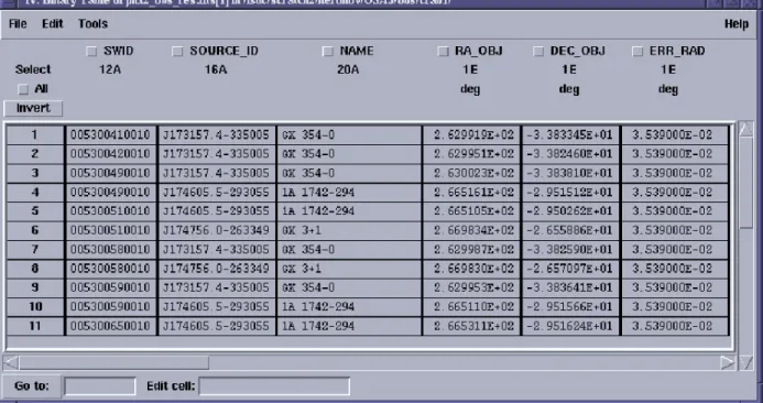
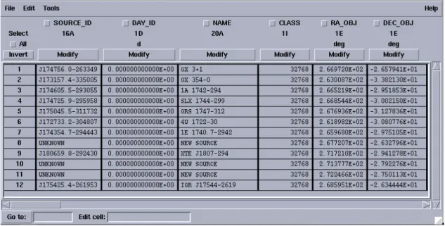
Apart from the mosaic images, the output of the IMA2 level contains a collection of the results from the individual science windows which is contained in the filejmx2 obs res.fits. Its content is shown in Fig.14. With the help ofcat2ds9command you can produce a region file found.regto locate these sources at the mosaic image:
cat2ds9 jmx2_obs_res.fits\[1] found.reg symbol=circle color=white
Note that since the same sources can be found in many ScWs you can have one and the same source repeated several times in the resulting region file.
You can look at the content of the resulting mosaic images contained in the filejmx2 mosa ima.fits with fv and display them withds9 exactly as you did with the images from individual ScWs (see Fig.15for the example of image in 7–11 keV energy band). In this figure you can see the sources found in single ScW analysis shown with white circles. One can see that two additional sources, which were not detected in the single ScWs, appear in the mosaic image (the sources shown by the green crosses).
If you are interested only in a particular region of the mosaic you can “zoom” on a given position in the sky running jemx science analysis with additional parameters IMA2 RAcenter, IMA2 DECcenter and IMA2 diameterwhich will specify the position of the center and the diameter (in degrees) of the resulting mosaic image. To do so, first move the existing images8:
mv jmx2_mosa_ima.fits jmx2_mosa_ima_original.fits mv jmx2_obs_res.fits jmx2_obs_res_original.fits
Remember that the images have to be also removed from the observation group. This can be done by the following command:
Figure 15:
The mosaic image of the Galactic Center region for revolution 0053 in the 7–11 keV energy band (sig-nifcance map).
dal_clean og_jmx2.fits+1
Now re-run the analysis script:
jemx_science_analysis startLevel="IMA2" endLevel="IMA2" jemxNum=2 \ IMA2_diameter=5.0 IMA2_RAcenter=266.4 IMA2_DECcenter=-29.0
(we have chosen to center the image on the Galactic Center position here).
If you want to produce a mosaic image only for a specific energy band you can pass the minimal and maximal energies of the selected energy band to thejemx science analysisthrough the parametersIMA2 eminSelect and IMA2 emaxSelect. Note that the energies have to be the same as defined previously in chanLowand chanHigh.
To get the largest possible output mosaic in equatorial coordinates the parameters ”radiusSelect” and ”di-ameter” must both be set to -1. A better way, available with OSA v.10.0, is to use the Aitoff-Hammer projection (in galactic coordinates) by setting the option AITproj. The latter enables the mosaicking of large parts of the sky, such as for the Galactic Plane Scans, without distortion of the map (an example is in Fig.16). This new feature can be activated setting the parameterIMA2_AITproj="yes". The command should be therefore as follows:
jemx_science_analysis startLevel="IMA2" endLevel="IMA2" jemxNum=2 IMA2_AITproj="yes"
The resultin