Automatic Extraction of Tempo and Beat from
Expressive Performances
Simon Dixon
Austrian Research Institute for Artificial Intelligence,
Schottengasse 3, Vienna 1010, Austria.
Email: [email protected]
Voice: +43-1-533 6112 22
Fax: +43-1-533 6112 77
August 27, 2001
Abstract
We describe a computer program which is able to estimate the tempo and the times of musical beats in expressively performed music. The input data may be either digital audio or a symbolic representation of music such as MIDI. The data is processed off-line to detect the salient rhythmic events and the timing of these events is analysed to generate hypotheses of the tempo at various metrical levels. Based on these tempo hypotheses, a multiple hypothesis search finds the sequence of beat times which has the best fit to the rhythmic events. We show that estimating the perceptual salience of rhythmic events significantly improves the results. No prior knowledge of the tempo, meter or musical style is assumed; all required information is derived from the data. Results are presented for a range of different musical styles, including classical, jazz, and popular works with a variety of tempi and meters. The system calculates the tempo correctly in most cases, the most common error being a doubling or halving of the tempo. The calculation of beat times is also robust. When errors are made concerning the phase of the beat, the system recovers quickly to resume correct beat tracking, despite the fact that there is no high level musical knowledge encoded in the system.
Introduction
The task of beat tracking or tempo following is perhaps best described by analogy to the human activities of foot-tapping or hand-clapping in time with music, tasks of which average human listeners are capable. Despite its apparent intuitiveness and simplicity compared to the rest of music perception, beat tracking has remained a difficult task to define, and still more difficult to implement in an algorithm or computer program. In this paper, we address the problem of beat tracking, and describe algorithms which have been implemented in a computer program for discovering the times of beats in expressively performed music.
The approach taken in this work is based on the belief that beat is a relatively low-level property of music, and therefore the beat can be discovered without recourse to high-level musical knowledge. It has been shown that even with no musical training, a human listener can tap in time with music (Drake et al., 2000). At the same time, it is clear that higher level knowledge aids the perception of beat. Drake et al. (2000) also showed that trained musicians are able to tap in time with music more accurately and require less time to synchronise with the music than non-musicians.
The primary information required for beat tracking is the onset times of musical events, and this is sufficient for music of low complexity and little variation in tempo. For more difficult cases, we show that a simple estimation of the salience of each musical event makes a significant improvement in the ability of the system to find beat times correctly.
Motivation and Applications
There are several areas of research for which this work is relevant, namely performance analysis, perceptual modelling, audio content analysis and synchronisation of a musical performance with computers or other devices.
Performance analysis investigates the interpretation of musical works, for example, the performer’s choice of tempo and expressive timing. These parameters are impor-tant in conveying structural and emotional information to the listener (Clarke, 1999). By finding the times of musical beats, we can automatically calculate the tempo and variations in tempo within a performance. This accelerates the analysis process, thus allowing more wide-ranging studies to be performed.
Perception of beat is a prerequisite to rhythm perception, which in turn is a funda-mental part of music perception. Several models of beat perception have been proposed (Steedman, 1977; Longuet-Higgins and Lee, 1982; Povel and Essens, 1985; Desain, 1992; Rosenthal, 1992; Parncutt, 1994; van Noorden and Moelants, 1999). Although this work is not intended as a perceptual model, it can inform perceptual models by examining the information content of various musical parameters, for example the re-lationship between the musical salience and the metrical strength of events.
Audio content analysis is important for automatic indexing and content-based re-trieval of audio data, such as in multimedia databases and libraries. This work is also necessary for applications such as automatic transcription or score extraction from per-formance data.
Another application of beat tracking is in the automatic synchronisation of devices such as lights, electronic musical instruments, recording equipment, computer anima-tion and video with musical data. Such synchronisaanima-tion might be necessary for mul-timedia or interactive performances or studio post-production work. The increasingly large amounts of data processed in this way leads to a demand for automatisation, which requires that the software involved operates in a “musically intelligent” way, and the interpretation of beat is one of the most fundamental aspects of musical intelli-gence.
Definitions of Terms
We assign the following meanings to terms used throughout the paper. Beat, as a phenomenon, refers to the perceived pulses which are approximately equally spaced and define the rate at which the notes in a piece of music are played. For a specific performance, the beat is defined by the occurrence times of these pulses (beat times), which are measured relative to the beginning of the performance.
A metrical level is a generalisation of the concept of the beat, corresponding to multiples or divisors of the beat which also divide the meter and any implied subdivi-sion of the meter evenly and begin on the first beat of the meter. For example, we can talk about the quarter note level of a piece in 3/4 or 4/4 meter, but not of a piece in 3/8 or 6/8 meter. Similarly, a piece in 4/4 meter has a half note level and a whole note
level, whereas a piece in 3/4 time has a dotted half note level. The primary metrical level is given by the denominator of the time signature (the notated level), which does
not necessarily equate to the perceptually preferred metrical level for the beat.
Score time is defined as the relative timing information derived from durations of
notes and rests in the score, measured in abstract units such as quarter notes and eighth notes. In conjunction with a metronome setting, score time can be converted to (nomi-nal) note onset times measured in seconds. The term performance time is used to refer to the concrete, measured, physical timing of note onsets. We defer discussion of the practical difficulties with the measurement of performance time until the section on evaluation.
A mechanical or metrical performance is a performance played strictly in score time. That is, all quarter notes have equal duration, all half notes are twice as long as the quarter notes, and so on. An expressive performance is any other performance, such as any human performance.
Tempo refers to the rate at which musical notes are played, expressed in score time
units per real time unit, for example quarter notes per minute. When the metrical level of the beat is known, the tempo can be represented by the number of beats per time unit (beats per minute is most common), or inversely as the inter-beat interval, measured in time per beat. Further, the tempo might be an instantaneous value, such as the inter-beat interval measured between two successive inter-beats, or an average tempo measured over a longer period of time. A measure of central tendency of tempo over a complete musical excerpt is called the basic tempo (Repp, 1994), which is the implied tempo around which the expressive tempo varies (not necessarily symmetrically).
Tempo induction is the process of estimating the basic tempo from musical data, and
a tempo hypothesis is one such estimate generated by the tempo induction algorithm shown in Figure 1. Beat tracking is the estimation of beat times based on a given tempo hypothesis. The term beat phase is used to refer to the times of musical events (or estimated beat times) relative to actual beat times.
Outline of Paper
In the background section, we review the literature on the modelling and analysis of tempo and beat in music, from score data, symbolic performance data and audio data, and conclude with a brief summary of models of performance timing and how they
relate to this work.
The following three sections give a detailed description of the algorithms used in tempo induction, beat tracking and calculating musical salience respectively. For tempo induction from audio data, the onsets of events are found using a time-domain method which seeks local peaks in the slope of the amplitude envelope. For symbolic perfor-mance data, the notes are grouped by temporal proximity into rhythmic events, and the salience of each event is estimated. The tempo induction algorithm then proceeds by calculating the inter-onset intervals between pairs of events (not necessarily adjacent), clustering the intervals to find common durations, and then ranking the clusters ac-cording to the number of intervals they contain and the relationships between different clusters, to produce a ranked list of basic tempo hypotheses. These hypotheses are the starting point for the beat tracking algorithm, which uses a multiple agent architecture to test the different tempo and phase hypotheses simultaneously, and finds the agent whose predicted beat times match most closely to those implied by the data. The eval-uation of agents is based on the assumption that the more salient events are more likely to occur in metrically strong positions. The estimation of musical salience is based on note duration, density, pitch and amplitude.
Evaluation of the system is then discussed, and a number of situations are presented in which the desired behaviour of a perfect beat tracking system is not clear. A practical methodology for evaluation is then described, including a formula for rating overall beat tracking performance on a musical work.
The results section begins with a brief description of the implementation details of the system, and then presents results for tempo induction and beat tracking of audio data, and then for symbolic data, using various measures of musical salience. We show that for popular music, which has a very regular beat, the onset times and amplitudes are sufficient for calculating beat times, but for music with greater expressive varia-tions, note duration becomes an important factor in being able to estimate beat times correctly.
The paper concludes with a discussion of the results obtained, the strengths and weaknesses of the system, and a preview of several possible directions of further work.
Background: Tempo Induction and Beat Tracking
Before discussing the methods, algorithms and results of the beat tracking system, we provide a brief background of previous work in the area. The literature on tempo induction and beat tracking is reviewed here in three parts, based on the type of in-put data. Firstly we examine models processing mechanical performances or musical scores, then we look at work involving symbolic performance data (usually MIDI), and finally we describe approaches to analysis of audio data. We conclude this section with a review of models of performance timing and discuss their relevance to beat tracking.
Scores and Mechanical Performance Data
For data with no expressive timing, the inter-beat interval is normally a multiple of the shortest duration, and all durations can be expressed in terms of rational multiples of
this interval. Research using this type of data usually goes beyond tempo induction, and tries to induce the complete metrical hierarchy.
Steedman (1977) describes a model of perception using note durations to infer ac-cents, and melodic repetition to infer metrical structure. He assumes that the meter is established clearly before any syncopation can occur, and therefore weights informa-tion at the beginning of a piece more highly than that which occurs later.
A model of rhythm perception developed by Longuet-Higgins and Lee (1982) pre-dicts beat times and revises the predictions in the light of the timing of events. For example, after the first two onsets are processed, it is predicted that the third onset will occur after an equal time interval so that the 3 events are equally spaced. If this expectation is fulfilled, the next expected interval is double the size of the previous interval. This method successfully builds binary hierarchies, but does not work for ternary meters. An extension of this work (Longuet-Higgins and Lee, 1984) provides a formal definition of syncopation and describes a preferred rhythmic interpretation as one which avoids syncopation.
Lerdahl and Jackendoff (1983) describe meter perception as the process of finding periodicities in the phenomenal and structural accents in a piece of music. They pro-pose a set of metrical preference rules, based on musical intuitions, which are assumed to guide the listener to plausible interpretations of rhythms. The rules prefer structures where: beats coincide with note onsets; strong beats coincide with onsets of long notes; parallel groups receive parallel metrical structure; and the strongest beat occurs early in the group.
Povel and Essens (1985) propose a model of perception of temporal patterns, based on the idea that a listener tries to induce an internal clock which matches the distribution of accents in the stimulus and allows the pattern to be expressed in the simplest possible terms. They use patterns of identical tone bursts at precise multiples of 200ms apart to test their theory. They do not suggest how the theory should be modified for musical data or non-metrical time.
A theoretical and experimental comparison of the above models is reported by Lee (1991). He concludes that every meter has a canonical accent pattern of strong and weak beats, and that listeners induce meter by matching the natural accent patterns occurring in the music to the canonical accent pattern of possible rhythmic interpreta-tions. In this model, major syncopations and weak long notes are avoided.
Desain and Honing (1999) compare several tempo induction models, integrating them into a common framework and showing how performance can be improved by optimisation of the parameters.
Symbolic Performance Data
Much of the work in machine perception of rhythm has used MIDI files as input (Rosenthal, 1992; Rowe, 1992; Desain, 1993; Large, 1995; Cemgil et al., 2001).
The input is usually interpreted as a series of event times, ignoring the event dura-tion, pitch, amplitude and chosen synthesizer voice. That is, each note is treated purely as an uninterpreted event. It is assumed that the other parameters do not provide
doubt that these factors provide useful rhythmic cues; for example, more salient events tend to occur on stronger beats.
Notable work using MIDI file input is Rosenthal’s emulation of human rhythm perception (Rosenthal, 1992), which produces multiple hypotheses of possible hierar-chical structures in the timing, assigning a score to each hypothesis, corresponding to the likelihood that a human listener would choose that interpretation of the rhythm. This technique gives the system the ability to adjust to changes in tempo and meter, as well as avoiding many implausible rhythmic interpretations.
A similar approach is advocated by Tanguiane (1993), using Kolmogorov complex-ity as the measure of the likelihood of a particular interpretation, with the least complex interpretations being favoured. He provides an information-theoretic account of human perception, and argues that many of the “rules” of music composition and perception can be explained in information-theoretic terms.
Desain (1993) compares two different approaches to modelling rhythm perception, the symbolic approach of Longuet-Higgins (1987) and the connectionist approach of Desain and Honing (1989). Although this work only models one aspect of rhythm per-ception, the issue of quantisation, and the results of the comparison are inconclusive, it does highlight the need to model expectancy, either explicitly or implicitly. Expectancy is a type of predictive modelling relevant to real time processing, which provides a con-textual framework in which subsequent rhythmic patterns can be interpreted with less ambiguity.
Allen and Dannenberg (1990) propose a beat tracking system that uses beam search to consider multiple hypotheses of beat timing and placement. A heuristic evalua-tion funcevalua-tion directs the search, preferring interpretaevalua-tions that have a “simple” musical structure and make “musical sense”, although these terms are not defined. They also do not describe the input format or any specific results.
Large and Kolen (1994); Large (1995, 1996) use a nonlinear oscillator to model the expectation created by detecting a regular pulse in the music. The system does not perform tempo induction; the basic tempo and initial phase must be supplied to the sys-tem, which then tracks tempo variations using a feedback loop to control the frequency of the oscillator. On improvised melodies, the system achieved a mean absolute phase error of under 10% for most data, which was considered subjectively good.
Another system which uses multiple hypotheses is from Rowe (1992), who dis-cretises the complete tempo range into 123 inter-beat intervals ranging from 280ms to 1500ms in 10ms steps, corresponding to metronome markings of 40–208 beats per minute. Each tempo theory tries to provide a plausible rhythmic interpretation for in-coming events, and the most successful theories are awarded points. The system copes moderately well with simple input data, but cannot deal with complex rhythms.
An alternative approach is to model tempo tracking in a probabilistic framework (Cemgil et al., 2001). The beat times are modelled as a dynamical system with variables representing the rate and phase of the beat, and corresponding to a perfect metronome corrupted by Gaussian noise. A Kalman filter is then used to estimate the unknown variables. Since the beat times are not directly observable from the data, they are induced by calculating a probability distribution for possible interpretations of perfor-mances. The system parameters are estimated by training on a data set for which the correct beat times are known. The system performs well (over 90% correct) on a large
number of performances of a simple arrangement of a popular song. The results are compared with the current system in Dixon (2001a).
Audio Data
The earliest work on automatic extraction of rhythmic content from audio data is found in the percussion transcription system of Schloss (1985). Onsets are detected as peaks in the slope of the amplitude envelope, where the envelope is defined to be equal to the maximum amplitude in each period of the high-pass filtered signal, and the period defined as the inverse of the lowest frequency expected to be present in the signal. The main limitation of the system is that it requires parameters to be set interactively. Also, no quantitative evaluation was made; only subjective testing was performed, by resynthesis of the signal.
The main work in beat tracking of audio data is by Goto and Muraoka (1995, 1997a,b, 1998, 1999) who developed two beat tracking systems for popular music, the first for music containing drums and the second for music without drums. The earlier system (BTS) examines the frequency bands centred on the frequencies of the snare and bass drums, and matches the patterns of onset times of these two drum sounds to a set of pre-stored drum patterns. This limits the system to a very specific style of music, but the beat tracking on suitable songs is almost always successful.
Goto and Muraoka’s second system makes no assumption about drums; instead, it uses frequency-domain analysis to detect chord changes, which are assumed to occur in metrically strong positions. This is the first system to demonstrate the use of high level knowledge in directing the lower-level beat tracking process. The high level knowledge is specific to the musical style, which is a major limitation of the system. Furthermore, all music processed by the system is assumed to be in 4/4 time, with a tempo between 61 and 120 quarter note beats per minute, chord changes occurring in strong metrical positions (not every beat), and no tempo changes.
Both systems are based on a multiple agent architecture using a fixed number of agents (28 and 12 in the two systems, respectively). Each agent predicts the beat times using different strategies (parameter settings). One feature of this work which does not appear in most beat tracking work is that three metrical levels (quarter note, half note and whole note) are tracked simultaneously. The system also operates in real time, for which it required a multiple-processor computer at the time it was built. (A fast personal computer today has almost the same computing power.)
Scheirer (1998) also describes a system for the beat tracking of audio signals, based on tuned resonators. The signal is split into 6 frequency bands, and the amplitude envelopes in each band are extracted, differentiated and rectified before being passed to a bank of 150 comb filters (representing each possible tempo on a discretised scale). The output of the filters is summed across the frequency bands, and the maximum output gives the tempo and phase of the signal. The system was evaluated qualitatively on short musical excerpts from various styles, and successfully tracked 41 of the 60 examples. One problem with the system is that in order to track tempo changes, the system must repeatedly change its choice of filter, which implies the filters must be closely spaced to be able to smoothly track tempo variations. However, the system applies no continuity constraint when switching between filters.
Two recent approaches which find periodicities in audio data have been proposed (Cariani, 2001; Sethares and Staley, 2001). Cariani (2001) presents a neurologically plausible model called a recurrent timing net (RTN). The audio data is preprocessed by finding the RMS amplitude in overlapping 50ms windows of the signal, and the result-ing data is passed to the RTN, which effectively computes a runnresult-ing autocorrelation at all possible time lags in order to find the most significant periodicities in the data. Sethares and Staley (2001) filter the audio signal into 1/3 octave bands, decimate to a low sampling rate and then search for periodicities using the periodicity transform de-veloped previously in (Sethares and Staley, 1999). Although both of these approaches use audio input, they assume constant tempo performances, and so are not directly relevant to the analysis of expressive performance.
Modelling of Performance Timing
An understanding of rules governing expressive timing is advantageous in develop-ing a system to follow tempo changes. Technical advances over the last decades have facilitated the analysis of timing in music performance in ways that were previously infeasible. Clarke (1999) and Gabrielsson (1999) review research in this area and con-clude that expressive timing is generated from the performers’ understanding of the musical structure and general knowledge of music theory and musical style. However, there is no precise mathematical model of expressive timing, and the complexity of musical structure from which timing is derived, coupled with the individuality of each performer and performance, makes it impossible to capture musical nuance in the form of rules. Attempts to formulate rules governing the relationship between the score and expressive timing (Todd, 1985; Clarke, 1988; Friberg, 1995) are partially successful, as judged by listening tests and by comparison with performance data, but ignore individ-ual performers’ interpretation and cover only limited aspects of musical performance.
Tempo Induction
The beat tracking system has two stages of processing, the initial tempo induction stage, which is described in this section, and the beat tracking stage, which appears in the following section. The tempo induction stage examines the times between pairs of note onsets, and uses a clustering algorithm to find significant clusters of inter-onset intervals. Each cluster represents a hypothetical tempo, expressed as an inverse value, the inter-beat interval, measured in seconds per beat. The tempo induction algorithm ranks each of the clusters, with the intention that the most salient time intervals are ranked most highly. The output from this stage (and input to the beat tracking stage) is the ranked list of tempo hypotheses, each representing a particular beat rate, but saying nothing about the beat times (or beat phase), which are calculated in the subsequent beat tracking stage.
The tempo induction algorithm operates on rhythmic events, an abstract representa-tion of the performance data as a weighted sequence of time points. A rhythmic event may represent the onset of a single note or a collection of notes played approximately simultaneously. Events are characterised by their onset time and a salience value which
is calculated from the parameters of the constituent notes of the event, such as pitch, loudness, duration, and number of constituents. We now describe the various input data formats, and then the generation of the rhythmic event representation of performance data, and finally present the tempo induction algorithm based on this representation.
Input Data
There are two types of input data accepted by the beat tracking system: digital audio and symbolic performance representations, which are described in turn.
There are a large number of digital audio formats currently in use, which provide various possible representations of the audio data, allowing the user to choose the bit rate and/or compression algorithm suitable for the task at hand. Considering the wide availability of software for converting between formats, we limited the input data for-mat to uncompressed linear pulse code modulated (PCM) signals, as found on compact discs and often used in computer audio applications. The specific file format may be either the MS “.wav” format or SUN “.snd” format, both of which permit choices of sampling rates, word sizes and numbers of channels. For the results reported in this paper, single channel 16 bit linear PCM data was used, with a sampling rate of 44100 Hz. This data was created directly from compact discs by averaging the two channels of the original stereo recordings.
Two symbolic formats may be used, MIDI, the almost universal format for sym-bolic performance data, and the Match format, a locally developed text format com-bining the representation of MIDI performance data with the musical score, and as-sociating the corresponding notes in each. The Match format facilitates the automatic evaluation of the beat tracking results relative to the musical score.
Rhythmic Events
Rhythmic information is primarily carried by the onset times of musical components (musical notes and percussive sounds). When these components have onset times which are sufficiently close together, they are heard as a composite event, which we name a rhythmic event. A rhythmic event is characterised by an onset time and a salience. Rhythmic events represent the most basic unit of rhythmic information, from which all beat and tempo information is derived. The process of deriving the rhythmic events from symbolic data is entirely different from that required for audio data, as most of the required information is directly represented in the symbolic data, whereas it must be estimated by an imperfect onset detection algorithm in the audio case. Symbolic Data
For symbolic representations, the onset time of each musical note is encoded directly in the data. This onset time denotes the beginning of the waveform, not the perceived onset time, which usually falls slightly later, depending on the rise time of the instru-ment (Vos and Rasch, 1981; Gordon, 1987). With symbolic data, it is not possible to correct for the instrumental rise time, because the waveform is not encoded in the data,
and thus is unknown. However, since most rhythmic information is carried by percus-sive instruments or other instruments with very short rise times, this does not create a noticeable problem.
The first task which must be performed is to group any approximately simultaneous onsets into single rhythmic events, and calculate the salience of each of the rhythmic events. In studies of chord asynchrony in piano and ensemble performance, it has been shown that asynchronies of 30–50ms are common, and much larger asynchronies also occur (Sundberg, 1991; Goebl, 2001). Perception research has shown that with up to 40ms difference in onset times, two tones are heard as synchronous, and for more than two tones, the threshold is up to 70ms (Handel, 1989). In this work, a threshold of 70ms was chosen for grouping near onsets into single rhythmic events.
The second task is to calculate the salience of the rhythmic events. Music theory identifies several factors which contribute to the perceived salience of a note. We par-ticularly focus on note duration, density, dynamics and pitch in this work, since these factors are represented in the MIDI and Match file data. The precise way in which these factors are combined to give a numerical salience value for each rhythmic event is described later.
Audio Data
Audio data requires significant processing in order to extract any symbolic information about the musical content of the signal. To date, no algorithm has been developed which is capable of reliably extracting the onset times of all musical notes from audio data. Nevertheless, it is possible to extract sufficient information in order to perform tempo induction and beat tracking. In fact, beat tracking may be improved by a lossy onset detection algorithm, as it implicitly filters out the less salient onsets (Dixon, 2000).
The onset detection method is based loosely on the techniques of Schloss (1985), who analysed audio recordings of percussion instruments in order to transcribe perfor-mances. The signal is passed through a first order high pass filter, and then smoothed to produce an amplitude envelope. The amplitude envelope is calculated as the average absolute value of the signal within a window of the signal. In this work a window of 20ms was used, with a 50% overlap, so that smoothed amplitude values were calculated at 10ms intervals. A 4-point linear regression is used to find the slope of the amplitude envelope, and a peak-picking algorithm then finds local maxima in the slope of the amplitude envelope. Local peaks are rejected if there is a greater peak within 50ms, or if the peak is below threshold (10% of the average amplitude per 10ms). The default parameter values as used in this work were determined empirically, but all values can be adjusted via command-line parameters.
For tasks such as transcription, it is important that all onsets are found, and the present time-domain technique would not suffice – it would be necessary to use a fre-quency domain method to detect onsets more reliably. However, for beat tracking, it is advantageous to discover just the most salient onsets, as these are more likely to correspond to beat times. In other words, the onset detection algorithm performs an implicit filtering of the true onsets, removing those with a low salience. The actual salience value for the detected peaks, used later in the beat tracking algorithm, is a
linear function of the logarithm of the amplitude envelope value.
The onset detection algorithm has not been tested for music without instruments with sharp rise times; we expect that in this case a frequency domain algorithm would be required to find onsets sufficiently reliably.
Clustering of Inter-Onset Intervals
Once the rhythmic events have been determined, the time intervals between pairs of events reveal their rhythmic structure. The clustering algorithm (Figure 1) uses this data to generate a ranked list of tempo hypotheses, which are then used as the basis for beat tracking. In the literature, an inter-onset interval (IOI) is defined as the time between two successive events. We extend the definition to include compound intervals, that is intervals between pairs of events which are separated by other events. This is important in reducing the effect of any events which are uncorrelated with the beat.
Rhythmic information is provided by IOIs in the range of approximately 50ms to 2s (Handel, 1989). The clustering algorithm assigns each IOI to a cluster of similar intervals, if one exists, or creates a new cluster for the IOI if no sufficiently similar cluster exists. The clusters are characterised by the average of the IOIs contained in the cluster, which we denote the interval of the cluster. Similarity holds if the given IOI lies within a small distance (called the cluster width) of the cluster’s interval. The cluster width is kept small (in this work 25ms) so that outlying values do not affect the cluster’s interval. Nevertheless, the incremental building of the clusters means that the interval of a cluster can drift as IOIs are added.
Once cluster formation is complete, pairs of clusters whose intervals have drifted together are merged, and the clusters are ranked according to the number of elements they contain, with an adjustment for any related clusters. Two clusters are said to be related if the interval of one cluster is within the cluster width of an integer multiple of that of the other cluster. This reflects the expectation that for a cluster representing the beat, there will also exist clusters representing integer multiples and integer divisions of the beat. The adjustment is applied to the cluster’s interval by calculating the average of the related clusters’ normalised intervals, weighted by their scores. The ranking of the clusters is also adjusted by adding the scores of related clusters, weighted by a relationship factor
, where
is the integer ratio of cluster intervals, given by:
! "$#&%('*),+.-0/$'
The top ranked clusters represent a set of hypotheses as to the basic tempo of the music. At this point it is not necessary to choose between hypotheses; this choice is made later by the beat tracking algorithm. The clustering algorithm is usually suc-cessful at ranking the primary metrical level as one of the highest ranking clusters (see results section). What the clustering algorithm does not provide is any indication of the beat times. This task is performed by the beat tracking stage described in the next section.
Definitions
Events are denoted by12
143
1.5 *67676
The inter-onset interval between events198 and1;: is denoted by<=><*8?: Clusters are sets of inter-onset intervals denoted by@42
@;3 @A5 *676B6 @A8.interval
DCFEHGIKJMLONLEHGIQPR(ST
U
R
S
U
WV
is the relationship factor -&YXZQ[(&\]&V
are positive integer variables Algorithm
FOR each event198 FOR each event1A:
<=><*8?: _^ 1;: .onset 198.onset ^ Find[ such that^ @;` .interval <=><*8?: ^ba ClusterWidth is minimum IF[ exists THEN @;`dc @e`efhg$<=><*8?:,i ELSE
Create new cluster@Ajkc gl<=><*8?:,i END IF
END FOR END FOR
FOR each cluster@A8 FOR each cluster@:
7Xhm n-0 IF ^ @A8.interval @o: .interval ^ba ClusterWidth THEN @p8qc @A8rfs@: Delete cluster@: END IF END FOR END FOR
FOR each cluster@A8 FOR each cluster@:
IF ^ @A8.interval Vut @: .interval ^ba ClusterWidth THEN @p8.scorec @p8.score + WVvt @: .size END IF END FOR END FOR
Time Events IOI’s A B C D E C1 C1 C2 C1 C2 C3 C3 C4 C4 C5
Figure 2: Clustering of inter-onset intervals (IOI’s)
Example
We illustrate the tempo induction stage with a short example. Consider the sequence of five eventsw
Mx
@
Oyh
1 shown on the time line in Figure 2. Below the time line, the horizontal lines with arrows represent each of the inter-onset intervals between pairs of events, and these lines are labelled with the name of the cluster to which they are assigned. Five clusters are created, denoted C1, C2, C3, C4 and C5, with C1
g$w xMx @ My 1zi , C2 g{w@ @ y i , C3 g x|y} @1i , C4 g$w y}Mx 1zi and C5 g{w41zi . The scores for each cluster are calculated as follows:
C1.score = 2*3*f(1) + 2*f(2) + 2*f(3) + 2*f(4) + f(5) = 49
C2.score = 3*f(2) + 2*2*f(1) + 0 + 2*f(2) + 0 = 40
C3.score = 3*f(3) + 0 + 2*2*f(1) + 0 + 0 = 29
C4.score = 3*f(4) + 2*f(2) + 0 + 2*2*f(1) + 0 = 34
C5.score = 3*f(5) + 0 + 0 + 0 + 2*1*f(1) = 13
Therefore the clusters are ranked in the following order: C1, C2, C4, C3, C5.
Beat Tracking
The Beat Tracking Architecture
The tempo induction algorithm computes the approximate inter-beat interval, that is, the time between successive beats, but does not calculate the beat times. In Figure 2, for example, one hypothesis might be that C2 represents the inter-beat interval, but it does not determine whether events A, C and D are beat times or whether B, E and the midpoint of BE are beat times. That is, tempo induction calculates the beat rate (frequency), but not the beat time (phase).
In order to calculate beat times, a multiple hypothesis search is employed, with an evaluation function selecting the hypothesis that fits the data best. Each hypothesis is handled by a beat tracking agent, which is able to predict beat times and match them to rhythmic events, adjust its hypothesis of the current beat rate and phase, create a new
agent when there is more than one reasonable path of action, and cease operation if it is found to be duplicating the work of another agent.
Each agent is characterised by its state and history. The state is the agent’s current hypothesis of the beat frequency and phase, and the history is the sequence of beat times selected to date by the agent. The agents can also assess their performance, by evaluating the goodness of fit of the tracking decisions to the data.
The system is designed to track smooth changes in tempo and small discontinuities; the choice of a single best agent based on its cumulative score for beat tracking the whole piece means that a piece which changes its basic tempo significantly will not be tracked correctly. In future work we plan to examine a real time approach to beat tracking, using an incremental tempo induction algorithm; at each point in time the best agent is chosen based on a combined score for its tempo and the tracking of music up to that time, thus allowing sudden changes in tracking behaviour when the previous best agent ceases to be able to track the data correctly.
The Beat Tracking Algorithm
The beat tracking algorithm is given in full in Figure 3. This algorithm is now explained in detail, with reference to the example shown in Figure 4.
Initialisation
For each hypothesis generated by the tempo induction phase, a group of agents are created to track the piece at this tempo. Based on the assumption that at least one event in the initial section of the music coincides with a beat time (normally there will be many events satisfying this condition), an agent is created for each event in the initial section, with its first beat time coinciding with that of the respective event. Using this approach, it is usually the case that there is an agent that begins with the correct tempo and phase.
The initial section, as defined by the constant StartupPeriod in the algorithm, was set to be the first 5 seconds of the music. In some cases, for example when a piece has a free-time introduction, it is possible that no agent starts with the correct tempo and phase. However, an agent with approximately the correct tempo will be able to adjust its tempo and phase in order to synchronise with the beat.
In Figure 4, a simplified example illustrates the operation of the beat tracking algo-rithm. The rhythmic events (denoted A, B, C, D, E and F) are represented on the time line at the top of the figure. The beat tracking behaviour of each agent is represented by the horizontal lines connecting filled and hollow circles. The filled circles represent beat times which correspond to a rhythmic event, and the hollow circles are beat times which were interpolated because no rhythmic event occurred at that time.
The figure illustrates 2 tempo hypotheses from the tempo induction stage. The faster tempo, with an inter-beat interval approximately equal to the time interval be-tween events A and B, is the tempo hypothesis of Agent1. The slower tempo, with inter-beat interval approximately equal to the interval between C and D, is the tempo hypothesis of the other agents. For the initialisation stage, assume that only events A and B are in the initial section, and then nominally it is expected that 4 agents would
Initialisation
FOR each tempo hypothesis~r8 FOR each event1;: such that1;:
6
onseta
StartupPeriod Create a new agentw`
w`
6
beatIntervalc ~r8 w`
6
predictionc 1A: .onset4~r8 w` 6 historyc 1;:K w` 6 scorec 1;: 6 salience END FOR END FOR Main Loop FOR each event198
FOR each agentwe: IF198 6 onset we: 6
history.last TimeOut THEN Delete agentwe:
ELSE WHILEwe: 6 prediction.~ "{ $MHpa 198 6 onset we: 6 predictionc we: 6 prediction4we: 6 beatInterval END WHILE IFwe: 6 prediction.~ "{ *Oe 198 6 onset we: 6 prediction.~ "{ $&Y THEN IF ^ we: 6 prediction 198 6 onset^ ~ "{ 8 Y Create new agentw`dc we:
END IF Errorc 198 6 onset we: 6 prediction we: 6 beatIntervalc we: 6
beatInterval Error CorrectionFactor we: 6 predictionc 198 6 onsetwe: 6 beatInterval we: 6 historyc we: 6 history1e8 we: 6 scorec we: 6 score relativeError vt 198 6 salience END IF END IF END FOR
Add newly created agents Remove duplicate agents END FOR
Return the highest scoring agent
Time Events A B C D E F Agent1 Agent2 Agent2a Agent3
Figure 4: Beat tracking by multiple agents
Time
Events A B C D
Inner windows: Outer windows:
Figure 5: Tolerance windows for beat tracking
be created, one for each (tempo hypothesis, initial event) pair. In fact, only 3 agents are created, Agent1 with the faster tempo, and Agent2 and Agent3 with the slower tempo. This is because the system recognises that a fast tempo agent beginning on event B would be redundant, since Agent1 also predicts B as a beat time.
Main Loop
In the main body of the beat tracking algorithm, each event is processed in turn by allowing each agent the opportunity to consider the event as a beat time. Each agent has a set of predicted beat times, which are generated from the most recent beat time by adding integer multiples of the agent’s current inter-beat interval. These predicted beat times are surrounded by two-level windows of tolerance, which represent the extent to which an agent is willing to accept an alteration to its prediction (see Figure 5). The inner window, set at 40ms either side of the predicted beat time, represents the deviations from strict metrical time which an agent is willing to accept. The outer window, with a default size of 20% and 40% of the inter-beat interval respectively before and after the predicted beat time, represents changes in tempo and/or phase which an agent will accept as a possibility, but not a certainty. The asymmetry reflects the fact that expressive reductions in tempo are more common and more extreme than tempo increases (Repp, 1994).
There are three possible scenarios when an agent processes an event, illustrated in Figure 4. The simplest case is when the event falls outside the tolerance windows of predicted beat times, and the event is ignored. For example, in the figure, event D is ignored by Agent1 and Agent3, and event B is ignored by Agent2. The second case is when the event falls in the inner tolerance window of a predicted beat time, so that the event is accepted as a beat time. Event B with Agent1 and events D and E with Agent2
are examples of this case. If the event is not in the first predicted beat window, then the missing beats are interpolated by dividing the time interval into equal durations, as shown by the hollow circles in the figure. For example, this occurs at events C, E and F for Agent1 and event E for Agent3. The agent’s tempo is then updated by adjusting the tempo hypothesis by a fraction of the difference between the predicted and chosen beat times, and the score is updated by adding the salience of the event, which is also adjusted (downward) according to the difference between predicted and chosen beat times. The third and most complex case is when the event falls in one of the outer tolerance windows. In this case, the agent accepts the event as a beat time, but as insurance against a wrong decision, also creates a new agent that does not accept the event as a beat time. In this way, both possibilities can be tracked, and the better choice is revealed later by the agents’ final scores. This is illustrated in Figure 4 at event E, where Agent2 accepts the event and at the same time creates Agent2a to track the possibility that E is not a beat time.
Complexity Management
Since each agent’s future beat tracking behaviour is entirely based on its current state (tempo and phase) and the input data, any two agents that agree on the tempo and phase will exhibit identical behaviour from that time on, wasting computational resources. In order to increase efficiency, the duplicate agents are removed at the earliest opportunity. Theoretically, such an operation should make no difference to the results produced by the system, but one complication arises, that the tempo and phase variables are continuous, so equality is too strong a condition to use in comparing agents’ states. Therefore thresholds of approximate equality were chosen, conservatively, at 10ms for the inter-beat interval (tempo) difference and 20ms for the predicted beat time (phase) difference.
When the decision to remove a duplicate agent is made, it is important to consider which agent to remove. The agents have different histories (otherwise the duplicate would have been removed sooner), and therefore different evaluation scores. Since the evaluation is calculated based only on the relationship between predicted beat times and the rhythmic events, and not on any global measure of consistency, it is always correct to retain only the agent with the higher current score, since it will also have the higher total score at the end of beat tracking. In Figure 4, Agent3 is deleted after event E, because it agrees in tempo and phase with Agent2. This is indicated by the arrow between Agent3’s and Agent2’s event E.
Assessment
The comparison of the agents’ beat tracking is based on three factors: how evenly spaced the chosen beat times are, how often the beat times match times of rhythmic events, and the salience of the matched rhythmic events. As stated above, the evenness of beat times is not calculated via a global measure, but from the local agreement of predicted beat times and rhythmic events.
For each beat time at which a rhythmic event occurs, a fraction of the event’s salience is added to the agent’s score. The fraction is calculated from the relative error
of the predicted beat time; that is the difference in predicted and chosen beat times, divided by the window half-width, which is then halved and subtracted from 1. This gives a score between 0.5 and 1.0 times the salience for each event. The beat tracking algorithm then returns the agent with the greatest score.
Estimating Musical Salience
In earlier work (Dixon, 2000), where it was assumed that expressive variations in tempo were minimal, it was found that no specific musical knowledge was needed by the sys-tem in order to perform beat tracking successfully. That is, by searching for a regularly spaced subset of the events with few gaps and little variation in the spacing, the system was able to find the times of beats. As the system was tested with more expressive mu-sical examples, it was found that the search had to allow greater variation in the beat spacing, which led to an increase in the number of choices, and therefore the number of agents. Without further musical knowledge, it was not possible for the system to choose correctly between the many possible musical interpretations offered by the var-ious agents. In this section we describe how knowledge of musical salience was added to the system in order to direct the system to the more plausible musical interpretations (Dixon and Cambouropoulos, 2000).
When comparing beat tracking results for audio and MIDI versions of the same performances, it was discovered that the onsets extracted from audio data, although unreliable, provided a better source of data for beat tracking than the onset times ex-tracted without error from the MIDI data. It was postulated that this was due to an implicit filtering of the data. That is, only the more significant onsets had been ex-tracted; the less salient onsets remained undetected, and had no influence on the beat tracking system. The reason this was advantageous is that the more salient events are more likely to correspond to beat times than the less salient events, and hence the search had been narrowed by the onset detection algorithm.
This hypothesis is tested by incorporating knowledge of musical salience into the system, and measuring the corresponding performance gain. This is done using MIDI data, since parameters such as duration, pitch and volume, which are important deter-miners of salience, are all directly available from the data.
Observations From Music Theory
The tendency for events with greater perceptual salience to occur in stronger metrical positions has been noted by various authors (Longuet-Higgins and Lee, 1982; Lerdahl and Jackendoff, 1983; Povel and Essens, 1985; Lee, 1991; Parncutt, 1994). The factors influencing perceived salience have also been studied, although no model has been proposed which predicts salience based on combinations of factors, or which gives more than a qualitative account of the effects of parameters.
Lerdahl and Jackendoff (1983) classify musical accents into three types: phenom-enal accents, which come from physical attributes of the signal such as amplitude and frequency; structural accents, which arise from perceived points of arrival and depar-ture such as cadences; and metrical accents, points in time which are perceived as
ac-cented due to their metrical position. We only concern ourselves with the first type of accent here, since the higher level information required for the other types is not avail-able to the beat tracking system. Lerdahl and Jackendoff list the following types of phenomenal accent (which they consider incomplete): note onsets, sforzandi, sudden dynamic or timbral changes, long notes, melodic leaps and harmonic changes. How-ever, they give no indication as to how these factors might be compared or combined, either quantitatively (absolute values) or qualitatively (relative strengths).
In other models of meter perception, the main factor determining salience is note duration, which is usually taken to mean inter-onset time rather than perceived or phys-ical sounding time of a note. For example, Povel and Essens (1985) describe three scenarios in which a note receives a perceived accent relative to other notes of identi-cal pitch, amplitude envelope and physiidenti-cal duration. In their model, notes which are equally spaced in time form groups, subject to the condition that there are no notes outside the group which are closer to any note in the group. Then the notes which receive accents are: notes which do not belong to any group, the second note of any group of two notes, and the first and last note of any group of three or more notes. All of these accents, except the first note in groups of 3 or more, fall on notes with a long duration relative to their context. Other authors (Longuet-Higgins and Lee, 1982; Parncutt, 1987; Lee, 1991) also state that longer notes tend to be perceived as accented. All of the models based on inter-onset times were developed in a monophonic con-text, and are difficult to interpret when considering the polyphonic context of most musical performances. For example, one would intuitively expect that a long note in a melody part should not lose its accent due to notes in the accompaniment which fol-low shortly after the onset of the melody note. However, if we were to observe the inter-onset times only, this would be the result of such models. To adapt to polyphonic music, a model of auditory streaming (Bregman, 1990) could be applied, so that inter-actions between streams are removed, but that raises the difficult question of how the metrical perception of the various streams could be combined into a single percept. A simpler approach is to use the physical durations of notes rather than inter-onset times, even though these are difficult to estimate from audio data.
Combining Salience Factors
For this work, the factors chosen as determiners of musical salience were note duration, simultaneous note density, note amplitude and pitch, all of which are readily available in the symbolic representation of the performance. The next task was the combination of these factors into a single numerical value, representing the overall salience of each rhythmic event. None of the above-mentioned work has investigated or proposed a method of combining salience, so it was decided to test two possible salience models by their influence on the beat tracking results. The two models presented are a linear combination/lKQbM
of duration , pitch
and amplitude
, and a nonlinear, mul-tiplicative function/
j;, v&F
of the same parameters. A threshold function is used to restrict the values of
to a limited range, and constants are used to set the relative weights of the parameters. The salience of a group of notes combined as a single rhyth-mic event was calculated using the longest duration, the sum of the dynarhyth-mic values and the lowest pitch of all the notes in the group.
The salience functions were defined as follows: /lKObv&Fq 2 6 3 6 j;87 j K 5 6 / jA FMq 6Q j;87 j K O6"* ¡W where: 2 Q 3 O 5 and O are constants, is duration in seconds,
is pitch (MIDI number),
is dynamic value (MIDI velocity), and
j;87 j K j;87 ¢}] j;87 j;87 a£ha£ j K j KD j Kz]
The following weights for the parameters were determined empirically:
2 ¤ !! 3 5 k O4 , j;87 nb j K| ¦¥
These values make duration the most significant factor, with dynamics and pitch being useful primarily to distinguish between notes of similar duration. This salience calcu-lation is not sufficient for all possible MIDI files. In particular, it would not work well for non-pitched percussion such as drums, where the salience is clearly not so strongly related to duration. Such instruments should be treated separately as a special case of the salience calculation.
We will now describe the task of evaluating the beat tracking system, before pre-senting the results in the following section.
Evaluation
We know of no precise definition of beat for expressively performed music. The defini-tions given in the first section of the paper do not uniquely define the relevant quantities or give a practical way of calculating them from performance data. In this section, we describe the difficulties with formalisation and evaluation of beat tracking models and systems, and then describe the evaluation methodology used in this work.
Problems with Evaluation
The tempo induction and beat tracking algorithms described in this paper were not designed for any particular style of music. They operate in the same way for classical music played from a score as for improvised jazz. This immediately creates a difficulty for evaluation, in that we cannot assume that a musical score is available to define which notes coincide with beats and which do not. It is laborious (but possible) for a trained musician to transcribe a performance in enough detail to identify which notes occur on the beat. But even when a score or transcription exists, there is no error-free, automatic way to associate the score timing with the performance timing of audio data. That is, given a score, we can establish which notes in the score correspond to beat times, but we do not know the absolute times of score notes, and the beat tracking system returns its results as absolute times. The accurate extraction of onset times in polyphonic music is an unsolved problem, so we are forced to rely on hand-labelled or hand-corrected data for evaluation purposes. This issue is discussed in much greater detail by Goto and Muraoka (1997a), who also use a similar approach to that which we describe below.
Further problems exist which apply equally to audio and symbolic performance data. There are many cases in which the beat is not uniquely defined by performance data. In the simplest case, consider a chord which occurs on a beat according to the score. In performance, it has been observed that the notes of a chord are not necessar-ily played simultaneously, and these asynchronies may be random or systematic (e.g. melody lead) (Palmer, 1996; Repp, 1992; Goebl, 2001). The problem is more pro-nounced in ensemble situations, where there are often systematic timing differences between performers (participatory discrepancies) (Keil, 1995; Prögler, 1995; Gabriels-son, 1999).
It is not obvious how the beat time should then be defined, whether at the onset of the first note of the chord, or of the last, the lowest, or the highest, or at the (weighted) average of the onset times, or alternatively expressed as a time interval. The problem is exacerbated in situations where timeless events are notated, such as grace notes and arpeggios. Performers may interpret grace notes in different ways, sometimes to pre-cede the beat, and sometimes to coincide with the beat. In some cases hearers do not even agree on which interpretation they think the performer applied.
It is reasonable to question whether beats necessarily correspond to event times. A beat percept induced by previous events might be stronger than that of an event which nominally coincides with the beat, and in this case the event is perceived as anticipating or following the beat rather than defining the beat time.
The point of this section is to show that some subjective judgement is necessary in evaluating the results produced by a beat tracking program. Our aim is to keep this sub-jectivity to a minimum, and define an evaluation methodology which gives repeatable results. We distinguish between two approaches to beat tracking: predictive (percep-tual) and descriptive beat tracking. An algorithm is said to be causal if its output at time
#
depends only on input data for times#
. Predictive beat tracking models perception using causal algorithms which predict listeners’ expectations of beat times, necessar-ily smoothing the performance expression. Descriptive beat tracking models musical performance non-causally, giving beat times with a more direct correspondence to the
performance data than predictive beat tracking. For a perceptual model of beat track-ing, detailed perceptual studies are required to resolve the issues discussed above. A descriptive approach, as taken in the current work, allows the data to define beat times more directly.
Informal Evaluation: Listening Tests
Before describing the formal evaluation methods, we briefly describe an informal, sub-jective method used to ascertain whether the results appear to make musical sense. We have already expressed the importance of objective evaluation, but since we are dealing with the subjective medium of music, it is also important that the evaluation is musi-cally plausible. This is done by creating an audio file consisting of the original music plus a click track – a percussion instrument playing on the beat times estimated by the beat tracking algorithm. The click track is synthesised from a sample of a chosen percussion instrument, and can be added as a separate channel (for separate volume control) or mixed onto the same channel as the music (for use with headphones, to avoid streaming due to spatial separation).
This is the least precise but perhaps the most convincing way to demonstrate the capabilities of the system. Apart from being subjective, a further problem with lis-tening tests is the amount of time required to perform testing. When it is desired to systematically test the effects of a series of changes to the system, it is impractical to listen to every musical example each time. It is also difficult to compare the number and types of errors made by different versions of algorithms or by the same algorithm with different parameter values.
Beat Labelling
For pre-recorded audio data it is necessary to perform the labelling of beat times sub-jectively. This is done using software which provides both audio and visual feedback, so that beat times can be selected based on both the amplitude envelope and the sound. For popular music, it is sufficient to interpolate some of the beat times in sections of effectively constant tempo, thus greatly accelerating the beat labelling process. This technique was also used to determine beat times which could not be accurately esti-mated by other methods.
In the case of the symbolic performance data, it had already been matched to a digital encoding of the musical scores, thus allowing automatic evaluation of the system by comparing the beat tracking results (the reported beat times) with the onset times of events which are on the beat according to the musical score (the notated beat times). For beats with multiple notes, we took the beat time to be the interval from the first to the last onset of events which are nominally on the beat.
We refer to the beats calculated in either of these ways as the “correct” beat times, and use them as the basis for evaluation.
Evaluation Formula
The reported beat times are then matched with the correct beat times by finding the nearest correct beat time and recording a match if they are within a fixed tolerance, and no match if the tolerance is exceeded. This creates three result categories: matched pairs of reported and correct beat times, unmatched reported beat times (false positives) and unmatched correct beat times (false negatives). These are combined using the following formula: 1 b§©¨r§b#Y-Y"$V} V V «ªd¬h«ª where V
is the number of matched pairs,ª
¬ is the number of false positives, and
ª
is the number of false negatives. In this work, the tolerance window for matching beats was chosen to match the window for note simultaneity, which is 70ms either side of the beat time. A less strict correctness requirement would allow the matching of pairs over a larger time window, with partial scores being awarded to near misses, and the numerator of the equation being replaced by the sum of these partial scores (Cemgil et al., 2001).
The evaluation function yields a value between 0 and 1, which is expressed as a percentage. The values are intuitive: if the only errors are false positives, the value is the percentage of reported beats which are matched with correct beats; if the only errors are false negatives, the value is the percentage of correct beats which were reported.
Metrical Levels
The final aspect of evaluation is that of metrical levels. As discussed earlier, it is possible to track beats at more than one level, and different listeners will feel natural tapping along at different levels. For example, in a piece that has a very slow tempo, it might be natural to track the beat at double the rate indicated by the notation (Desain and Honing, 1999). Various authors report preferred inter-beat intervals around 500ms to 700ms (Parncutt, 1987, 1994; Todd and Lee, 1994; van Noorden and Moelants, 1999), with possible inter-beat intervals falling within the range of 200ms to 1500ms (van Noorden and Moelants, 1999). In performances of 13 Mozart piano sonatas (see results section), the inter-beat interval at the notated metrical level ranged from 200ms to 2000ms. Therefore it is clear that the metrical levels of the perceived beat and the notated beat are not necessarily the same.
The formula given in the previous subsection gives a reasonable assessment of correctness only when the metrical level of beat tracking equals the metrical level of assessment. When the metrical levels fail to coincide, it is tempting to interpolate or decimate the labelled beat times in order to bring the levels into agreement. However, this is incorrect, because it doesn’t take phase into account. It is generally easier to track music at lower (i.e. faster) metrical levels, and harder at higher (slower) metrical levels, because the likelihood of phase errors is much higher at the higher levels. An agent which tracks popular music in 4/4 time at the half note level is much more likely to be 50% out of phase (tracking beats 2 and 4) than an agent at the preferred quarter note level (tracking every off-beat). We revisit this issue in the results section.
ID Title CD Style
(Artist) (Number) (Date)
I I Don’t Remember A Thing Under the Sun Pop/rock
(Paul Kelly and the Coloured Girls) (Mushroom CD 53248) (1987)
D Dumb Things Under the Sun Pop/rock
(Paul Kelly and the Coloured Girls) (Mushroom CD 53248) (1987)
U Untouchable Under the Sun Pop/rock
(Paul Kelly and the Coloured Girls) (Mushroom CD 53248) (1987)
S Superstition Talking Book Motown
(Stevie Wonder) (Motown 37463-03192-9) (1972)
Y You Are The Sunshine of My Life Talking Book Motown
(Stevie Wonder) (Motown 37463-03192-9) (1972)
O On A Night Like This Planet Waves Country
(Bob Dylan) (Columbia CD 32154) (1974)
P Piano Sonata in C (Movt 3, Sec 1) [Synthesised from MIDI] Classical
(Wolfgang Mozart) (1775)
R Rosa Morena Samba and Bossa Nova Bossa nova
(João Gilberto Trio) (Jazz Roots CD 56046) (1964)
M Michelle Flight of the Cosmic Hippo Jazz swing
(Béla Fleck and the Flecktones) (Warner 7599-26562-2) (1991)
J Jitterbug Waltz Snappy Doo Jazz waltz
(James Morrison) (WEA 9031-71211-1) (1990)
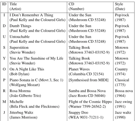
Table 1: Details of audio data used in experiments
Implementation and Results
Implementation Details
The beat tracking system is implemented on a Linux platform in C++, and consists of approximately 7000 lines of code in 18 classes. On a 500MHz Pentium computer, audio beat tracking takes under 20% of the length of the music (i.e. a 5 minute song takes less than one minute to process) and beat tracking of symbolic data is much faster, taking between 2% and 10% of the length of the music, depending on the note density.
Audio Data
The audio data used in these experiments is listed in Table 1, which also provides the letters used to identify the pieces in the text. The pieces were chosen to represent various styles of music, and are listed in order of subjective beat tracking difficulty.
The first 3 pieces (I,D,U) are standard modern pop/rock songs, characterised by a very steady tempo, which is clearly defined by simple and salient drum patterns, similar to the data used in the early audio beat tracking work of Goto and Muraoka (1995). In these songs the performed beat is very regular, with only small deviations from metrical
timing. It is assumed that this is the simplest type of data for beat tracking.
The next 2 pieces (S, Y) have a Motown/Soul style, characterised by more syn-copation, greater tempo fluctuations (5-10% in these examples), and more freedom to anticipate or lag behind the beat. It is expected that these examples are more difficult for a beat tracking system, but only of medium difficulty.
The remaining pieces were chosen as having particular characteristics which make beat tracking difficult. The Bob Dylan song (O) is made difficult by the fact that the drums are not prominent, and there is a much lower correlation between the beat and the events than in the other styles, due to his idiosyncratic style of singing and playing against the rhythmic context.
The classical piece (P), the first section of the third movement of Mozart’s Piano Sonata in C major (KV279), was synthesised from the MIDI data used in the beat tracking experiments using symbolic input data. This piece was chosen as an example of a piece with significant tempo fluctuations.
The next piece (R) is a live bossa nova performance with syncopated guitar and vocals, and very little percussion to indicate beat times. Sections of this piece are difficult for humans to beat track.
The two jazz pieces (M,J) were chosen for their particularly complex, syncopated rhythms, which are difficult even for musically trained people to follow. These pieces also provided examples of a different meter and swing eighth notes.
Tempo Induction Results
The tempo induction algorithm for audio data was tested on short segments of the above pieces to determine how reliably the ranked tempo hypotheses agreed with the measured tempo. (Piece P was not available at the time of this experiment.)
The tempo induction algorithm was applied to segments of 5, 10, 20 and 60 seconds duration of each piece, starting at each 1 second interval from the beginning of the piece. A tempo hypothesis was considered correct if the inter-beat interval was within 25ms of the measured inter-beat interval. Table 2 shows the results for 10 second excerpts, showing the position that the correct tempo hypothesis was ranked by the tempo induction algorithm. The results are presented as percentages of the total number of segments. The cumulative sums of rankings are shown in Figure 6.
Table 3 shows the effect of length of the segments on tempo induction. Each col-umn represents a different segment size, and the entries show the percentage of seg-ments for which the correct tempo was included in the top 10 ranked clusters. Even with 5 second segments, the tempo induction algorithm is quite reliable, and reliability increases with segment size.
The tempo induction stage provides a solid foundation for the beat tracking agents to work from, and is robust even for highly syncopated pieces of music. We now present the beat tracking results, first for audio data, and then the MIDI-based experi-ments.
ID Ranking of Correct Tempo Sum of 1 2 3 4 5 6 7 8 9 10 top 10 I 85.9 13.1 1.0 0.0 0.0 0.0 0.0 0.0 0.0 0.0 100.0 D 91.0 9.0 0.0 0.0 0.0 0.0 0.0 0.0 0.0 0.0 100.0 U 96.3 3.7 0.0 0.0 0.0 0.0 0.0 0.0 0.0 0.0 100.0 S 31.2 40.5 18.6 7.0 0.5 0.0 0.0 1.4 0.5 0.0 99.5 Y 86.7 11.7 0.8 0.0 0.0 0.0 0.0 0.0 0.0 0.0 99.2 O 83.9 12.9 2.4 0.0 0.0 0.8 0.0 0.0 0.0 0.0 100.0 R 58.7 18.2 7.6 3.6 1.3 2.7 0.9 0.9 0.0 0.9 94.7 M 16.9 25.9 16.9 12.9 4.7 6.5 1.8 1.8 1.8 1.1 90.3 J 61.5 13.4 9.2 3.1 4.2 0.4 0.4 0.4 0.0 0.0 92.4
Table 2: Beat induction of 10 second segments of songs. All figures are percentages of the total number of segments
1 2 3 4 5 6 7 8 9 10 10 20 30 40 50 60 70 80 90 100 Cluster ranking
Percentage of segments correct
M S R J O U D I,Y
Figure 6: Tempo induction results for 10 second segments shown as cumulative sums of percentages from Table 2
Piece Correct Tempo in Top 10 ID 5s 10s 20s 60s I 100.0 100.0 100.0 100.0 D 100.0 100.0 100.0 100.0 U 100.0 100.0 100.0 100.0 S 93.5 99.5 99.5 100.0 Y 96.9 99.2 100.0 100.0 O 95.2 100.0 100.0 100.0 R 84.9 94.7 100.0 100.0 M 84.9 90.3 95.3 95.9 J 79.2 92.4 97.6 99.1
Table 3: Effects of segment length on tempo induction: for each segment length, the percentage of segments with the correct tempo in the top 10 hypotheses is shown
ID Tempo range Meter Results I 139-142 4/4 100% D 151-154 4/4 100% U 145-146 4/4 100% S 96-104 4/4 96% Y 127-136 4/4 92% O 136-140 4/4 79% P 120-150 2/4 90% R 128-134 4/4 95% M 180-193 3/4 92% J 155-175 3/4 77%