Automatically Combining Static Malware Detection Techniques
David De Lille, Bart Coppens
Computer Systems Lab
Ghent University, Belgium
[email protected]
Daan Raman
NVISO CVBA, Belgium
[email protected]
Bjorn De Sutter
Computer Systems Lab
Ghent University, Belgium
[email protected]
Abstract
Malware detection techniques come in many different flavors, and cover different effectiveness and efficiency trade-offs. This paper evaluates a number of machine learn-ing techniques to combine multiple static Android malware detection techniques using automatically constructed deci-sion trees. We identify the best methods to construct the trees. We demonstrate that those trees classify sample apps better and faster than individual techniques alone.
1
Introduction
After having been a plague on mostly Windows-based computers for decades, malware is now also massively tar-geting Android-based devices. Consumers wanting to pro-tect themselves against Android malware can to some ex-tent rely on Google’s malware detection as applied to all apps in the Google Play Store, i.e., the official Android app store. However, no such automated detection exists for non-official stores such as the Chinese stores Baidu App Store and Tencent App Gem. Furthermore, even users that use only the Google Play Store might want to have a second opinion on whether an app contains malware or not. It is therefore not surprising that a lot of anti-virus companies such as AVG, AVAST, Kaspersky, McAfee, BitDefender, etc., all provide malware scanners on the Google Play An-droid Store, and that a lot of malware detection techniques have been published in scientific literature [1, 6, 7, 10, 14]. To scan apps en masse, scanners need to be fast. Yet they also have to be accurate, and higher accuracy most of-ten comes at the price of longer scanning times. As a result, the area of malware detection techniques is still very ac-tive. In turn, malware writers also deploy evolving detection evasion techniques. In this ever changing landscape, a re-curring problem is to decide which malware detection tech-niques to use. In terms of effectiveness, a scanner should deploy most if not all of the available techniques, but in terms of efficiency, that would be detrimental. So scanner
designers and users have to make a choice, based on a trade-off between effectiveness and efficiency. Apart from the raw effectiveness with which they classify samples into good-ware and malgood-ware and their efficiency in terms of running times, different malware detection techniques have differ-ent strengths, in the sense that they iddiffer-entify some types of malware better than others. Moreover, some detection tech-niques are easier to evade than others.
This paper assesses a range of machine learning (ML) methods to automate this decision problem. We focus on automated methods to build decision trees (DTs) in which each path consists of a specific sequence of existing mal-ware detection techniques. At every node, an existing scan-ning technique is applied to a sample, of which the outcome determines either the final classification of the sample as goodware or malware or the next technique to be applied.
Our design goals for generating the DTs are that they should be fast, and that they should be able to identify new kinds of malware. To keep the system fast, we include only static analysis techniques. In order to focus on detecting previously unknown malware variants, our system willnot
include any technique relying on fingerprints of known mal-ware. However, we do use techniques that try to detect un-known variants of un-known malware. Finally, we only im-plemented publicly known techniques that we were able to re-use as is, or that we could easily reimplement.
Our contributions are the the following:
1. We evaluate five methods to construct DTs of static malware detection techniques, and identify a clear winner to supporting a user or designer in trading off effectiveness vs. efficiency.
2. We compare the effectiveness of those DTs to the ef-fectiveness of a range of other supervised ML tech-niques that do not allow to trade off effectiveness for efficiency.
3. We demonstrate that combinations of detection tech-niques provide better and faster results than individual techniques alone.
4. We demonstrate that trivial heuristics that lack the re-quired accuracy to be used as stand-alone scanners, are in fact very useful when combined with existing tech-niques to minimize the average scanning time. 5. We propose adaptations to some existing techniques to
make them suitable for inclusion in DTs.
Section 2 describes background about DTs and ML. Next, Section 3 describes our experimental set-up, includ-ing the used data sets and detection algorithms. Section 4 then presents results, and Section 5 draws conclusions.
2
Decision Trees and Machine Learning
We want to combine existing malware detection tech-niques. Our ultimate goal is to have better classification than what is achievable by the individual techniques, at a lower cost than applying all techniques together. Specifi-cally, we want to use ML techniques to generate an opti-mized decision process that selects and applies a subset of the existing techniques in an order that optimizes both the efficiency, i.e, the computation time, and the effectiveness, i.e., the classification result, of the detection when applied to new samples.
For the classification decision process, we will use DTs, in which each leaf node corresponds to a final label with which a tested sample is labeled. In this paper, the samples are apps, and the labels are “malware” and “goodware”.
The internal (non-leaf) nodes of DTs model a flow-chart process, in which each node corresponds to an attribute be-ing evaluated and each branch represents the outcome of an evaluation. The paths from the root to the leafs represent the decision process, which in this case corresponds to the set of classification rules. In the context of this paper, the sample attributes evaluated in the internal nodes are the samples’ classification into goodware or malware by the existing, in-dividual malware detection techniques. Each sample evalu-ation in an internal node has an associated cost: the compu-tation time required by the malware detection technique to analyze the app. Both the efficiency and the effectiveness of a DT hence depend on its internal structure, i.e., on how the existing techniques are combined.
To generate an optimal DT structure with which we can classify new samples efficiently and effectively, we evalu-ated multiple ML approaches based on supervised learning. These approaches start from a so-called training set of sam-ples that are already labeled and of which all attributes are already computed. In other words, in our context they will start from a set of apps labeled as goodware or malware, and to which all the existing techniques have been applied during the so-called data collection phase of the approach.
In the training phase, the DT is then constructed based on the collected data. Initially, one attribute is chosen for
the whole training data set, using some metric. The train-ing set is then partitioned into subsets based on the value of this attribute. On each subset, the same partitioning al-gorithm is then applied recursively, obviously considering other attributes for each sub step.
The algorithm stops when all the samples in a subset be-long to the same class, in which case the subset as a whole can be labeled accordingly. Alternatively, the iterative parti-tioning into subsets stops when all the samples in a set have identical values for all attributes. In that case, the set of considered attributes has proven to be inconclusive. Such a final subset is then assigned the class label that occurs most often among the samples in the subset. This serves the goal of minimizing the number of incorrect classifications fol-lowing from the inconclusiveness.
The approaches proposed in literature and evaluated in our research differ in the metric they use for choosing an attribute for each partitioning step. For example, the most popular DT algorithm is called ID3 [15]. The selected at-tribute for each partition is chosen to be the atat-tribute that contributes the most information about the class when it is examined. It does so by calculating theinformation gainfor each attribute, which is based on the concept of entropy:
Frequency of classyin data setT :p(y) =|(T|y)|
|T|
Entropy of data setT :H(T) =−X y∈Y
p(y)·log2(p(y))
Subset after choosing attributeA:T = [
s∈S s Information Gain:IG(A, T) =H(T)−X s∈S H(s)· |s| |T|
Other metrics for generating DTs sometimes include a cost for using an attribute. With this cost, we can make a trade-off between the information gain and the cost of eval-uating an attribute. The alternative proposals from literature as listed below differ in how they combine information gain and cost into a metric for choosing the best attribute:
ID3 [15]:information gain
EG2 [13]:(2(information gain)−1)/(attribute cost+ 1)ω CS-ID3 [17]:(information gain)2/attribute cost
IDX [12]:information gain/attribute cost
CSGain [5]:(Na/N)·information gain−ω·attribute cost
The parameter ω, used for EG2 and CSGain, can be ad-justed by the user to indicate the relative importance of in-formation gain and cost. Nis the amount of samples in the entire training set andNa is the amount of samples in the
current data set for which an attribute has to be selected. Moreover, to avoid that the learning approach overfits the DT onto the training set, we imposed two additional
conditions before a data set is partitioned: first of all, the number of samples in the data set has to be high enough, and secondly, a dataset can not be partitioned if the in-formation gain of the chosen attribute is too small. DTs are only one form of classification techniques that can be trained using supervised learning methods. We also eval-uated some other techniques. In particular, these are k -nearest neighbor (NN) [4], naive Bayesian networks [9], neural networks [16], support vector machines [3] and lin-ear discriminant analysis [11], all of which are readily avail-able in the ML software package RapidMiner Studio v6.
These additional techniques do not consider cost metrics. This is the case because for classifying a new sample app as malware or goodware once the training has been finalized, these techniques first require the deployment of allof the individual detection techniques on the app, whereas the DT approach will only have to apply the techniques on the path followed during the classification process.
3
Experimental Setup
This section discusses the data collection and the mal-ware detection techniques that the ML algorithms will use as input. Seven techniques are taken from literature, and we designed three basic additional techniques. Both our adap-tations to the existing techniques, and our additional heuris-tics are discussed, as is our experimental methodology.
3.1
Data Set
The training data set for this study consists of 1858 An-droid goodware apps and 1598 AnAn-droid malware apps. The goodware samples were collected from the top 60 apps in each of the 34 categories of the Google Play store using a service called APK Downloader. We collected the malware samples from two different sources: from the Android Mal-ware Genome Project [19], and from the Contagio Mobile blog. We excluded 39 samples from our original data set for two reasons. First, we excluded some samples because they could not be handled by all the detection tools we re-ceived from their authors. Secondly, we excluded some sup-posed malware samples because the VirusTotal online mal-ware scanner did not classify them as malmal-ware.
For validation purposes, it is important to establish a cor-rect ground truth, i.e., the corcor-rect label is assigned to each sample app. This is not a problem for the malware samples, because these apps have already been confirmed to contain malicious code by malware analysts. In theory it is possible, however, for our goodware apps to also contain malware. In practice, this is highly unlikely for two reasons. First, as these apps were in the top-60 of a certain app category, they have been downloaded and tested by a lot of people. Secondly, the Google Play store makes use of the Google
Bouncer service that scans all apps for malware and applies dynamic malware detection techniques.
3.2
Existing Detection Techniques
For our research, we selected existing techniques of which we could receive implementations from their authors or about which enough documentation was available to re-implement the technique confidently. Furthermore, we con-sidered the orthogonality of the approaches with respect to the types of features they use for their classification.
Adagio Adagio uses a predictive model based on Support Vector Machines [10]. To build the training data, Adagio first constructs the call graph (CG) of each app. Every node in the CG represents a procedure and gets assigned a hash value that describes the properties of the procedure’s neigh-bors in the CG. Then the number of times each hash value is present in the graph is counted. These values are trans-formed into a vector that characterizes the app.
The vectors of the training set are used to create a predic-tive model to classify new apps. Gascon et al. report a pre-cision of 89% and a false positive rate of 10% for this tech-nique as applied on 135792 goodware samples and 12158 malware samples [10]. We obtained the Python implemen-tation of this technique from them.
API-1NN Based on DroidAPIMiner by Aafer et al., API-1NN is a nearest neighbor approach that classifies apps based on the API calls detected in them [1]. For training, the signatures of called methods in the Android API are ex-tracted from the apps. The original DroidAPIMiner num-bers all those API calls. A bit vector then represents which API calls are present in a sample. After training, a simi-lar bit vector is computed on a new app to classify, and the nearest neighbor approach is applied to this bit vector.
We did not obtain the original implementation by the original authors, and hence had to re-implement it. More-over, since one of our requirements is that the creation of DTs can be redone in an evolving landscape of malware techniques and anti-malware techniques, we cannot assume the existence of one fixed mapping of API calls to numbers. Therefore we adapted the method as follows: Each API call is then hashed and the remainder of this hash value mod
N, with a given integerN, is computed. A bit vector of size N is then constructed, in which each bit in positionn, with0≤n < N, indicates whether or not an API that was hashed into the valuenwas present in the app.
For our own implementation, we experimentally deter-mined the appropriate value for N to be 1500. Whereas the original authors reported a precision of 99% for their technique, our re-implementation was only able to achieve 95.5%. This might be due to the different training set, or because of undocumented details of the original implemen-tation that we could not re-implement.
Risk Scoring Schemes Peng et al. described four related techniques that try to quantify theriskof Android apps [14]. Rather than presenting the user with a set of permissions re-quested by an app, they propose a single risk score, that indicates to users the risk involved in installing and using the app. They use probabilistic generative models based on naive Bayes classifiers. As attributes, they consider the cat-egory of an app, and the permissions the app requests in its so-called manifest, the idea being that permissions re-quested by one app, but not typically rere-quested in its cate-gory, makes an app suspicious. In order of increasing com-plexity, the proposed variations proposed by Peng et al. are: 1. Basic Naive Bayes (BNB) only considers permissions. 2. Naive Bayes with Informative Priors (PNB) in addition builds on the a priori knowledge that some permissions are more dangerous than others.
3. Mixture Naive Bayes with Categories (MNBC) con-siders the category of an app, besides its permissions; 4. Hierarchical Mixture of Naive Bayes (HMNB)
consid-ers a uniform partitioning of categories into subclasses. All four variations performed more or less equally well, with HMNB performing slightly better. We obtained a C++ implementation from the original authors, who reported that the MNBC implementation was problematic. We thus did not use that variation in our experiments.
It is important to note that unlike the previous tech-niques, these risk scoring schemes do not assign class labels (goodware or malware). Instead, the produced risk scores are numbers that indicate how dangerous the app might be. These scores are converted to the desired binary class output using a threshold. The optimal threshold was determined by first calculating the risk scores of the training samples and finding the threshold that best classified these samples.
DroidLegacy DroidLegacy is a technique introduced by Deshotels et al. It is designed to detect repackaged mal-ware [6]. This is a type of malmal-ware that is created by taking a goodware app and adding malicious code to it. When two apps contain very similar malicious code, they are said to belong to the same malware family.
This technique groups the classes of an app into mod-ules that are characterized by their API calls. By comparing training samples of the same malware family, the recurring malicious module can be identified and this will act as a signature for the malware family. Then, every test sample is compared to every signature and a value between 0 and 1 in-dicates how well the sample fits the signature. The score is then converted to a class prediction using a threshold, simi-lar to the Risk Scoring schemes.
The original authors gave us access to their source code, which required little adaptations for our experimental setup. However, we did discover that in our training set, a lot of
false positive results were reported, due to some used sig-natures being too generic, and hence spanning significantly more than a single malware family. To improve the per-formance of this technique, we manually searched for the signatures causing the false positives, and excluded them.
Kirin Kirin is one of the oldest techniques for detecting Android malware [7]. Its goal is to inform a user when cer-tain dangerous combinations of permissions are requested by an app. Kirin has seven combinations of permissions that are not allowed. If one of these seven rules is triggered, the sample is considered to be malicious.
While the original code of Kirin is available, we reim-plemented it: the original code is designed to prompt a user of an Android device on installing an app, whereas we want our detection techniques to run on a non-Android server.
3.3
Additional Detection Heuristics
In addition to reusing the aforementioned existing tech-niques, we developed three new heuristics. These new heuristics primarily focus on efficient ways to identify highly likely goodware and highly likely malware, albeit at the cost of many false negatives. As we only intent to com-bine the heuristics with other techniques, their high false rates are not necessarily problematic.
Permissions Decision Tree Our first heuristic uses a DT to classify goodware and malware based on the permissions requested by an app. In addition to this extremely sim-ple classification, we created an additional Permissions-DT-Enhanced technique, that in addition to the app’s permis-sions also takes into account the invocation or incorporation of encryption APIs, dynamic loading, reflection, and native code. We generate the DT based on the training data.
Contains APK In addition to the above permission DTs, we include a simple check for whether or not the Android application package (APK), contains another APK file it-self. We did so because there are certain malware apps that don’t appear to be dangerous at all, but that do have an APK file embedded in them that contains the malicious code. By itself, this technique has a very low accuracy (only 64.92%), but it has a very strong positive predictive value (95.48%), which is higher than that of all the existing techniques, and it has an extremely low cost. That is why we added it to our suite of possible detection “techniques”.
Has Permissions Our final heuristic checks whether an app happens to request no permissions at all. As soon as an app requests a permission, the predicted class will be malware. This provides an extremely fast way to conclude that an app probably is goodware. After all, an app with no permissions is extremely limited in what it can abuse.
3.4
Methodology
By means ofk-fold cross-validation, we can prevent the ML algorithms from over-fitting the malware samples in the data set, while at the same time still making use ofallthe malware samples in the data set to train and evaluate our framework [2]. With this technique, the data set is ran-domly partitioned inksets. In each ofkexperiments, one of these sets is used as a validation set, while the otherk−1 sets are used as training inputs for the ML algorithms. In other words, we repeat the experiments of constructing a DTktimes, and evaluate each DT on a validation data set of which no samples were used for the DT’s construction. We chose to use 10-fold, and report the average cost and accuracy of the 10 evaluations.
Some of the individual detection techniques first also need to be trained by means of data sets. To train those techniques on each of the training sets for the global 10-fold cross-validation, we used 3-fold cross-validation.
We already mentioned in Section 2 that there are two pa-rameters to consider for generating a DT: the minimal num-ber of samples in a data set before that set can be split, and the minimal information gain for an attribute of a data set before that data set can be split. In addition, some DT al-gorithms have an additional parameterω. This parametriza-tion allows us to generate many different DTs using each of the evaluated ML algorithm, with each DT being char-acterized by its efficiency (i.e., cost) in terms of average execution time, and by its effectiveness in term of achieved classification accuracy. As each of the evaluated algorithms are fast enough to generate thousands of DTs per minute (given our data set sizes), we performed a parameter sweep, and report the cost/accuracy Pareto front.
All our measurements were executed on an 32-bit Intel Core 2 Duo system clocked at 2GHz, with 6GiB of RAM. To speed up our ML experiments, we evaluated all tech-niques once on each app, recording the results and execu-tion time of the analysis. The average execuexecu-tion time of the technique is used as the cost for generating the DTs. The execution time of a generated DT is then the average time required to analyze an app from the validation set.
We evaluate and rank the different algorithms based on standard metrics for evaluating binary classifications [8, 18]. These metrics assess how well the labels assigned to the samples by a DT match the ground truth. A sam-ple that is correctly identified as malware is a True Posi-tive (T P), a sample that is correctly identified as goodware is a True Negative (T N). A malware sample that is mis-identified as goodware is a False Negative (F N), whereas goodware that is mis-identified as malware is a False Posi-tive (F P). Thesensitivityis defined asT P/(T P +F N), and is a measure for how well the classification correctly identifies malware. ThespecificityisT N/(T N+F P), and
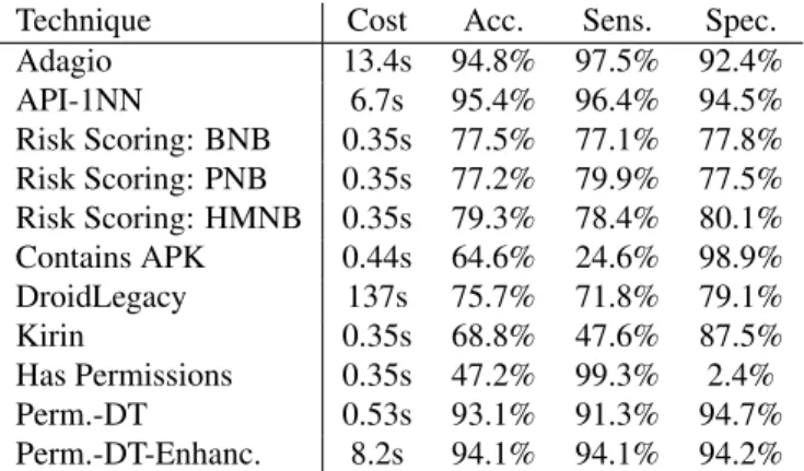
Technique Cost Acc. Sens. Spec. Adagio 13.4s 94.8% 97.5% 92.4% API-1NN 6.7s 95.4% 96.4% 94.5% Risk Scoring: BNB 0.35s 77.5% 77.1% 77.8% Risk Scoring: PNB 0.35s 77.2% 79.9% 77.5% Risk Scoring: HMNB 0.35s 79.3% 78.4% 80.1% Contains APK 0.44s 64.6% 24.6% 98.9% DroidLegacy 137s 75.7% 71.8% 79.1% Kirin 0.35s 68.8% 47.6% 87.5% Has Permissions 0.35s 47.2% 99.3% 2.4% Perm.-DT 0.53s 93.1% 91.3% 94.7% Perm.-DT-Enhanc. 8.2s 94.1% 94.1% 94.2%
Table 1. Results of the individual techniques
is a measure for how well the classification correctly iden-tifies goodware. Finally, these measures can be combined into a single measure called theaccuracy, which is defined as(T P +T N)/(T P+F N+T N+F P).
4
Results
We start by investigating the results of the individual de-tection techniques. Table 1 shows the aggregated results. The first thing to note is the vast range of execution time per technique: the fastest techniques take less only about 1/3 of second. These are the techniques that essentially only open the APK file to inspect the permissions, such as theKirin
andHas Permissionstechniques. At the opposite end are the techniques that require extraction of significantly more information from the APK, such as the used API calls in the case ofAPI-1NN, and information about the call graphs in the case ofAdagio.
Furthermore, note that the slow techniques do not neces-sarily perform better than the faster techniques on our data set. For example, while DroidLegacy is the slowest tech-nique, it has a lower accuracy than many of the techniques that take less than a second to execute. However, in this class of techniques that on average take less than a second to execute, there is still significant variation in the accuracy. For example, the simpleHas Permissions check performs significantly worse thanKirin, even though both techniques are equally fast. However, note that theHas Permissions
check is especially good at correctly identifying goodware, as can be seen from its sensitivity of over 99%.
Next, we investigated combining these individual tech-niques by using DTs. Figure 1 shows the Pareto fronts of the different DT construction algorithms. Please note that per parameter setting, 10 DTs are generated for the 10 cross-validation experiments. Points on the Pareto fronts repre-sent average costs and accuracies over those 10 DTs. Given the high accuracy of fast techniques such as Permissions
0.93 0.94 0.95 0.96 0.97 0.98 Accuracy 0 10 20 30 40 50 60 Cost (in s) ID3 EG2 CSID3 IDX CSGain Figure 2 Figure 3
Figure 1. Pareto fronts of cost vs. accuracy of DTs generated with different strategies.
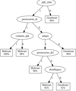
API_1NN permissions_dt 1 Goodware 96% 0 contains_apk 1 adagio 0 Malware 100% 1 Malware 98% 0 permissions_dt2 1 Goodware 90% 0 Malware 90% 1 droidlegacy 0 Malware 92% 1 Goodware 52% 0
Figure 2. DT with an accuracy of 97.0% and an average execution time of 16.1s.
DT, the graph only show results for DTs that deliver an av-erage accuracy of more than 93%.
Irrespective of the trade-off that one wants to make be-tween cost and accuracy, the EG2 strategy consistently de-livers the best DTs. Only when the fastest DTs are consid-ered, at the cost of significantly lower accuracy, do the DTs generated using the IDX algorithm come close to the per-formance of EG2-generated DTs. This consistent result of EG2 is somewhat surprising, as in other domains such as
forensics classification, more recent algorithms parametriz-able with the sameωperformed much better.
Another interesting result is that the choice of algorithm significantly influences the average analysis time. For ex-ample, DTs built with EG2 can achieve an accuracy of at least 97% with an average analysis time of less than 20 sec-onds, whereas using the CSGain algorithm results in DTs that on average require more than 50 seconds to get the same accuracy. So EG2 not only consistently delivers better DTs, it delivers much better ones.
Whereas the best performance of the individual tech-niques is 95.3%, using DTs we can achieve a performance of 97.6%, with an execution time of only 61 seconds. In practice, however, we would choose the DTs generated with EG2 that achieve slightly less than 97.5%, but have an exe-cution time of less than 30 seconds, which still have a sig-nificantly higher accuracy than the individual techniques.
The simplest DTs correspond to running a single detec-tion technique and presenting that result to the user. For instance, the DT with an accuracy of 93.1% corresponds to a single check of thePermissions DT analysis. More inter-esting behavior shows up once the DTs combine different analysis techniques. Figure 2 shows one of the DTs gener-ated using the EG2 algorithm that correspond to the Pareto-optimal point with an accuracy of of 97.0% and an average execution time of 16.1 seconds. This point is labeled in the Pareto curves of Figure 1. Because we use 10-fold cross-validation, this is only one out of 10 generated DTs for that Pareto point. In each leaf node of the DT, the label given to a simple is depicted, as well as theconfidencethat the label is correct. This confidence equals the number of all train-ing samples that were labeled correctly by the leaf node, divided by the total number of samples labeled by it.
We see that a single negative check of theAPI-1NN tech-nique is sufficient to classify a sample as malware. How-ever, to improve the accuracy, the DT tries to minimize the impact ofAPI-1NN’s false positives by running more anal-yses whenAPI-1NNsuggests that the sample is malware.
Note that this automatically generated DT can still be im-proved (manually) when the user is only interested in the fi-nal classification, but not in the confidence of it: Regardless of the result of theContains APK test, the produced label isMalware. In other words, even though the test requires some execution time, it has no impact on the classification whatsoever. So we could simply remove it to obtain an even faster DT, with the same accuracy.
This test was included in the DT is because of the lack of lookahead in the greedy EG2 construction algorithms: WhileContains APKwas the best technique to split the data set at some point during the iterative construction of the DT, the chosen parameters prevented the remaining sets from being split further. As both sets contain more malware than goodware, both are labeled as malware.
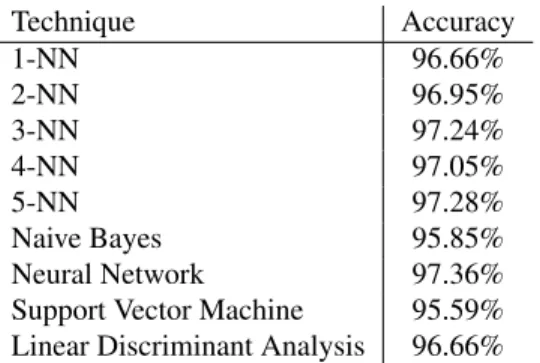
Technique Accuracy 1-NN 96.66% 2-NN 96.95% 3-NN 97.24% 4-NN 97.05% 5-NN 97.28% Naive Bayes 95.85% Neural Network 97.36% Support Vector Machine 95.59% Linear Discriminant Analysis 96.66% Table 2. Results of the other ML techniques
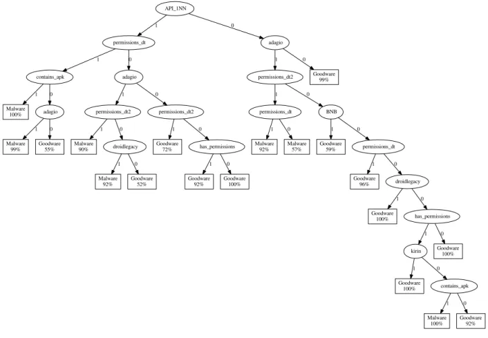
To achieve more accurate decisions, more complex DTs need to be generated. Figure 3 shows one of the DTs for an accuracy of 97.4% and an average execution time of 26.5 seconds. Again, this point is labeled in the Pareto curves of Figure 1. The top part of this DT is relatively balanced in the number of techniques that need to be applied for each sam-ple. Only the bottom right stands out with a rather narrow subtree, of which only a single leaf node represents mal-ware. This subtree furthermore includes a decision based onDroidLegacy, the slowest individual technique. In this case, the advantages of DTs are obvious: Even though it is by far the slowest malware detection technique, it is still useful in this case because not only can it usefully contribute to an accurate classification, the induced average overhead is relatively small, due to the fact that this subtree contains only 5% of the samples.
Table 2 shows the accuracies obtained with alternative ML techniques. For the parameterizable techniques, we chose the default values as they are set in the RapidMiner ML framework. Do note that, because these algorithms do not take into account the cost and because they require all of the individual detection techniques to be deployed on a sample in order to classify the sample, the average execu-tion time of all of these techniques is the sum of the average times ofallindividual detection techniques, which is about 170 seconds in our setup. Even though the DTs use only a subset of the detection techniques to base their classification on, they clearly outperform the other ML techniques.
Because of our use of only default parameters, it is possi-ble that a different combination of parameters would allow these alternative classification techniques to get a higher ac-curacy. Even so, the total analysis time per sample would still be more than 6 times higher than that of the DT shown in Figure 3.
5
Conclusions
We have demonstrated that DTs provide an excellent strategy to combine different static malware detection tech-niques into a single framework that is optimized for both
a high classification accuracy, while keeping the analysis time low. In particular, we have shown that by using the EG2 algorithm to construct the decision trees, malware can be classified significantly better than could be done using the individual detection techniques, without needing to pay the overhead of executing all detection techniques. Further-more, we show that these DTs can outperform other ma-chine learning techniques that combineallindividual mal-ware detection techniques.
References
[1] AAFER, Y., DU, W.,ANDYIN, H. DroidAPIMiner: Mining API-level features for robust malware detec-tion in Android. InSecurity and Privacy in Commu-nication Networks, vol. 127 ofLecture Notes of the Institute for Computer Sciences, Social Informatics and Telecommunications Engineering. Springer Inter-national Publishing, 2013, pp. 86–103.
[2] BISHOP, C. M. Pattern Recognition and Machine Learning. Springer, 2006.
[3] CORTES, C., AND VAPNIK, V. Support-vector net-works.Machine learning 20, 3 (1995), 273–297. [4] COVER, T., AND HART, P. Nearest neighbor
pat-tern classification. IEEE Trans. Inf. Theor. 13, 1 (Jan. 1967), 21–27.
[5] DAVIS, J., HA, J., ROSSBACH, C., RAMADAN, H., ANDWITCHEL, E. Cost-sensitive decision tree learn-ing for forensic classification. InMachine Learning: ECML 2006, vol. 4212 ofLecture Notes in Computer Science. Springer Berlin Heidelberg, 2006, pp. 622– 629.
[6] DESHOTELS, L., NOTANI, V., AND LAKHOTIA, A. Droidlegacy: Automated familial classification of An-droid malware. In Proc. of ACM SIGPLAN Pro-gram Protection and Reverse Engineering Workshop (PPREW)(2014), pp. 3:1–3:12.
[7] ENCK, W., ONGTANG, M.,ANDMCDANIEL, P. On lightweight mobile phone application certification. In
Proc. 16th ACM Conf. on Computer and Communica-tions Security (CCS)(2009), pp. 235–245.
[8] FAWCETT, T. An introduction to ROC analysis. Pat-tern Recognition Letters 27, 8 (June 2006), 861–874. [9] FRIEDMAN, N., AND GOLDSZMIDT, M. Building
classifiers using bayesian networks. InProc. 13th Na-tional Conf. on Artificial Intelligence (AAAI)(1996), pp. 1277–1284.
API_1NN permissions_dt 1 adagio 0 contains_apk 1 adagio 0 Malware 100% 1 adagio 0 Malware 99% 1 Goodware 55% 0 permissions_dt2 1 permissions_dt2 0 Malware 90% 1 droidlegacy 0 Malware 92% 1 Goodware 52% 0 Goodware 72% 1 has_permissions 0 Goodware 92% 1 Goodware 100% 0 permissions_dt2 1 Goodware 99% 0 permissions_dt 1 BNB 0 Malware 92% 1 Malware 57% 0 Goodware 59% 1 permissions_dt 0 Goodware 96% 1 droidlegacy 0 Goodware 100% 1 has_permissions 0 kirin 1 Goodware 100% 0 Goodware 100% 1 contains_apk 0 Malware 100% 1 Goodware 92% 0
Figure 3. DT with an accuracy of 97.4% and an average execution time of 26.5s.
[10] GASCON, H., YAMAGUCHI, F., ARP, D., AND RIECK, K. Structural detection of Android malware using embedded call graphs. InProc. ACM Workshop on Artificial Intelligence and Security (AISec)(2013), pp. 45–54.
[11] LACHENBRUCH, P. A. Discriminant analysis. Wiley Online Library, 1975.
[12] NORTON, S. W. Generating better decision trees. In
Proc. 11th Int’l Joint Conf. on Artificial Intelligence (IJCAI)(1989), pp. 800–805.
[13] NEZ, M. The use of background knowledge in de-cision tree induction. Machine Learning 6, 3 (1991), 231–250.
[14] PENG, H., GATES, C., SARMA, B., LI, N., QI, Y., POTHARAJU, R., NITA-ROTARU, C.,ANDMOLLOY, I. Using probabilistic generative models for ranking risks of Android apps. InProc. ACM Conf. on Com-puter and Communications Security (CCS) (2012), pp. 241–252.
[15] QUINLAN, J. Induction of decision trees. Machine Learning 1, 1 (1986), 81–106.
[16] RUMELHART, D. E., HINTON, G. E., AND WILLIAMS, R. J. Neurocomputing: Foundations of Research. MIT Press, 1988, ch. Learning Representa-tions by Back-propagating Errors, pp. 696–699. [17] TAN, M. Cost-sensitive learning of classification
knowledge and its applications in robotics. Machine Learning 13, 1 (1993), 7–33.
[18] WITTEN, I. H., FRANK, E.,ANDHALL, M. A.Data Mining: Practical Machine Learning Tools and Tech-niques, third ed. Morgan Kaufmann, 2011.
[19] ZHOU, Y., AND JIANG, X. Dissecting android mal-ware: Characterization and evolution. InIEEE Symp. on Security and Privacy (S&P)(2012), pp. 95–109.