Theses 12-2020
Scalable Real-Time Rendering for Extremely Complex 3D
Scalable Real-Time Rendering for Extremely Complex 3D
Environments Using Multiple GPUs
Environments Using Multiple GPUs
Yangzi DongFollow this and additional works at: https://scholarworks.rit.edu/theses
Recommended Citation Recommended Citation
Dong, Yangzi, "Scalable Real-Time Rendering for Extremely Complex 3D Environments Using Multiple GPUs" (2020). Thesis. Rochester Institute of Technology. Accessed from
This Dissertation is brought to you for free and open access by RIT Scholar Works. It has been accepted for inclusion in Theses by an authorized administrator of RIT Scholar Works. For more information, please contact
by
Yangzi Dong
A dissertation submitted in partial fulfillment of the requirements for the degree of
Doctor of Philosophy
in Computing and Information Sciences
B. Thomas Golisano College of Computing and Information Sciences
Rochester Institute of Technology Rochester, New York
by Yangzi Dong
Committee Approval:
We, the undersigned committee members, certify that we have advised and/or supervised the candidate on the work described in this dissertation. We further certify that we have reviewed the dissertation manuscript and approve it in partial fulfillment of the requirements of the degree of Doctor of Philosophy in Computing and Information Sciences.
Dr. Chao Peng Date
Dissertation Advisor
Dr. Joe Geigel Date
Dissertation Committee Member
Dr. Christopher Egert Date
Dissertation Committee Member
Dr. Yunbo Zhang Date
Dissertation Committee Member
Dr. David Long Date
Dissertation Defense Chairperson Certified by:
Dr. Pengcheng Shi Date
Ph.D. Program Director, Computing and Information Sciences
©2020, Yangzi Dong All rights reserved.
Yangzi Dong Submitted to the
B. Thomas Golisano College of Computing and Information Sciences Ph.D. Program in Computing and Information Sciences
in partial fulfillment of the requirements for the
Doctor of Philosophy Degree
at the Rochester Institute of Technology
Abstract
In 3D visualization, real-time rendering of high-quality meshes in complex 3D environments is still one of the major challenges in computer graphics. New data acquisition techniques like 3D mod-eling and scanning have drastically increased the requirement for more complex models and the demand for higher display resolutions in recent years. Most of the existing acceleration techniques using a single GPU for rendering suffer from the limited GPU memory budget, the time-consuming sequential executions, and the finite display resolution. Recently, people have started building com-modity workstations with multiple GPUs and multiple displays. As a result, more GPU memory is available across a distributed cluster of GPUs, more computational power is provided throughout the combination of multiple GPUs, and a higher display resolution can be achieved by connecting each GPU to a display monitor (resulting in a tiled large display configuration). However, us-ing a multi-GPU workstation may not always give the desired renderus-ing performance due to the imbalanced rendering workloads among GPUs and overheads caused by inter-GPU communication. In this dissertation, I contribute a multi-GPU multi-display parallel rendering approach for complex 3D environments. The approach has the capability to support a high-performance and high-quality rendering of static and dynamic 3D environments. A novel parallel load balancing algorithm is developed based on a screen partitioning strategy to dynamically balance the number of vertices and triangles rendered by each GPU. The overhead of inter-GPU communication is minimized by transferring only a small amount of image pixels rather than chunks of 3D primitives with a novel frame exchanging algorithm. The state-of-the-art parallel mesh simplification and GPU out-of-core techniques are integrated into the multi-GPU multi-display system to accelerate the rendering process.
assistance, encouragement and patience throughout my Ph.D. study. His guidance helped me in all the time of the research and in the successful completion of my dissertation. I would never forget the insightful conversations we have had on every imaginable topic and the opportunities he offered me on many interesting works and projects.
Besides, I would like to thank my dissertation committee members: Dr. Joe Geigel, Dr. Christopher Egert, Dr. Yunbo Zhang, for their interests, encouragement, valuable suggestions, and insightful comments. I would like to thank my dissertation chairperson: Dr. David Long for his kind assistance in serving as my Ph.D. defense chair. I also want to thank the Ph.D. program director, Dr. Pengcheng Shi for his great support.
I gratefully acknowledge the National Science Foundation Grant for the support and funding of the work presented in this dissertation.
Thanks to the support of MAGIC Center, the department of IGM and the Department of Com-puting and Information Sciences Ph.D. for providing me the workspace and research resources. I would like to thank all my dear friends for the pleasant moments of their accompany. Their help was much worth than I can express on paper. I would also like to give special thanks to my roommate and friend, Lizhou Cao, for his thoughtful suggestions and for always being available. I could not imagine I can reach this stage of my life without their support.
Last but not least, I would like to thank my parents for their unconditional love, continuous support, and everything they have done for me. I also would like to thank my loving wife, Dan Zhou, for giving me all the support, encouragement and patience. Thank you for always being by my side. To my families who were often in my thoughts on this journey — you are missed.
1 Introduction 1
1.1 Motivation . . . 2
1.2 Challenges in Multi-GPU . . . 5
1.3 Contribution . . . 7
1.4 Organization . . . 8
2 Multi-GPU Rendering Tools and Methods 10 2.1 Solutions with Distributed Clusters or Supercomputers . . . 10
2.2 Hardware Solutions . . . 11
2.3 Middleware Solutions . . . 13
2.4 Software Solutions . . . 15
2.4.1 Sort First Rendering . . . 16
2.4.2 Sort Middle Rendering . . . 18
2.4.3 Sort Last Rendering . . . 19
3 Screen Partitioning Load Balancing Algorithm 21 3.1 Dynamic Load Balancing . . . 21
3.1.1 Screen and Frustum Strips . . . 22
3.1.2 Load Balancing Algorithm and Parallelization . . . 22
3.2 Frame Exchanging between GPUs . . . 27
3.3 System Overview . . . 30
3.4 Multi-GPU Configuration . . . 31
3.5 Communication and Synchronization . . . 34
3.5.1 Camera Synchronization . . . 35
3.5.2 Rendering Synchronization . . . 35
3.5.3 Display Synchronization . . . 35
3.6 Evaluation . . . 36
3.6.1 Performance . . . 36
4 Multi-GPU Multi-Display Rendering System 41 4.1 GPU Acceleration Fundamentals . . . 41
4.1.1 Parallel Mesh Simplification . . . 42
4.1.2 Level of Detail Selection . . . 43
4.1.3 GPU Out-of-Core . . . 46
4.2 Half-Edge Collapsing for Data Preprocessing . . . 48
4.3 Overview of the Multi-GPU Multi-Display Rendering System . . . 49
4.3.1 GPU Tree . . . 49
4.3.2 Preprocessing and Data Management. . . 50
4.4 Execution Components of the System . . . 51 4.4.1 LOD Selection . . . 51 4.4.2 Load Balancing . . . 51 4.4.3 GPU Out-of-Core . . . 53 4.4.4 Mesh Reformation . . . 55 4.4.5 Rasterization . . . 56 4.4.6 Frame Exchanging . . . 56 4.4.7 Synchronization . . . 57 4.4.8 Display . . . 58 4.5 Evaluations . . . 58 4.5.1 Overall . . . 62 4.5.2 Performance Breakdowns . . . 62
4.5.3 Frame-by-Frame Performance Comparison . . . 64
4.5.4 Efficiency Comparison . . . 67
4.5.5 Comparison with the Equalizer . . . 71
4.5.6 Quality Comparison . . . 73
5 Large Dynamic Crowd Rendering on GPU 74 5.1 Related work in Crowd Rendering . . . 75
5.2 Crowd Rendering System Overview . . . 78
5.3 Fundamentals of LOD Selection and Character Animation . . . 80
5.3.2 Animation . . . 82
5.4 Source Character and Instance Management . . . 83
5.4.1 Packing Skeleton, Animation, and Skinning Weights into Textures . . . 84
5.4.2 UV-Guided Mesh Rebuilding . . . 85
5.4.3 Source Character and Instance Indexing . . . 87
5.5 Experiment and Analysis . . . 90
5.5.1 Visual Fidelity and Performance Evaluations . . . 91
5.5.2 Comparison and Discussion . . . 94
5.6 Efficiency of Multi-GPU Crowd Rendering . . . 96
6 Conclusion and Future Works 100 6.1 Conclusion . . . 100
6.2 Future work . . . 101
6.2.1 Parallel Load Balancing Algorithm in Cluster Rendering System . . . 101
6.2.2 Suitable Space Structure for GPU Out-of-Core Acceleration Technique . . . 101
1.1 The performance comparison between traditional rendering and visibility culling methods. [81] . . . 3 1.2 Examples of complex 3D models. (a) is an array of 20 duplicated UNC Power Plant
model composed of approximately over 120 million vertices and 254 million triangles organized in over 3 million objects. (b) is a large crowd rendering composed of 30,000 animated characters containing over 100 million triangles. . . 4
2.1 The example of two rendering modes in SLI. (a) is the Alternate Frame Rendering (AFR) mode. (b) is the Split Frame Rendering (SFR) mode. . . 12 2.2 Illustration of Equalizer. (a) is an example of Equalizer application. (b) is an
example of an execution flow for Equalizer applications. . . 14 2.3 The three sorting categories in parallel rendering described in [111]. (a) is the
sort-first approach, (b) is the sort-middle approach, (c) is the sort-last approach. . . 16 2.4 The example of software solution implemented by Equalizer [38]. (a) is an example of
sort-first approach implemented using 2D Compound in Equalizer. (b) is an example of sort-last approach implemented using DB Compound in Equalizer. . . 17
3.1 Four frustum strips generated by evenly partitioning the screen into four regions. The red rectangle on the near plane is the bounding rectangle of the projected object’s bounding volume. . . 23
3.2 An example of the load balancing algorithm for a non-leaf node in the GPU tree. A total of 10 objects are projected on the screen. ThestripN umis set to 16. Assume that the number of GPUs in two child nodes of this non-leaf node is same , so that the value ofbalRatiois equal to 1.0. . . 24 3.3 An example of identifying the GP U2’s screen region that it should render. There
are a total of eight GPUs. GPUs and their display monitors are configured with the column-major order. They are grouped into a binary search tree that has three tree node levels (log28 = 3), as the GPU tree shown in the left image. In the right image, the red screen region will be rendered by GP U2. (a) is the vertical partitioning line
with the ratio to partition the full screen. The first-level node thatGP U2 belongs to
obtains the screen region of [(0,0),(x(a), height)]. (b) is the vertical partitioning line
with the ratio to partition the screen region generated from (a). The second-level node that GP U2 belongs to obtains the screen region of [(x(b),0), (x(a), height)].
(c) is the horizontal partitioning line with the ratio to partition the screen region bounded between (a) and (b). GP U2, which is now at the leaf level, obtains the
screen region of [(x(b), y(c)),(x(a), height)]. . . 29 3.4 The execution sequence of components in our approach illustrated with two GPUs. . 30 3.5 A GPU tree example of six GPUs in the format of 2×3. (a) shows the building of
the tree. The nodes in the red zone are in accordance with the results of vertical screen partitioning. The nodes in the blue zone are in accordance with the results of horizontal screen partitioning. Each leaf node in the green zone contains a single GPU. (b) shows the firstP arInf oofGP U4, where the values are recorded from the
split of the root node. . . 31 3.6 Performance with and without load balancing over 1200 frames of the walkthrough
camera path. The scene is composed of 20 Power Plant models. The three images at the bottom are the rendering results at specific frames. . . 39 3.7 The influence of different stripN um values on the frame rate on the quad-GPU
system for the scene composed of 20 Power Plant models. Each data point associated with the execution time of the load balancing algorithm. The value in the parenthesis is the percentage that the algorithm’s execution time takes out of the total execution time. . . 39
4.1 An example of edge-collapsing and edge-splitting operation. . . 45 4.2 An example of collecting the additional data on GPU. . . 47 4.3 The flow of excution of our multi-GPU multi-display system, illustrated with two
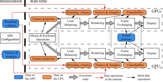
GPUs. There are a total of eight execution components including LOD Selection,
Load Balancing, GPU Out-of-Core, Mesh Reformation, Rasterization, Frame Ex-changing,Synchronization, andDisplay. AABBs and edge-collapsing arrays are pro-duced during the preprocessing stage, and they are sent to GPUs at the initialization of the system. Vertices and triangles are maintained in the CPU main memory, and the LOD selected data portions will be transferred to GPUs at the runtime. The screen portions that are generated at the runtime will be exchanged among GPUs with a direct inter-GPU communication technology. . . 49 4.4 A dual-GPU load balancing example. It finds the screen partitioning line dividing the
LOD selected triangles in the view frustum of the full screen into two sub-frustums. The numbers of triangles in the sub-frustums are balanced, and the triangles in each sub-frustum are rasterized by one GPU. . . 52 4.5 The execution of the GPU out-of-core component, illustrated with two GPUs and five
objects. Obj0andObj1are handled byGP U0, andObj2,Obj3, andObj4 are handled
byGP U1. The bright orange blocks represent the LOD selected data portions out of
the full object data, which are the portions needed by the current frame. The data of the previous frame (dark orange blocks) are already on the GPUs, so they do not need to be transferred. The CPU collects the frame-different data (blue blocks) and then transfers them to the GPU memory. After that, the frame-different data and the data of the previous frame are merged to construct the data of the current frame. 54 4.6 An example illustrating the Frame Exchanging component in a system with three
GPUs. The GPU tree shows the GPU configuration which includes two vertical screen-partitioning lines. . . 57 4.7 The workstation we built with four GPUs and four display monitors. It supports
the customized rendering of complex polygonal models using one, two, three, or four GPUs, where each GPU connects to one display monitor. . . 58 4.8 The performance over different values of N. The FPS is averaged over 1200 frames.
4.9 Frame-by-frame performance comparison over 1,200 frames of the camera path. The comparison was done on the quad-GPU system. The testing scene is composed of 35 Power Plant models. For the implementations with LOD, N is equal to 50 million, and for the implementations with load balancing, stripN um is equal to 2048. All implementations have the GPU out-of-core enabled. (a) is the comparison between our approach (Load Balancing + LOD) and the LOD Only implementation. (b) is the comparison between our approach and the Load Balancing Only implementation. 65
4.10 The efficiency comparison charts among our approach (Load Balancing + LOD), theLOD Only implementation, and the Load Balancing Only implementation with differentN values. The comparison was done on the quad-GPU system. The testing scene is composed of 35 Power Plant models. The data points are the averaged values over the 1,200 frames of the camera path. For the implementations with LOD, the increment ofN is 5 million. For the implementations with load balancing,
stripN um is equal to 2048. (a) shows the FPS. (b) shows the maximum difference of triangle counts between any two GPUs. (c) shows the rendering time which is the sum of execution time of theRasterization,Synchronization, andFrame Exchanging
components. . . 68 4.11 The influence of different stripN um values on the frame rate on the quad-GPU
system for the scene composed of 35 Power Plant models. Each data point associated with the execution time of the load balancing algorithm. The value in the parenthesis is the percentage that the algorithm’s execution time takes out of the total execution time. N is equal to 50 million. . . 69 4.12 The system performance comparison between the use of our load balancing algorithm
and the use of binary search algorithm with 30 Power Plant model. Each data point also associates with the execution time of the algorithm. The value in the parenthesis is the percentage that the algorithm eection takes out of the total execution time (N
= 40M) . . . 70 4.13 The rendering results rendered by our approach with different N values and the
original rendering [35] (without LOD). (a) is the rendering result withN is equal to 3 million, (b) is the rendering result withN is equal to 60 million, (c) is the original rendering result. The images in the red rectangles are the zoom in screenshots of the far away objects taken by a reference camera. . . 72
5.1 The overview of the crowd multi-GPU rendering system. . . 79 5.2 The examples showing different levels of detail for seven source characters. From top
to bottom, the numbers of triangles are: (a) Alien: 5,688, 1,316, 601 and 319; (b) Bug: 6,090, 1,926, 734 and 434; (c) Daemon: 6,652, 1,286, 612 and 444; (d) Nasty: 6,848, 1,588, 720, and 375; (e) Ripper Dog: 4,974, 1,448, 606 and 309; (f) Spider: 5,868, 1,152, 436 and 257; (g) Titan: 6,518, 1,581, 681 and 362. . . 81 5.3 An example showing the process of unfolding a cube mesh and mapping it into a
flatten patch in 2D texture space. (a) is the 3D cube mesh formed by 8 vertices and 6 triangles. (b) is the unfolded texture map formed by 14 pairs of texture coordinates and 6 triangles. Bold lines are the boundary edges (seams) to cut the cube, and the vertices in red are boundary vertices that are mapped into multiple pairs of texture coordinates. In (b), ui stands for a point (si, ti) in 2D texture space, and vi in the parenthesis is the corresponding vertex in the cube. . . 85 5.4 An example illustrating the data structures for storing vertices and triangles of three
instances in VBO and IBO, respectively. Those data are stored on the GPU and all data operations are executed in parallel on the GPU. The VBO and IBO store data for all instances that are selected from the array of original vertices and triangles of the source characters. ThevN um and tN umarrays are the LOD section result. . . 87 5.5 An example of the rendering result produced by our system using differentN values.
(a) shows the captured images with N = 1,6,10 million. The top images are the rendered frame from the main camera. The bottom images are rendered based on the setting of the reference camera, which aims at the instances that are far away from the main camera. (b) shows the entire crowd, including the view frustums of the two cameras. The yellow dots in (b) represent the instances outside the view frustum of the main camera. . . 92 5.6 The change of FPS over different values of N by using our approach. The FPS is
averaged over the total of 1,000 frames. . . 93 5.7 The performance comparison of our approach, pseudo-instancing technique and
point-based technique over different numbers of instances. Two values ofN are chosen for our approach (N = 5 million and N = 10 million). The FPS is averaged over the total of 1,000 frames. . . 94
5.8 The visual quality comparison of our approach, pseudo-instancing technique and point-based technique. The number of rendered instances on the screen is 20000. (a) shows the captured image of our approach rendering result withN = 5 million. (b) shows the captured image of pseudo-instancing technique rendering result. (c) shows the captured image of the point-based technique rendering result. (d), (e) and (f) are the captured images zoomed in on the area of instances which are far away from the camera. . . 95 5.9 Crowd rendering performance over different values of N. The FPS is averaged over
1200 frames. The increment ofN is 5M and stripN um= 2048. . . 98 5.10 The performance comparison between the use of our approach and the
hardware-accelerated psedo-instancing approach using quad-GPU. The chart is for the crowd rendering withstripN um= 2048 andN = 10M. . . 98
3.1 Performance breakdowns for the system with stripN um = 2048. “—” in the table indicates that the component is not applicable or the workstation with given “# of GPUs” does not have sufficient memory to hold selected vertices and triangles. . . . 37 3.2 Performance breakdowns for the system at different screen resolutions. A total of 15
Power Plant models (32.81 million vertices and 75.86 million triangles) are rendered, and the values in the table are averaged over 1200 frames. . . 37
4.1 Performance breakdown of our approach with stripN um is equal to 2048. A total of 35 Power Plant models (210.20 million vertices, 444.65 million triangles and 5.29 million objects). The values are averaged over 1,200 frames. “—” in the table indicates that the component is not applicable or the workstation with given “# of GPUs” does not have sufficient memory to hold the selected vertices and triangles. . 60 4.2 Performance breakdown of our approach at different screen resolutions on the
quad-GPU system. A total of 35 Power Plant models (210.20 million vertices, 444.65 million triangles and 5.29 million objects) are rendered. N is equal to 50 million. The values in the table are averaged over 1,200 frames. . . 61 5.1 The data information of the source characters used in our experiment. Note that the
data information represents the characters that are prior to the process of UV-guided mesh rebuilding (see Section 5.4.2). . . 90
5.2 Performance breakdowns for the system with a pre-created camera path with total 30,000 instances. The FPS value and the component execution times are averaged over 1000 frames. The total number of triangles (before the use of LOD) is 169.07 million. . . 91 5.3 Performance breakdowns for crowd rendering with stripN um = 2048. A total of
20000 animated characters (66.62 million vertices and 112.63 million triangles). The values are averaged over the 1200 frames. “—” in the table indicates that the com-ponent is not applicable in single GPU system. . . 97
Introduction
Real-time rendering is a major component in computer graphics. In many research and industrial areas, such as computer-aided design (CAD), manufacturing, video game development, scientific visualization, and virtual reality, the rendering of complex 3D geometric data sets in real-time is fundamental in interactive applications. Engineers, scientists, or game players need to interact with 3D models from any angle by moving the mouse and pushing a button to zoom in or out for close-up or long-distance views. Due to advances in 3D modeling, data acquisition, and simulation technologies, 3D data sets continue their explosions in both quantity and complexity. It has become common that a 3D model consists of millions, even hundreds of millions of vertex and triangle primitives. In order to achieve efficient storage management, vertices and triangles are usually grouped in objects. An object is a self-contained and fully functional design part. To have a complete description of the design, the model may contain thousands, or hundreds of thousands, of such objects, just like Kenneth Wong stated in his article [162] that, “Before, if you’ve got 1,000 parts, that was big. Now, we’re talking about assemblies with 10,000, 15,000 or hundreds of thousands of parts. That has become the norm.”
Interactive data visualization results in new discoveries. It reveals patterns and significance in data that people may otherwise have missed. A satisfactory interactive experience requires rendering performance to be at an interactive frame rate (e.g. 20 frames per second or above [10]), but achieving high rendering performance for a large data set is challenging because it is time-consuming to convert a huge amount of triangles into pixels on the screen at each time a frame being rendered. In the past two decades, with the rapid improvements on graphics hardware, graphics processing units (GPUs), as a massively parallel architecture and a commodity computing platform, have
been praised for the significant performance increase at a low cost and the capability to perform general-purpose parallel computations. Many visualization applications for large data sets have been redesigned with GPU-friendly parallel implementations, such as examples mentioned in [16,17]. In recent years, the motherboard in a workstation can be configured with multiple PCI Express (PCIe) slots that enable the installations of two or more graphics cards. This configuration can increase the overall system performance by distributing workloads across multiple GPUs. Also, with additional GPU display ports, multiple display monitors can be connected, so that rich information embedded in the large data set can be rendered at higher resolutions, as they should deserve. Hence, designs of a scalable real-time rendering system using multiple GPUs and multiple dis-plays supporting the rendering of complex 3D environments will benefit the manufacturing and visualization area in achieving high performance and high resolution rendering results efficiently.
1.1
Motivation
Nowadays, as human-computer interaction studies improve, people need not only static rendering results but highly interactive experience and high display resolution of the complex 3D data set. For instance, mechanical engineers may want to modify some parts of an automobile design interactively and immediately see the changes; scientists may want to change parameters in a simulation and see the updated data rendering immediately. 3D data sets are usually represented as a set of triangles, where each triangle is composed of three vertices defining their positions in 3D space. Triangles are interconnected with shared vertices and edges. As a result, the set of triangles forms a mesh topology that describes the structure and shape of an object.
Over the last two decades, the evolution of GPU architectures has resulted in billions of processing transistors per chip and allow to launch of millions or even billions of threads (fine-grained paral-lelism) to process a massive amount of elements simultaneously. GPUs are optimized for single-instruction multiple-data (SIMD) operations. The graphics rendering pipeline in modern GPUs has been developed to support parallel execution of the standard rasterization algorithm [3, 134, 154], where all triangles can be shaded and then converted into pixels with fine-grained triangle-level parallelism. This rendering pipeline requires vertices and triangles to be transferred from CPU main memory to GPU memory before they can be rasterized. As the data set grows, GPUs suffer memory size limitations. In comparison to the size of CPU main memory, GPU memory is much smaller. For example, the common CPU memory of a commodity workstation is 64 GB, but the common memory of a GPU is only 8 GB. Thus, a large data set that can be stored in CPU memory
1M
10M 100M 1B
1
10
100
1000
Data Size
Performance (fps)
OpenGL 3D graphics hardware: f(P) = 1/P
Visibility-guided rendering: f(P) = 1/log(P)
Figure 1.1: The performance comparison between traditional rendering and visibility culling meth-ods. [81]
may not fit into GPU memory. In such cases, data has to be transferred in multiple passes, and the GPU has to render the data in each pass with a separate drawing call. Because data transfers and drawing calls have to be executed at each time a frame is being rendered, the system will suffer a lot on performance, or it may even fail the rendering.
To reduce the transferred data size and avoid having multiple passes when transferring data in multiple passes, GPU-based acceleration techniques have been proposed, such as adaptive level-of-detail (LOD) methods [31, 32, 71, 129], visibility culling methods [9, 62, 150] and GPU out-of-core streaming methods [22, 33, 57, 128, 168], to reduce the amount of data to a size that is small enough to fit into GPU memory and able to send in a single pass, while maintaining the visual fidelity of the rendering. In particular, LOD methods reduce the geometry complexity of the objects that are far away from the camera; visibility culling methods reduce the complexity of the rendered scene by rejecting the objects that locate out of the camera view. Both acceleration techniques increase the rendering performance by reducing the total amount of triangles in the rendering pipeline, as shown in Figure 1.1. Therefore, the amount of data in the entire scene can be reduced and retained in the GPU memory.
The number of polygons that contribute to the rendered image is limited by the total number of pixels available on the display. Although the acceleration techniques can improve the GPU’s
(b)
(a)
Figure 1.2: Examples of complex 3D models. (a) is an array of 20 duplicated UNC Power Plant model composed of approximately over 120 million vertices and 254 million triangles organized in over 3 million objects. (b) is a large crowd rendering composed of 30,000 animated characters containing over 100 million triangles.
ability to handle a data set larger than the GPU memory capability, with a single GPU, the display resolution may not provide a sufficient number of pixels to represent the rich information in the complex data set. The highest display resolution is bounded to the maximum number of pixels that the display monitor provides. However, even if each triangle is rasterized to one-pixel size, in theory, only a maximum of 8.3 million triangles can fit on a 4K screen (3840×2160 pixels). The screen has far less than enough pixels to display the large model composed of hundreds of millions of triangles.
There are two types in a typical complex 3D environment — static scene and dynamic scene. For example, a static scene usually composed of a large-scale of massive 3D polygon models, as shown in Figure 1.2 (a), and a dynamic scene usually composed of a large number of animated characters or objects distributed in the scene, as shown in Figure 1.2 (b). Both of the two types have the difficulty of rendering efficiently because of the limited memory capability of a single GPU and limited resolution of a display monitor, in this dissertation, I spent my efforts to research on parallel algorithms and data management methods that can take hardware advantages of a multi-GPU multi-display rendering system for the complex 3D environment. The total size of GPU memory is increased and distributed across multiple GPU cards in this system. Each GPU may drive one or more display monitors so that together they form a large tiled display. The delivered system supports the task of rendering the complex 3D environment composed of hundreds of millions of triangles at highly interactive frame rates.
1.2
Challenges in Multi-GPU
Researchers have studied parallel rendering methods with multiple GPUs recently. The advan-tage of using multiple GPUs is that the size of available GPU memory, display resolution, and computational power can be increased. The workload and task to render a large data set can be to distributed among multiple GPUs, and the rendered image can be projected to a large tiled display, where each tile is one display monitor connected to a single GPU device. However, the state-of-the-art solutions do not achieve the computational power and display resolution increasing proportionally to the number of GPUs installed.
In this section, I describe three research challenges that I believe are important computing issues in multi-GPU based visualization applications as well as for parallel computing in general.
Load Balancing Among GPUs
The first and most important problem that needs to be addressed in a multi-GPU system is how to balance the workload distributed among GPUs. When using multiple GPUs to increase the total graphics memory, the workload among GPUs needs to be balanced at each time that a frame is being rendered. An imbalanced workload may affect the performance or even fail the rendering tasks. For example, it is very common to see that a large number of objects are rendered to a small region on the screen while other regions are empty. The GPU that deals with more workload and more rendering tasks might need more computational power, and therefore this causes other faster GPUs to stay idle. In an extreme case, one GPU may have to process the entire data set that exceeds the memory capacity, which will fail the whole rendering process. For an interactive rendering application, interactions from the users may create an unpredictable imbalanced workload if they rapidly move the camera or zoom in and out repeatedly. The parallel rendering system can distribute the rendering workload equally in some simple static image rendering tasks. However, in most of the interaction rendering tasks, the system has to redistribute workload among GPUs in every frame dynamically.
Inter-GPU Communication
By distributing data among GPUs, the entire scene is no longer abided by a single GPU. A frame rendered by a GPU may need to be displayed on the display monitor that is connected to a different GPU. Thus, all GPUs in the system need to communicate with each other and transfer data from one GPU to another at run-time. However, transferring the entire or partial geometry data is very time-consuming. The current existing GPU does not have enough bandwidth to transfer such large data. Parallelizable tasks usually incur a non-parallelizable overhead [7]. In a parallel rendering system, people have to struggle with the additional performance overheads caused by inter-GPU communication and synchronization. Such overheads become more significant as the number of GPUs and the display resolution increase.
Interactive Rendering with Acceleration Integration
In a complex 3D scene, it is not necessary to render the fine details of objects when they are far away from the camera’s viewpoint. Reduce the complexity of the occluded and long-distance objects can save computational power. Many solutions have been implemented successfully on a single
GPU. However, migrating the traditional acceleration techniques from a single GPU to multiple GPUs is a challenge. The complexity of 3D models is difficult to determine due to the different transformation matrices and different data locations among GPUs. Integrating state-of-the-art parallel LOD, visibility culling and GPU out-of-core techniques into a multi-GPU multi-display system has not been successfully addressed.
1.3
Contribution
In this dissertation, my research work will contribute to the fields of high-performance graphics, massive model rendering, and multi-GPU based parallel computing. The outcome of this work is to advance the state-of-the-art by optimizing the use of distributed GPU memory without the requirement of data replication, exploring the potential of novel technology to improve the rendering performance and increase the resolution. In particular, I conduct multi-GPU multi-display research on commodity workstations, in which each GPU connects to one or more display monitors, and together to form a large tiled display at low costs. The system enables the per-GPU per-display setting and can process and render large 3D data sets in a fine-grained parallel scheme, without the requirement of using complex hierarchical data representations. The system has good scalability to allow an arbitrary number of GPUs to handle the data set efficiently with a growing number of vertices and triangles.
The following contributions are presented as part of this dissertation:
1. Improving the rendering performance by balancing the workload among GPUs before the rendering stage of each frame. In order to fully utilize the computational power and available memory of each GPU, I present a novel load balancing algorithm to dynamically partition the entire data set based on certain view-dependent criteria in order to fully utilize the computational power and available memory of each GPU in the system. This algorithm is able to help to improve the overall performance of the rendering system by ensuring the amount of data (vertices and triangles) handled by each GPU is balanced. In particular, the algorithm finds a partitioning line on the screen to balance the amounts of data appearing on the partitioned portions of the screen. Each GPU only needs to load and render the data appearing on one portion of the screen. The execution of this algorithm is efficient and does not counteract the performance increased from the load balancing.
transferred between GPUs. The key idea to minimize the inter-GPU communication cost is to reduce the amount of transferred data. Although the PCIe bus for transferring data from one GPU to another GPU is slower than other hardware solutions in terms of the data transfer throughput, it is still the state-of-the-art technology that allows each GPU to retain unique (non-replicated) data elements. However, a brute-force data transfer will lead to a large overhead on the PCIe bus. I develop an algorithm that allows a GPU to transfer only a small portion of the rendered frame, rather than the full-frame or geometry data, so that the overhead of inter-GPU communication can be reduced. Comparing to the size of the original data, a portion of the rendered frame is much smaller, composed of a small amount of pixels. 3. Integrating parallel level of detail, visibility culling and out-of-core acceleration techniques in the multi-GPU multi-display rendering system. Loading and rendering only visible objects at a simplified but visually-satisfied level of complexity is an important ac-celeration technique for real-time rendering. I employ a suitable GPU-friendly data structure to enable parallel LOD, visibility culling, and out-of-core techniques for multi-GPU rendering system, without using complicated hierarchical data representations. Invisible or unneces-sary objects and geometry primitives will be eliminated from the rendering pipeline. Visible objects will be appropriately simplified according to certain view parameters and streamed from CPU main memory to GPU memory with a frame-coherent strategy while maintaining high visual fidelity of the rendering.
4. Supporting rendering of both static and dynamic 3D environment in high per-formance and high resolution. Rendering multiple types of 3D data is necessary for a rendering system. The multi-GPU multi-display rendering system I present has the ability to render both static CAD models and the dynamic animated crowd. I also thoroughly evaluated the performance and efficiency of the system in detail.
1.4
Organization
The remaining part of this dissertation is organized as follows. Chapter 2 gives an introduction to the topic of parallel rendering. State of the art is reviewed. Chapter 3 presents a novel screen partitioning load balancing algorithm that dynamically distributes the workload among GPUs and an efficiency inter-GPU communication method that only transfers a small portion of the rendered frame to reduce the overhead. Chapter 4 presents a multi-GPU multi-display rendering system to render an extremely complex 3D environment. The system is featured with GPU-friendly
performance and scalability techniques, including inter-device load balancing, coherence-based GPU out-of-core, and parallel level-of-detail. Chapter 5 presents a large dynamic crowd rendering system with integration of the feature of level-of-detail, load balancing, and frame exchanging using multiple GPUs. The system shows that the proposed multi-GPU multi-display system has the ability to render both static and dynamic 3D environments. Chapter 6 concludes the work presented in this dissertation and propose future work.
Multi-GPU Rendering Tools and
Methods
As the complexity of 3D models keeps increasing, the complex 3D environment’s data size and the computational power for rendering such scenes are exploding. The benefit of scalable memory size and resolution provided by parallel rendering with multiple GPUs approaches have attracted many researchers. A variety of approaches and systems built on the foundation of multi-GPU have been developed. In this chapter, I will review the state-of-the-art solutions for parallel rendering with multiple GPUs.
2.1
Solutions with Distributed Clusters or Supercomputers
Distributed clusters or supercomputers are used to solve big data problems. They are usually used for diverse heavy scientific and general-purpose computing applications, rather than focusing on visualization applications. Recently, Ahrens et al. [2] proposed to add separate visualization nodes in a distributed computing system to display result images. The visualization nodes have to communicate with the main nodes to fetch the result images. Grosset et al. [59] introduced a GPU-based image compositing algorithm to reduce the communication time between nodes in the supercomputers for scientific visualization. Bethel et al. [15] discussed the challenges and efforts to maintain the visualization infrastructure on supercomputers. In general, establishing and Maintaining supercomputers usually require a large investment in human resources and funds. Wagstaff stated in his article inTIME.com [156] that “Aside from the $6 to $7 million in annual
energy costs, you can expect to pay anywhere from $100 million to $250 million for design and assembly, not to mention the maintenance costs.”
Distributed clusters or supercomputers are normally more complicated to use than commodity desktop workstations. Distributed clusters or supercomputers are not suitable for visualization and interaction tasks due to the nature of batch mode executions. A significant amount of additional effort would be needed to modify the architecture of the supercomputer if intending to make it capable of visualization and interaction. Alternatively, GPUs installed in normal, off-the-shelf desktop workstations have the potential to provide competitive computational power at vastly lower costs. The recent GPU computing technologies have been praised not only for the significant performance increase but also for the capability to perform both graphical and general-purpose computations.
2.2
Hardware Solutions
Hardware solutions utilize specialized devices or acceleration hardware chips on GPUs to improve the GPUs’ efficiency when executing the standard graphics rendering pipeline. Recently, bridging circuit boards have been developed to directly connect GPUs in order to improve the data com-munication efficiency between GPUs. Instead of transferring the GPU data back to the CPU main memory and then transferring it to another GPU through PCIe buses, the data can go through a faster and direct path on the bridge board plugged between the two GPUs.
NVIDIA SLI [121] and AMD CrossFire [6] are popular bridging circuit boards commercially avail-able for parallel rendering with multiple GPUs in a single workstation. Their design idea is similar. They configure GPUs as one hardware entity using the circuit board. As a result, multiple GPUs installed on the motherboard are able to share the workload at the run-time of the system. When the SLI or CrossFire is enabled, one GPU has to be treated as the master device; and other GPUs become workers. After receiving rendering results from the workers transferred through the bridge, the master GPU combines the results and displays the composited image on the screen. This master-worker configuration mainly supports two types of rendering modes in both brands: (1) Split Frame Rendering (SFR) and (2) Alternate Frame Rendering(AFR) [120]. In AFR, as shown in 2.1 (a), each GPU renders the entire screen in a successive order of frames. For example, in a dual-GPU configuration, one GPU renders the odd number of frames, and the other GPU renders the even number of frames. After a GPU finishes the rendering task, the rendered result is sent to the master GPU, and then the master GPU displays it on the screen. In AFR, the master
Frame
n Frame n+1 Frame n+2 Frame n+3 Frame n+4 Frame n+5
(a)
(b)
Frame
n Frame n+1 Frame n+2 Frame n+3 Frame n+4 Frame n+5
Figure 2.1: The example of two rendering modes in SLI. (a) is the Alternate Frame Rendering (AFR) mode. (b) is the Split Frame Rendering (SFR) mode.
GPU does not need to perform the image composition task. In SFR, as shown in 2.1 (b), the master analyzes the rendered image and splits the screen into multiple regions where each region can be handled by a worker GPU. For example, in a dual-GPU system, the render target may be divided vertically or horizontally. Each GPU responds to a half region of the whole scene. After all GPUs (including all workers and the master) finish the rendering of their regions, worker GPUs’ rendered results are sent to the master GPU. Then, the master GPU combines the rendered results. However, these techniques with SLI or CrossFire can not configure a workstation with a per-GPU per-display setting. Only the master GPU is capable of driving display monitors. Thus, the full display resolution is limited by the maximum resolution of the display monitor connected to the master GPU. Furthermore, these techniques do not expand the total size of the GPU memory. They require the same vertices and triangles to be replicated to each GPU. This means that the available memory for storing the original data is not increased.
We can see that, with SLI or CrossFire, the computational cost can be reduced by distributing the workload among GPUs, but the available memory and display resolution are not increased due to the requirement of data replication and the use of a master-worker configuration. Such limitations on memory and display resolutions make the SLI and CrossFire not suitable for the large model rendering applications, which want to use multiple GPUs and multiple displays.
NVLink [48, 119] is a successor of NVIDIA SLI. It is a high-bandwidth communication interface for high-speed GPU-GPU data transferring. NVLink eliminates the master-worker configuration in SLI and enables direct peer-to-peer communication among up to four GPUs in a single workstation. When using an NVLink circuit board, each GPU is allowed to drive a display monitor. The
bandwidth path in NVLink is much more efficient than the PCIe bus between CPU to GPU and also GPU to GPU interconnection [94]. For example, a Tesla V100 features 6 NVLink slots for connecting with three other GPUs at a total GPU-GPU bandwidth of up to 300 GB/s. However, the NVLink technique is enabled only on specific and high-cost GPU devices, including Quadro, Tesla, and Geforce RTX 2080 cards. Similar to SLI, data replication is required by default on NVLink. NVLink does not provide a programmable interface for software developers to easily optimize its usage for data management on GPU memory. This limitation restricts the flexibility in developing customized multi-GPU solutions.
2.3
Middleware Solutions
Middleware is a software layer that gives the operating system access to the applications [55]. In a visualization application, the middleware usually provides an intermediate layer that enables the communication and management of data between GPUs and the visualization applications. Unlike hardware solutions, middleware solutions can control the GPU configuration and distribute workloads without being involved in the hardware’s rendering pipeline.
Eilemann [37] wrote a white paper that summarizes middleware solutions for parallel rendering, including OpenGL Multipipe SDK [18], Chromium [73], Equalizer [40, 41], Omegalib [45], and CAVELib [122]. OpenGL Multipipe SDK (MPK) is a scalable rendering toolkit that implements an effective parallel rendering API to manage the graphics applications in the shared-memory rendering system. It provides a high-level abstraction layer to graphics applications so that they can achieve low-level optimizations. While MPK has the advantage of flexible programming, it only available for a single application on a single node workstation.
Chromium is a cluster-based rendering system, which is based on WireGL [72]. It packages the graphics API commands and provides stream filters to arrange the graphics accelerators [63]. The rendering calls are forwarded to appropriate target GPUs according to different configurations of cluster nodes. The Chromium offers the flexibility of customized implementations but shows scalability bottlenecks because of the serialized streaming calls through multiple nodes. The follow-up system ClusterGL [117] tries to reduce network latency by compressing data but still does not hit the principle structural bottlenecks.
Equalizer [40] is a state-of-the-art parallel rendering framework designed for scalable and flexible multi-GPU configuration for distributed cluster-based parallel rendering system as well as the single
begin frame end frame exit? exit stop init windows exit? stop no exit? stop swap swap
cull / draw cull / draw
exit
windows windowsexit
event handling update data init windows no no
yes yes yes
(b) Application OpenGL OpenGL GPU GPU render render (a)
Figure 2.2: Illustration of Equalizer. (a) is an example of Equalizer application. (b) is an example of an execution flow for Equalizer applications.
shared-memory workstation. It distributes the rendering tasks in parallel on multiple rendering channels, as shown in Figure 2.2 (a). Equalizer offers a transparent layer for controlling rendering resource allocation through a compound tree structure for the GPUs configuration. A client-server model is employed in the framework. A server launches and controls the distributed rendering clients based on a user-provided configuration file at the initialization stage. The clients are responsible for the rendering task and have access to GPUs ( see in Figure 2.2 (b)). Recently, Equalizer 2.0 [41] has been released, and it comes with new performance and scalability features for multi-GPU rendering, such as tiles and chunks rendering and virtual reality support. In particular, Equalizer 2.0 optimizes the inter-GPU communication layer for the data composition. As a generic rendering platform, Equalizer provides various multi-GPU rendering methods, including first 2D rendering, sort-last dynamic balancing rendering, stereo rendering, and multilevel decompositions. However, the biggest limitation of the Equalizer is that it does not have an efficient way to represent and distribute data on GPUs. For example, vertices and triangles have to be represented and managed in a hierarchical data structure, such as bounding volume hierarchy (BVH) [91, 137] and k-d tree [14]. Storing a scene in a hierarchy may require much more memory and much more processing time than
vertices and triangles. For example, in my experiment, it takes more than 20 minutes to build the k-d tree for a scene composed of 15 duplicated Power Plant models and occupies a double memory size of the original vertices and triangles data. Also, the traversal of a hierarchy structure usually leads to large memory footprints for each thread. Moreover, Equalizer targets on the applications of static model rendering, so it lacks the capability to render dynamic or animated scenes.
Omegalib is a framework that provides an abstraction layer for the immersive 2D-3D applications development. It also offers event handling for multiple heterogeneous devices. CAVELib is a soft-ware API to develop virtual reality applications in Cave Automatic Virtual Environments (CAVEs). The original CAVE [28] was introduced with a cube projector-based display driven by a distributed system. It requires a large physical space to set up. The display resolution of a CAVE is limited by the projectors’ resolution. CAVE2 [46] improves the display resolution by using a cylindrical setup of cubic LCD screens instead of projectors. It utilizes the Omegalib as the core graphics imple-mentation and Equalizer as the display controller to achieve the hybrid reality environment. Since CAVEs only targets on the multi-display development and uses other middleware as the graphics core, it does not avoid the normal requirement of data to be replicated to each computing node of the distributed system and involves an intensive computation on the CPU. Also, there is not a scheme to balance computational tasks among the computing nodes.
2.4
Software Solutions
While the hardware and middleware solutions discussed in Chapter 1 are well developed and are able to achieve the real-time rendering demand, these solutions have the common issues of the hardware limitations and difficulty of programming. Researchers have made many efforts on designing parallel rendering systems using multiple GPUs on software solutions.
One pioneer work in parallel rendering was proposed by Whitman [158]. In that work, a parallel algorithm took the advantages of locally cached memory and increased execution efficiency. The fundamental concept of parallel rendering was proposed by Crockett in [27]. The work examined different types of parallelism available in computer graphics applications and discussed the com-mon issues in designing parallel renderers, such as coherence, load balancing, decomposition, and communication.
Graphics pipeline for rendering consists of a geometry processing stage where input geometry primitives are projected to the image plane and a rasterization stage where the projected primitives
are converted into pixels. In the geometry processing stage, each graphics processor is assigned by a set of primitives in parallel. In the rasterization stage, portions of pixels are assigned to processors for calculation. Since the modeling and viewing transformations are arbitrary, an object can fall anywhere on the screen. Thus, the rendering process can be considered as a sorting problem: how are those geometry primitives transferred into pixels? The sorting always happens in three locations of the rendering pipeline: during the geometry processing stage, in the middle of the two stages and during the rasterization stage. Parallel rendering approaches can be classified into three categories [111] based on the ”sorting” location in the graphics pipeline : sort-first, sort-middle, and sort-last, as shown in Figure 2.3.
R G
Redistribute “raw” primitives Graphics database (arbitarily partitioned)
Display
Redistribute screen-space primitives
Redistribute pixle samples or triangles (Pre-transform) Geometry Rasterization (a) Graphics database
(arbitarily partitioned) (arbitarily partitioned)Graphics database
Display Display (b) (c) R R R R R R R G G G G G G G G G G G R R R R
Figure 2.3: The three sorting categories in parallel rendering described in [111]. (a) is the sort-first approach, (b) is the sort-middle approach, (c) is the sort-last approach.
A sort-first approach partitions the screen into disjoint regions and redistributes primitives to those regions before the scree-spaced parameters are known. A sort-middle approach happens in the middle of the geometry processing and rasterization stage. It redistributes parallel processed geometry to different rasterization units. A sort-last approach happens during the rasterization stage. It distributes the rendered-frame, which are the pixels and then compositing them together to form the rendering result.
2.4.1 Sort First Rendering
A sort-first approach is also called tile-sort algorithm. It happens during the geometry processing stage. Each graphics processor operates an entire graphics pipeline and is responsible for rendering a 2D tile of the final view. The common issue in sort-first approach is the load balancing among each processor. The objects may locate in several small regions and the workload exceed the
(a)
(b)
Figure 2.4: The example of software solution implemented by Equalizer [38]. (a) is an example of sort-first approach implemented using 2D Compound in Equalizer. (b) is an example of sort-last approach implemented using DB Compound in Equalizer.
computational power of the corresponding graphics processors. An example of a sort-first approach implemented in Equalizer using 2D Compound is shown in Figure 2.4 (a).
The sort-first algorithm includes the following steps.
1. Objects are assigned to processors arbitrarily.
2. Processor computes the screen-space bounding box of the objects assigned to it and determines their respective tiles in screen spaces.
3. Redistribute objects to the appropriate processors.
4. Perform the remaining geometry-processing and rasterization calculations for the objects.
Samanta et al. [139] introduced a sort-first parallel rendering system running on a PC cluster. Each processor of the system rendered a balanced workload corresponding to a virtual tile on a projector. Abraham et al. [1] proposed a sort-first method along with a time-guided load balancing strategy. At each frame, the display node partitions the screen into several rectangular tiles. The rendering time of each node is recorded at each frame. The screen partitioning position of the current frame is adjusted according to the rendering time spent on the previous frame. The data set is replicated across all renderer nodes. Allard and Raffin [5] utilized hardware shaders to perform sort-first parallel rendering tasks on networked PCs but without considering load balancing issues. Moloney et al. [112] described a scalable sort-first algorithm for dynamic load balancing. The data set
was evenly divided into uniform bricks and distributed between nodes based on the pre-calculated rendering cost on each pixel. Liu et al. [98] proposed a decoupled parallel rendering approach, which separated the rendering stage and compositing stage by adopting a data-partitioning strategy that assigns an arbitrary data portion to each GPU rendering the full-frame. Gao et al. [51] presented a multi-frame prediction algorithm aimed to solve the unstable and sudden changed situation that leads to the unbalanced workload issue. They gathered feedback of multiple frames together to predict the optimized workload distribution strategy among GPUs. However, the prediction in their approach needed a collection of sequence frames and could not handle the other issue in load balancing which is the data streaming issue caused by the sudden camera changing.
The main features of sort-first approach are redistributing the objects at the beginning and pro-cessors can only render a portion of the screen with the entire rendering pipeline. However, the sort-first approach could result in an imbalance loading issue. The objects may clump into regions and workload may fall onto a few processors. This limits the scalability due to the parallel overhead caused by objects rendered on multiple tiles [111, 114].
2.4.2 Sort Middle Rendering
Sort-middle approach happens between the geometry processing stage and the rasterization stage. In a sort-middle approach, the two stages are usually processed on different processors. The prim-itives are arbitrarily distributed to geometry processors and then sent to the rasterizaion stage after transformation calculations. At each frame, the geometry processor classifies the transformed primitives based on their located regions and distributes them to the appropriate rasterizers. Al-though the sort-middle idea is natural and simple, it requires a large computation and high speed of communications, which is not easy to solve in a multi-GPU system. Williams and Hiromoto [160] proposed a sort-middle approach to the Chromium cluster rendering system. The graphics proces-sors only have the rasterization stage in their implementation. The geometry processing stage was moved to the CPU. The approach is suitable for cluster systems but not for the shared-memory workstation because the movement of the large computations to CPU would lead to an overhead and become the bottleneck of the rendering system. Laine and Karras [88] designed a software rendering pipeline on GPU. It optimized each rendering stage of the pipeline by using separate ker-nel operations. Sort-middle mechanisms are always implemented in a customized graphics pipeline recently [83], because of the flexible programming ability and the ease of the procedure control. Kenzel et al. [82] designed a customized software graphics pipeline on GPU. They used a global sort-middle tiled approach by performing dynamic load balancing between the geometry processing
stage and the rasterization stage.
However, modern GPUs have an internally optimized vertex and fragment processing in parallel which results in the sort-middle approach is not suitable for parallelism among multiple GPUs. In particular, driving multiple GPUs distributed across a network of a cluster does not lead to an efficient sort-middle solution as it would require interception and redistribution of the transformed and projected geometry after primitive assembly [138]. When the tessellatoin ratio is high, the communication requirements remain high. And also, there is still a load imbalance issue between rasterization processors if objects are distributed unevenly over the screen space. Thus, parallel ren-dering for multiple GPUs always exploits sort-first or sort-last methods rather the sort-middle [159].
2.4.3 Sort Last Rendering
The sort-last approach happens during the rasterization stage. It decomposes the rendered primi-tives arbitrarily across all graphics processors. Each processor transforms the primiprimi-tives into pixel values and then transfer or exchange these values to other processors to composite them into the final rendering image. However, the compositing step is computationally expensive because of the large number of pixels. For high quality and high-resolution rendering system, such computations would result in a high data transferring overhead. An example of a sort-last approach implemented in Equalizer using DB Compound is shown in Figure 2.4 (b).
Moreland et al. [113] presented a sort-last method for the parallel rendering of large data sets on a tiled display. Their method evenly distributed polygons among all processors in a PC cluster and composed the rendered images for each tile. Wang et al. [157] divided the screen into tiles and removed the compositing stage from the pipeline by using a “compositeless” algorithm. In their approach, the screen is divided into tiles, and each GPU is assigned with the data in the corresponding tile. Erol et al. [44] presented the cross-segment method for load balancing. Their method evaluated the computational time of each GPU spent on the rendering of previous frames and assigned more rendering tasks to the GPUs that had less computational time so that all GPUs could be balanced in terms of computational time. Larsen et al. [90] presented a strategy for multi-image compositing in sort-last rendering. Their method targeted on speeding up the performance in situ visualization. Eilemann et al. [39] analyzed the asynchronous parallel rendering system on hybrid Multi-GPU clusters and evaluated the optimizations for improving the scalability of the system. Steiner et al. [147] distributed rendering tasks to client nodes with work packages for a dynamic load balancing objective. The nodes pull the work packages from a centralized queue at their own need. Their method is adapted to either sort-first and sort-last rendering. The
composition step in sort-last approach is expensive due to the large amount of pixel data processed. For a high-quality, high-resolution image rendering, this could result in a huge interconnect network overhead [113].
Screen Partitioning Load Balancing
Algorithm
While Chapter 2 briefly reviewed the state-of-art approaches in multi-GPU rendering, the major challenge of dynamically balancing distributed workload among GPUs has not been addressed yet. In this chapter, I will present the detail of my novel parallel load balancing algorithm to dynamically partition the entire data set.
3.1
Dynamic Load Balancing
Evenly partitioning the screen and mapping the partitioned regions to display monitors cannot balance the triangle amounts in those screen regions. While the camera changes its position and orientation during the run-time, the number of triangles in one screen region could be significantly larger than those in other screen regions; and consequently, this leads to a severe load imbalanced issue. The load balancing algorithm aims to find an appropriate partitioning position so that for objects projected on the partitioned regions of the screen, the number of triangles in each partitioned screen region can be balanced.
The load balancing algorithm takes the view frustum and the triangle counts in objects as input. Each GPU executes an instance of the algorithm. The view frustum corresponds to the full screen projected on the entire tiled display, so all GPUs have the same input view frustum. The triangle counts in objects are presented in an array structure, denoted as T, where Ti is the number of
triangles of the ith object. The load balancing algorithm crops the view frustum into a sub-frustum for the GPU and correspondingly modifies the values of the T array for the GPU. As a result, only the objects inside the sub-frustum of the GPU will remain their triangle counts in the
T array. In other words, if theith object is outside the sub-frustum of the GPU, the algorithm will changeTi to zero.
The sub-frustums of all GPUs may be in different sizes, but their triangle counts are balanced. The balancing process is performed in screen space on the near plane of the view frustum. We first introduce the idea of screen and frustum strips in Section 3.1.1. We then describe the load balancing algorithm and its parallelization in Section 3.1.2.
3.1.1 Screen and Frustum Strips
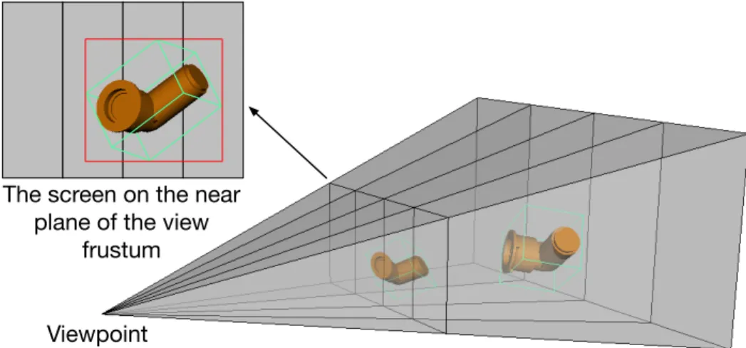
The first step in this method is to partition a screen. The essential operation of screen partitioning is to specify a partitioning line, which cuts through the screen either horizontally or vertically. The choices to specify a partitioning line are limited to the screen resolution. For example, given a dual-GPU workstation with the 1×2 configuration for their monitors, the full-screen will be partitioned vertically. If the screen resolution of each GPU is 1024×768 pixels, the full-screen resolution is 2048×768 pixels. Thus, there are a total of 2048 possible partitioning lines, with each at one pixel on the width dimension. On the near plane of the view frustum, those partitioning lines produce
screen strips, which are small screen regions of the same size. Then, we use the screen strips to subdivide the view frustum intofrustum strips, which are small truncated pyramid volumes created from the screen strips and the viewpoint position of the camera. Like the example illustrated in Figure 3.1, the screen is evenly partitioned into four screen strips, and correspondingly four frustum strips are created.
We define a parameter calledstripN um, ranging in (2, Q), to control the number of frustum strips on each screen axis, where Q is the total number of pixels along this axis. A higher value of
stripN um gives more and narrower strips, and the load balancing algorithm can, therefore, use them to produce a finer balancing result.
3.1.2 Load Balancing Algorithm and Parallelization
The goal of the load balancing algorithm is to find an appropriate partitioning line so that for the objects projected on the partitioned regions of the screen, their triangle counts are balanced. In
Viewpoint
The screen on the near plane of the view
frustum
Figure 3.1: Four frustum strips generated by evenly partitioning the screen into four regions. The red rectangle on the near plane is the bounding rectangle of the projected object’s bounding volume.
a multi-GPU rendering system, GPUs are hierarchically grouped into a binary search tree. This requires a repetitive execution of a partitioning operation in order to progressively update the modified triangle counts T (denoted asT0) and sub-frustums in descendent tree nodes, as shown in Algorithm 1. The number of partitioning operations that a GPU should perform is equal to the depth of this GPU (the corresponding leaf node) in the tree. In order to ensure all GPUs receive the balanced workload, the intermediate partitioning operation for a non-leaf node is weighted based on the number of GPUs that its two child nodes contain. Here, we introduce a term for such weighting called balRatio, so we have balRatio = P arInf oi.ncl
P arInf oi.ncr, where i is theith partitioning
operation that associates to the non-leaf node. After each iteration of screen partitioning, the value ofbalRationeeds to be recalculated (see line 4 in Algorithm 1). The partitioning operation takes the computed balRatio, the sub-frustum, bounding volumes of objects, and triangle counts as input, and then finds the screen partitioning position (p-pos of this non-leaf node (see line 5 in Algorithm 1). As a result after all iterations of screen partitioning, we obtain an array of p-pos
values, where eachp-pos value corresponds to the result of a screen partitioning operation.
Here, we want to explain the single step algorithm executed at each iteration of screen partitioning. Figure 3.2 illustrates the execution of the algorithm using an example composed of 16 frustum strips and 10 objects. Note that the triangle count of each object is already known and retrieved from Ti. The GPU allocates two arrays in the memory whose sizes are equal to the number of frustum strips. The first one is called Start array, denoted as S; and the second one is End array, denoted as E. Si is the sum of triangle counts of the objects intersecting with the ith strip, and thisith strip must be the first strip the objects intersect with. Ei is also the sum of triangle counts
20 T3 12 T1+T9 23 T7 15 T4 5 T0 30 T5 30 T2+T6 8 T8 22 T3+T9 10 T1 15 T4 28 T0+T7 30 T5 18 T6 12 T2 8 T8 20 20 20 32 55 70 70 75 105 105 135 143 143 143 143 143 143 143 143 143 121 121 111 96 68 68 38 38 20 8 8 8 0.86 0.86 0.86 0.74 0.55 0.37 0.27 0.10 0.54 1.76 2.55 16.88 16.88 16.88 0 1 2 3 4 5 6 7 8 9 10 11 12 13 14 15 0 1 2 3 4 5 6 7 8 9 10 11 12 13 14 15 0 1 2 3 4 5 6 7 8 9 10 11 12 13 14 15 0 1 2 3 4 5 6 7 8 9 10 11 12 13 14 15 Obj9 T9=2 Obj1 T1=10 Obj4 T4=15 Obj7 T7=23 Obj5 T5=30 Obj0 T0=5 Obj6 T6=18 Obj2 T2=12 Obj8 T8=8 Obj3 T3=20 6.15 S E Prefix-sum operation Diff S E
+∞
Figure 3.2: An example of the load balancing algorithm for a non-leaf node in the GPU tree. A total of 10 objects are projected on the screen. The stripN um is set to 16. Assume that the number of GPUs in two child nodes of this non-leaf node is same , so that the value ofbalRatiois equal to 1.0.
Input: V iewF rustum,BoundingV olumes,T,stripN um,depth;
Output: T0, an array ofp-pos) 1: T0←T;
2: sub-frustum ←V iewF rustum; 3: fortheith level of thedepthdo
4: balRatio← P arInf oi.ncl
P arInf oi.ncr;
5: {T0, p-posi, sub-frustum} ← SingleStepPartitioning(sub-frustum, BoundingV olumes,
T0,balRatio,stripNum); 6: end for
of the objects intersecting with the ith strip, but this ith strip must be the last strip the objects intersect with. In Figure 3.2, we haveS3 =T1+T9 because onlyObj1 andObj9 use the third strip
as the first intersected strip. If an object crosses the left boundary of the screen, we assume the first strip is the left-most strip (e.g., Obj3 in Figure 3.2). Similarly, if an object crosses the right
boundary of the screen, we assume the last strip is the right-most strip (e.g., Obj8 in Figure 3.2).
Algorithm 2 shows the single step of screen partitioning with object-level parallelization. The algorithm returns the modified triangle countsT0, the screen partitioning position (p-pos), and the sub-frustum that will be used by the next level of partitioning. The value ofp-pos is a normalized value ranging in [0,1]; so if the value of p-pos is equal to 0.5, it indicates the view frustum is divided at the middle. The algorithm first needs to find out the strips that an object interests. As shown in Figure 3.1, the intersection test is performed in screen space using the bounding rectangle of the object’s projected bounding volume. According to the theory of perspective projection in computer graphics, if the bounding rectangle of an object intersects with a screen strip, the bounding volu


![Figure 2.3: The three sorting categories in parallel rendering described in [111]. (a) is the sort-first approach, (b) is the sort-middle approach, (c) is the sort-last approach.](https://thumb-us.123doks.com/thumbv2/123dok_us/1080687.2643774/35.918.107.809.415.647/figure-categories-parallel-rendering-described-approach-approach-approach.webp)