Epidemiological Prediction using Deep Learning

(1)

저작자표시-비영리-변경금지 2.0 대한민국 이용자는 아래의 조건을 따르는 경우에 한하여 자유롭게 l 이 저작물을 복제, 배포, 전송, 전시, 공연 및 방송할 수 있습니다. 다음과 같은 조건을 따라야 합니다: l 귀하는, 이 저작물의 재이용이나 배포의 경우, 이 저작물에 적용된 이용허락조건 을 명확하게 나타내어야 합니다. l 저작권자로부터 별도의 허가를 받으면 이러한 조건들은 적용되지 않습니다. 저작권법에 따른 이용자의 권리는 위의 내용에 의하여 영향을 받지 않습니다. 이것은 이용허락규약(Legal Code)을 이해하기 쉽게 요약한 것입니다. Disclaimer 저작자표시. 귀하는 원저작자를 표시하여야 합니다. 비영리. 귀하는 이 저작물을 영리 목적으로 이용할 수 없습니다. 변경금지. 귀하는 이 저작물을 개작, 변형 또는 가공할 수 없습니다.

(2)

Master’s Thesis

Epidemiological Prediction using Deep Learning

Jaewoong Heo

Department of Mathematical Science

Graduate School of UNIST

(3)

Epidemiological Prediction using Deep Learning

Jaewoong Heo

Department of Mathematical Science

(4)

(5)

(6)

Abstract

Accurate and real-time epidemic disease prediction plays a significant role in the health system and is of great importance for policy making, vaccine distribution and disease control. From the SIR model by Mckendrick and Kermack in the early 1900s, researchers have developed a various mathematical model to forecast the spread of disease. With all attempt, however, the epidemic prediction has always been an ongoing scientific issue due to the limitation that the current model lacks flexibility or shows poor performance. Owing to the temporal and spatial aspect of epidemiological data, the problem fits into the category of time-series forecasting. To capture both aspects of the data, this paper proposes a combination of recent Deep Leaning models and applies the model to ILI (influenza like illness) data in the United States. Specifically, the graph convolutional network (GCN) model is used to capture the geographical feature of the U.S. regions and the gated recurrent unit (GRU) model is used to capture the temporal dynamics of ILI. The result was compared with the Deep Learning model proposed by other researchers, demonstrating the proposed model outperforms the previous methods.

(7)

(8)

List of Figures

1 Feed forward network . . . 7

2 RNN . . . 11

3 LSTM . . . 12

4 GRU . . . 13

5 CNN . . . 15

6 Graph, adjacency and feature matrix . . . 16

7 ILI Activity map [1] . . . 19

8 Data used for the evaluation [2] . . . 20

9 RMSE change for train and test . . . 25

10 CORR change . . . 25

(10)

I

Introduction

Epidemiology is the study of the distribution and determinants of the health-related states or events, and the application of this study can be used to the control of disease or other health problem [3]. The concerning infectious disease is caused by pathogens such as bacteria, virus, or fungus and the infected host act as a secondary medium for the transmission of the disease. This medium includes water, air, or living organisms such as mosquitos which is the major cause of various diseases including dengue fever and Zika. Due to its high spreading ability, the infectious disease is a major concern in public health. Recently, there were several major outbreaks such as SARS, swine flu and MERS and the annual global cost of such pandemics is estimated to be over $570 billion [4].

Mankind effort to predict such disease has a long history, starting from 400 B.C. Athens philosopher Hippocrates’s attempt to explain the role of environment and host in spreading of the disease to the 1800s anesthesiologist John Snow’s systemic work for investigation of the prevalence of cholera. The milestone in explaining the spread of disease using mathematics was set by Mckendrick and Kermack in 1927. For most of the disease, the host gets the immune system after it cured. Based on the fact, the two scientists translated the dynamics of disease into three representations: susceptible(S), Infected(I), and Removed(R). Assuming the number of people isN and there is no change from birth or death, the total number of the sum ofS(t),

I(t) and R(t) is kept the same for all time. With appropriate choice of the transmission rate (S → I) and recovery rate(I → R), the SIR model can be solved using ordinary differential equation [5]. dS dt =−βSI (1) dI dt =βSI −αI (2) dR dt =αI (3) S(t) +I(t) +R(t) =N (4)

Above equations are the basic SIR compartment model which was introduced by Mckendrick and Kermack where the β represents the transmission rate and α the recovery rate. Here, the variables and parameters are positive. The SIR model can be simplified or altered according the types of disease. For example, chronic disease such as herpes cannot be cured hence it fits SI model which stated below [5].

(11)

dS dt = −βSI N (5) dI dt = βSI N =βI(1− I N) (6)

For the case of sexually transmitted disease such as chlamydia, the pathogen does not confer immunity. Therefore, SIS model fit into this category [6] since the immunity wanes over times and the host can be infected again. In other case the model can be lengthened by introducing a new status called exposed state (E). When the amount of pathogen in the host is smaller than its threshold, the host does not show a symptom but still act as a carrier. The SEIR model may resembles real development of epidemics better than SIR model and hence more exact prediction can be made. These SI, SIR and SEIR models can be further altered or developed in various ways. Lee et al. examined the effect of previously neglected birth and death rate and suggested SEIR-BD model, describing the transmission of influenza [7]. Brauer focused on the asymptomatic stage of some disease, suggested SLIAR model which contains a latent (I) and asymptotic (A) stage [8].

Where the above models are based on the assumption that the process of transmission is deterministic, several models are assuming the process is stochastic. Such stochastic chemical reaction model, originally used to explain the biological system, can be applied to the traditional SIR model. Ryu et al. used the Gillespie algorithm on the top of the SIR model to predict the spread of malaria [9]. Britton et al. assumed the transmission rate follows Markov Chain, and used Markov Chain Monte Carlo to estimate the parameters which govern the rate of infection, the length of the infectious period, and the probability of social contact [10]. Streftaris and Gibson extended the Markovian epidemic model with the assumption that the infectious period of an individual follows Weibull distribution [11]. Vaidya et al. used the nonlinear least square method to estimate the parameter for SPIR model and SIQR model which involves the protection (P) and quarantine (Q) terms respectively.

The effort to predict the dynamics of the disease using compartment formula, however, has a limitation since the mathematical model itself cannot contain every geographical or individual factor. For example, the factor such as peer pressure can be easily neglected but can play a crucial role in vaccination dynamics [12]. In an attempt to incorporate the specific factors, agent-based models such as EpiSims or GLEaM are used along with the mathematical model [13]. The agent-based model makes virtual system where each agent has its own feature and uncertainty, and simulation is performed on top of the system to know the vaccination or transmission dynamics of the disease. The other way of incorporating all the missing factor affecting the epidemics is the data-driven method, which solely relying on the processed or unprocessed data to predict the epidemics.

(12)

Despite the fact that mechanistic models are intuitive in the sense that the affecting factors are apparently contained in the equation, the traditional models lack flexibility and is slow in its application since the research of the corresponding disease and environmental features should be preceded. The data-driven method can be a good alternative, which relies on the statistics and time-series data which refers to a series of data points which are successively and equally indexed. Here, the time series data is of longitudinal data which graphed with time whereas the cross-sectional data states data index at a certain time. Due to the character of the longitudinal data, the time series can be represented with a relatively small number of variables. With the assumption that the current data is affected by the previous data and the future data by current data, many methodologies have been developed to predict. Before applying the method, however, the types of the time-series data should be identified. The time-series data can be divided into two categories; the stationary time-series refers to the data which has consistent mean and variance and the non-stationary time-series the data lacks the consistency. Although most of the real data are non-stationary whereas the existing methods are based on stationary time-series data, this discrepancy can be overcome using the appropriate number of differencing processes which can approximate the covariance stationarity. The time-series data normally contain a long-term trend, recursive seasonality and other innate feature such as white noise. Normally, the white noise shows stationarity whereas the seasonal pattern does not. By two or more processes of differencing, most of time-series data show stationarity with seasonality. Some of the basic statistical time-series prediction methods are mean prediction method, naïve method, seasonal naïve method and regression method which use the least square to minimise the error. The most classical method in this era was suggested in 1970 by Box and Jenkins where they combined autoregression model [14] [15], which employ its own value as a variable, moving average model, which linearly combines the previous values [16], and differencing [17]. The autoregression integrated moving average (ARIMA) model assumes the time-series data as a sample extracted from the original data and investigate its statistical features. For time-series datayt, the models can be represented as

yt=c+φ1yt−1+φ2yt−2+· · ·+φpyt−p+et (AR(p) model) yt=c+et+θ1et−1+θ2et−2+· · ·+θqet−q (MA(q) model) yt=c+φ1yt−1+· · ·+φpyt−p−θ1et−1− · · · −θqet−q (ARIMA(p,d,q) model)

where c is the constant,et the white noise,φi the AR parameter, θi the MA parameter. In

ARIMA model,pis the number of AR terms,dthe number of nonseasonal differences andqthe number of MA terms. Here, the most important part for ARIMA is to eliminate trend or season-ality and to transform the non-stationary data to stationary data through model identification,

(13)

estimation and diagnostic checking [18] [19]. Although ARIMA model has been developed to various model such as VAR, which has the advantage of multivariate time-series forecasting [20], these traditional time-series methods have limitation as they require the pre-processing which requires a lot of assumption and have low prediction performance.

Recently from the machine learning literature, nonlinear time-series prediction model such as the artificial neural network (ANN) or support vector machine (SVM) has been adopted as the promising alternative to the traditional method. Here, the machine learning is the study of the algorithm that computer learning by itself without the instruction. The machine learning is normally divided into three categories: supervised learning, unsupervised learning and reinforce-ment learning. The first kind is the algorithm where the computer gets the initial instruction with labelled information and learn by itself to perform a specific task including classification. K-nearest neighbour [21] or Support Vector Machine, the famous classification method which aims to find the optimal hyperplane that can classify two types of data [22], falls into this category. The second category is the opposite of supervised learning where the computer does not have the result instruction and find the data pattern by itself through data clustering or association. The last kind is reinforcement learning where the computer has limited result instruction to find the optimal solution which has the highest reward. The most remarkable method in this era is deep learning which falls into the first (backpropagation) and second (feedforward) categories.

The deep learning, or precisely deep neural network, can be explained as the complex ver-sion of artificial neural network (ANN). ANN is a model that resembles the actual neuron in the sense that the dendrite (input node) receives the input signal, the soma (hidden node) optimizes or processes the input value and the axon (output node) delivers the output [23]. The artifi-cial neuron, connected to weights and activation functions, can be stacked to form the input layer, hidden layer and output layer like the biological neuron does. The network formed by the connection of synapses can learn itself by variating the strength of the synaptic connection, which can be translated to the weight in machine learning literature. The value from the linear combination of the input and weight pass through an activation function, classifying the input data. In 1957, Rosenblatt first used this concept to produce a single layer perceptron, the first successful neuro-computer, which mimics a single actual neuron [24]. Rosenblatt’s single-layer perceptron was composed of input nodes, an output node, and connecting weights. This neuro computer can solve a few simple classification problems including the AND gate, OR gate or NAND gate. The activation function was a step function, where it compares the input value times weight value with bias, just like the real neuron does in the threshold stage. Due to its linear property, however, the single-layer perceptron is limited to only the linearly classifiable problem and cannot solve a problem such as XOR gate [25]. Minsky and Papert suggested hidden layers to solve this problem, the first work of multilayer perceptron (MLP) [25]. The multilayer perceptron, however, was hard to train since the number of weights increases as the

(14)

number of the hidden layers increases. To solve the problem, based on the work of Kohonen [26] Paul Werbos [27] and Hopfield [28], Rumelhart and Hinton introduced error backpropagation algorithm applied multilayer perceptron which uses a sigmoid activation function and gradient descent rather than traditional least square method or maximum likelihood to deal with the large number of weights [29]. To briefly summarise the backpropagation, with an initial weight, a loss function is set to minimalize the error between the prediction value and the real value. Here, the continuous sigmoid function let the perceptron learn better as it can sense the small change in the weight, compare to the original step function. The multilayer perceptron, how-ever, had four main problems; the learning takes too much time as the number of hidden layers increases; as the perceptron learn, the backpropagating error does not reach to the input node and hence the weight does not updated, causing “vanishing gradient problem"; the perceptron get overfitted to the training data and lacks flexibility; it needs a large number of labelled data.

The “Slow” problem was due to the gradient descent optimizer, where it calculates the error of all the data with given weight and perform the loss function. In other words,

wn+1 =wn−γ∇E(wn) (7)

(7) representswn+1is updated with learning rate γ times the gradient atnth weightw. The

amount of data to calculate, however, was too large for each step. This problem was solved by introducing stochastic gradient descent, where the data to calculate is divided to make a ‘small’ step [30]. Although it takes a lot of steps to achieve the right parameter value, each step takes a short time, solving the slow problem. Nowadays many optimizing algorithms such as adaptive moment estimation (Adam) [31], adaptive gradient (Adagrad) [32] or RMSprop [33] are used to find the best step direction and step size. The details of the optimizer will be discussed in the later part. The gradient vanishing problem, also called as the underfitting, occurs when there are many hidden layers. With the sigmoid activation function, the small gradient at the extreme values makes the weight smaller, resulting in no update to the original weight. This problem was solved by introducing the Rectified Linear Unit (ReLU) activation function where the gradient in the positive interval is one, hence backpropagating the error completely [34]. Overfitting problem was fixed by excluding a few nodes and performing selective learning. For most of the case, 50-80% of nodes are used and the excluded nodes do not affect the learning [35]. This prevents the overfitting problem caused by sampling noise, therefore generalizing the solution. This Dropout method is extended to DropConnect method where the probability of excluding node is 50%, compared to the deterministic nature of Dropout. These developments in machine learning algorithm, combined with the advancement of graphic card which enables a large number of hidden layers, introduced the era of Deep Neural Network, or Deep learning. The next section will be discussed some of the main methods in Deep Learning with its application in epidemiology

(15)

(16)

II

Method

In the deep learning literature, DNN is the most basic model which is composed of an input layer, more than three hidden layers and an output layer.

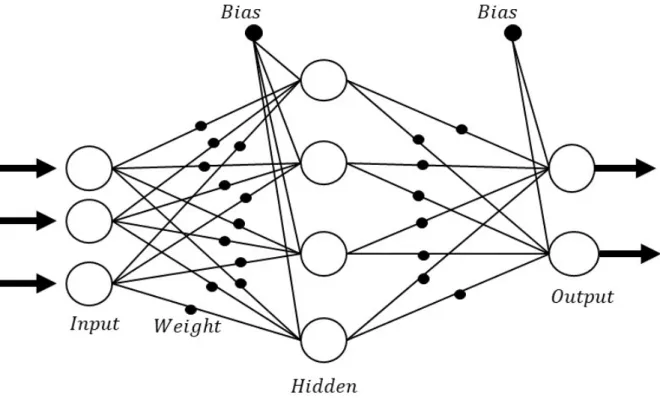
Figure 1: Feed forward network

Each neuron is fully connected and feed forward, i.e. there is no cycle within the network [36]. Every neuron is connected to the neuron in the next layer with weights, and through the activation function, the output is generated as in Fig 1. Here, the difference between the output and the real value is defined as the loss function or cost function, and this function is updated to the input through partial differentiation which is the backpropagation. For nth input, the output value is calculated to bef(Pn

i=1xiwi+b)wherexis the input,wis the weight, andbis

the bias. Here, f is the corresponding activation function, which is normally ReLU or Sigmoid function, i.e. f(x) =    0, for x <0 x, for x≥0 (ReLU) f(x) = 1 1 +e−x (Sigmoid)

The difference between the output and the target value is defined to be loss function or cost function E = 1₂Pn

(17)

and t is the target value. The error is updated to the initial weight to optimize the parameter with appropriate learning rate. The most basic optimizing algorithm is gradient descent i.e.

w=w−γ∂E_∂w. Here, the partial derivative is calculated using chain rule.

∂E ∂wji = ∂E ∂oj ∂oj ∂yj ∂yj ∂wji (8)

where yi refers to the output value before the activation function and wji refers to the

weight connecting the node from the previous layer to the node in the current node. Each partial derivative term is calculated to be

∂E ∂oj = ∂ 1 2(tj−oj) 2 ∂oj =−(tj−oj) (9) ∂oj ∂yj = ∂(1 +e −yj₎−1 ∂yj = e −yj 1 +e−yj =oi(1−oi) (10) ∂yj ∂wji = ∂wjioj ∂wji =oi (11) ∂E ∂wji =−(tj−oj)oj(1−oj)oj (12)

This updating process starts from the output node to the input node, which is the reverse direction of the feed forward process. Due to this reverse property, the process is called back-propagation. In this paper, other methods were used because despite the intuitive structure of gradient descent, it takes too much time to optimize the parameters. The other optimizers used for the research include Adagrad, Adadelta and Adam.

Gn+1 =Gn+ (∇wE(wn))2 wn+1 =wn− γ √ Gn+1+ · ∇wE(wn) (Adagrad) wn+1=wn−∆w ∆w = √ s+ √ G+· ∇wE(wn) sn+1=ηsn+ (1−η)∆w Gn+1=ηGn+ (1−η)(∇wE(wn))2 (Adadelta) vn=ηvn−1−γ∇wE(wn) wn+1 =wn−vn (momentum)

(18)

mn=β1mn−1+ (1−β1)∇wE(wn) vn=β2vn−1+ (1−β2)(∇wE(wn))2 ˆ mn= mn 1−β1t ˆ vn= vn 1−β2t wn+1 =wn− γ √ ˆ vn+ ˆ mn (Adam)

The Adagrad, which is shorten for adaptive gradient, has changing learning rate from the valueGn. Specifically, the termγ stands for the learning rate and unlike gradient descent, the

learning rate change according to Gn. Assume there is k number of parameter in wn, Gn is a

vector which hasklength. From the dot product, corresponding value inGnvector is multipied

on the gradient of the error function ∇E(wn). Hence, different learning rate can be applied to

the error function whereas same learning rate were applied in the simple gradient descent. Here,

exists so the learning rate not divided by Gn = 0. As stated in the learning step form, the Gn value is in the denominator and this make adaptive gradient. For element that has been

changed a lot, small learning rate is applied and vice versa. Due to this property, the Adagrad can make more careful optimization. However, the learning rate in Adagrad can be too small so no learning can be proceeded. As the gradient of error function get accumulated,Gnget high and

there would be no learning. To prevent this, some decaying constant η is introduced to restrict the very highGn. Theηis between 0 and 1 and this makes theGnnot too high. In the updating

process, instead of usingGn, the change ofwis applied so the hypothetical unit for the updating

equation be the same. Here, the term swas introduced for the unit change. Both the Adagrad and Adadelta developed for applying different learning rate to parameter. The Adam optimizer incorporate the advantage of momentum optimizer. In momentum, η is the momentum term to restrict the step size [37]. Specifically, vt has previous moving information and can be written

as vn = γ∇wE(wn) +ηγ∇wE(wn−1) +η2γ∇wE(wn−2) +· · ·. In Adam, mt has similar form

and has the property of momentum, and vt has similar form to Adadelta and can do adaptive

learning. Here, the hat terms normalize the mt and vt. In practise, β1 is around 0.9 and β2 is

around0.9999. Hence for the first step where there is nomt−1 orvt−1 value, the value ofmt will

be too much compare tovt. To normalize this, hat form is used so the mt first step is not too

much influential [31].

In literature, deep learning is widely used in the classification purpose where identifying the natural language data is essential. Serban et al. used deep learning to detect influenza-like-illness (ILI) outbreak from Twitter data, and Khatua et al. used Word2Vec for classifying unstructured text data to specify Zika and Ebola outbreak [38] [39]. The first attempt to predict epidemic using deep learning was made in 2005, where the number of SARS(severe acute respiratory syndrome)

(19)

patients in Shanxi was predicted with simple backpropagation neural network (BPNN) [40]. Yomwan et al. used BPNN and simple multilayer perceptron to predict the outbreak of water-borne disease (diarrhoea) in Ayutthaya province using dissolved oxygen and population density data during flood duration [41]. Xu et al. predicted the number of ILI outpatients in Hong Kong clinic using Google search data and feedforward neural network (FNN) [42]. Xue et al. merged Google Flu Trend data and Center for Disease Control (CDC) data for BPNN based epidemic prediction where the weight and threshold of BPNN are estimated using Genetic algorithm [43]. Hu et al. applied artificial tree algorithm on BPNN to develop Improved Artifical Tree BPNN (IAT BPNN) which optimizes the initial parameter of the BPNN, and compared the perfor-mance with other methods such as ANN or BPNN [44]. This methodology is also applied to animal disease: Dharmawardana et al. used basic ANN for prediction of dengue fever and Kim et al. used DNN to predict H5N1 prediction [45] [46]. The combination of traditional statistical method and deep learning is also researched by many scientists. Chakraborty et al. proposed the combination of ARIMA and neural network autoregressive (NNAR) model, which can capture both linearity and nonlinearity in the data set, for prediction of dengue cases in dengue endemic regions [47]. Soliman et al. used a Bayesian model averaging to combine FNN with ARIMA, beta regression or least absolute shrinkage and selection operators (LASSO) [48]. Some papers compared the dengue prediction performance of DNN and Recurrent Neural Network (RNN): Sathler used MLP, Long-Short Term Memory (LSTM) and Gated Recurrent Unit (GRU) to predict the dengue fever using climate features dengue data [49] and Baquero et al. compared the performance of ARIMA, ANN, LSTM and naive model in prediction of dengue [50]. Chae et al. used search query data and the Korea Center for Disease Control (KCDC) data to predict chickenpox, scarlet fever and malaria cases by using DNN and LSTM [51]. The details of RNN will be discussed in the following subsection.

2.1 Recurrent Neural Network (RNN)

The main difference between RNN and DNN is the recurrent structure as the name states. In contrast to the DNN in which each data is treated independently, the RNN employs the combination of current input, and previous data and the corresponding output proceeds to the next input. Since the spread of the disease is also affected by the cumulative cases, the RNN is widely employed in epidemiology literature.

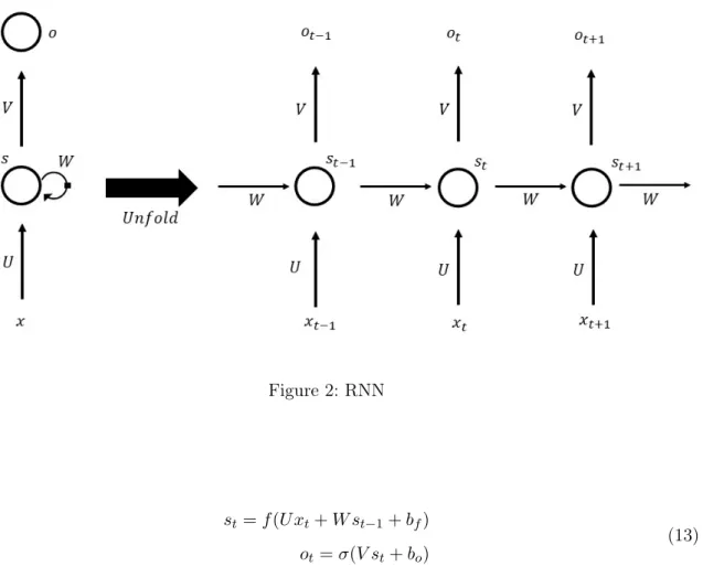
Figure 2 represents the basic structure of RNN of folded (left) and time-respected unfolded (right) diagram where xt represents the input at time t, st the hidden state at time t, ot the

output at timet, and the matrices U, V, W the same parameters used in each time step. Unlike feed forwarded DNN, the RNN has two input and output: the time tvalue input and t hidden state input, and the corresponding outputs. Here, the same valued parameters reduce the number of parameters to be learnt. In conventional vanilla RNN, the hidden state and output can be represented as

(20)

Figure 2: RNN

st=f(U xt+W st−1+bf) ot=σ(V st+bo)

(13)

whereσ andf represent the activation function andbf andborepresent the bias. Palao et al.

used RNN to predict endemic in all over the Mumbai region and made surveillance system [52]. The conventional RNN, however, has a problem for long term calculation as the bias get accu-mulated, making the computation inaccurate as the new input is shaded by previously stacked information. These standard RNN can learn the short term dependency but not the long term dependency due to gradient vanishing during backpropagation through time. To compensate for the problem, variants of RNN depending on the cell types are introduced: LSTM [53] and GRU [54].

Long Short Term Memory (LSTM)

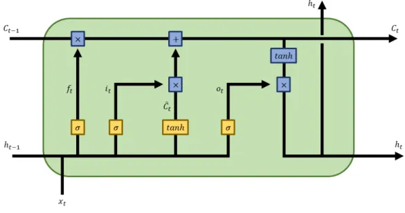
When there is a large time gap between the previous input data and provided input, there occurs the vanishing gradient problem. The LSTM solve this problem by introducing gates which can selectively value the input information. Unlike the vanilla RNN, the LSTM has two kinds of states; the hidden state learns the short term information and cell state learn the long term information. This information is controlled by the gates; the input gate decide how much to consider from cell stateCt; the forget gate how much to forget from cell state Ct−1; the output

(21)

Figure 3: LSTM

The ht represents the hidden state; theCt the cell state; the C˜t the candidate of cell state;

the it the input gate; the ft the forget gate; the ot the output gate; the xt the input; the σ

the sigmoid activation function. In forget gate, sigmoid activation is performed with inputht−1

and xt, remaining the value for output 1 and discarding the value for output 0. Next is to

decide whether to save the new data into cell state. Firstly, the input gate computeit value by

computing sigmoid ofht−1andxt. Secondly,tanhcomputes theC˜twithht−1 andxtinputs. The

next step is to renew the previous Ct−1 state with Ct. After deciding how much C−t should

be left with forget gate, the computation of input gate andC˜tis added to make new Ct. Lastly,

theht−1 and xt are computed with sigmoid andtanhactivation function consequently to make

outputht. it=σ(Wiht−1+Wixt) ft=σ(Wfht−1+Wfxt) ot=σ(Woht−1+Woxt) ˜ Ct=tanh(Wcht−1+Wcxt) Ct=ftCt−1+itC˜t ht=ottanh(Ct) (14)

The performance of the LSTM supersedes that of the RNN in terms of their prediction power. Fu et al. compared the prediction quality of the RNN and LSTM for influenza prediction [55]

(22)

and Wang et al. applied both techniques on HIV prediction in Guangxi, resulting in the best performance on LSTM when compared to RNN or ARIMA [56]. Volkova et al., to our best knowledge, firstly employed the LSTM to predict ILI dynamics using the various linguistic signals extracted from social media, suggesting that the communication behaviour is powerful in prediction and can be used for neural network model learning where ILI historical data is unavailable [57]. The LSTM shows good predictive performance in various diseases such as typhoid fever, hemorrhagic fever, mumps, conjunctivitis [58] and hand-foot-mouth disease [59], and shows improved performance when combined with a genetic algorithm to generate the initial parameter [60]. Venna et al. performed the LSTM for influenza, considering the climate factor using the time-delayed association analysis between the time series of weather and flu count, and geographical proximity by computing the spatio-temporal adjustment factor from averaging the flu variation at nearby data nodes [61]. To overcome the data sparsity problem, Wang et al. used a multi-agent system on a coarse ILI data to synthesize epidemic data and performed the LSTM to achieve accuracy in high-resolution forecasting [62].

Gated Recurrent Unit (GRU)

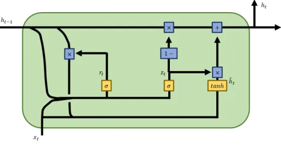
The GRU is developed to reduced the parameter and computation time of the LSTM. The main difference is that the GRU combines forget gate and input gate into a single update gate, hence achieving a simpler structure.

Figure 4: GRU

(23)

con-trolling the portion of previously hidden state output. The reset gate rt readjust the previous

memory to forge a new memory. Thus, the memory candidateh˜t consists of current input and

previous memory, where the memory is reset when rt = 0 and used when rt = 1. The GRU is

capable of capturing long term sequence data and has lower memory capacity.

zt=σ(Wzht−1+Wzxt) rt=σ(Wrht−1+Wrxt) ˜ ht=tanh(W rtht−1+W xt) ht= (1−zt)ht−1+zth˜t (15)

The GRU method, however, is little in its application on the epidemiology. Livelo et al. used the GRU for classifying dengue tweet [63] and Sathler et al. compared the GRU with other neural networks such as MLP and LSTM in their dengue prediction power, resulting in best performance for GRU [49].

2.2 Convolutional Neural Network (CNN)

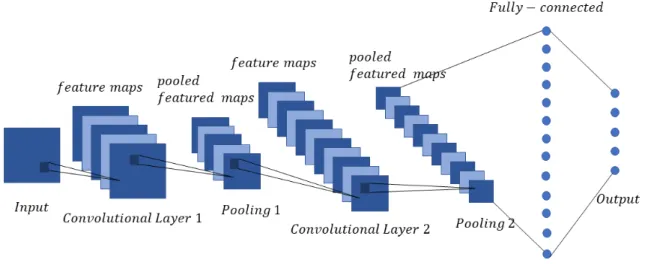
The CNN is an algorithm mainly used to capture the image or spatial information. Unlike the DNN or RNN, the CNN uses dimensional data as input value and results in three-dimensional information as an output. This aspect enables the algorithm to maintain the spatial features. Here, the term convolution refers to the integral of the multiplication of two functions where one is reflected. Whereas the MLP connects all weights on a single node, the weights are connected only to the neighbouring nodes. This local connection of the same filter reduces the number of parameters and computational speed. Furthermore, since the CNN processes one image into multiple pieces of small neighbouring image segments, the distortion or translation of the image can be captured. Most of the CNNs used for today’s research have their base on the model proposed by Yann Lecun, where he used backpropagation to learn the filter coefficient from the handwritten number [64]. His model mainly consists of three-layer: convolutional layer conducts convolution computation to extracts the meaningful feature map; pooling layer reduces the number of feature by sub-sampling; fully connected layer connects all nodes and acts like normal ANN.

In convolutional layer, a kernel of smaller size and same depth is applied to the entire image. The kernel, also known as the window, strides the image and calculates the inner product, learning the pattern and local information by amplifying the feature signal and suppressing the noise. The result after applying the same window and bias is called feature map, and the set of feature maps is the convolutional layer. Depend on the stride size, the boundary part of

(24)

Figure 5: CNN

the input data can be removed. Padding is applied to prevent the lose and to ensure the same dimensionality of output and input. The size of the output follows equation (16).

(Oh, Ow) = (

h+ 2P−Fh S + 1,

w+ 2P −Fw

S + 1) (16)

where Oh refers the height of output, Ow width of output,Fh height of filter,Fw width of

filter, h height of input, w width of input, P size of padding, S size of stride. Mostly, the sizes of convolutional layer and input data are controlled to have the same dimension and the dimensionality reduction occurs in the following pooling layer.

Pooling is the process of attaining a single value from the selected size window. Depend on types of the data, different types of pooling are used. For example, average pooling is used for the smoothing of the image, and max pooling is used for sharping the image, which fits for MNIST data where the contrast of background and the handwriting is important. This reduction of parameters is also helpful for the prevention of overfitting. After alternatively applying the convolutional and pooling layer, the extracted features are connected to a fully connected layer, controlling the number of feature.

As well as for the visual image, the CNN is also used for processing the sequence data due to its ability that captures the entire sequence and speed. Zhong et al. first used the CNN to predict the influenza dynamics by capturing the disease flow in location network and see how the attributes of locations affect the prediction accuracy [65]. Andersson et al. used Google Street View data to extract useful feature for prediction of the dengue fever and Rehman et al. used satellite data to extract landscape features and incorporated them into the SIR model [66] [67].

(25)

Some researchers used the CNN to extract sequence data, where Molaei et al. used the CNN to extract Twitter data to predict ILI and Bu et al. used Python web crawler to extract web search data and predicted flu [68] [69]. As well as extracting the sequence data, Gencoglu et al. used the CNN to capture illness-related picture such as drug photo from Instagram and predicted flu [70]. Among several CNN model, residual network (ResNet) model is used in accordance with RNN to capture the spatial feature of the epidemics. ResNet enables the CNN to have more convolutional layers by applying bottleneck structure to prevent gradient vanishing problem causing from many hidden layers. This bottleneck makes skip connection between input and output whereby accelerates the learning speed by providing learning object and mitigates the overfitting problem, yielding more accurate prediction. Xi et al. used ResNet to predict the influenza trend and compared the root mean square error (RMSE) with several methods including the ANN or LSTM, attaining the best result for ResNet [71]. Wu et al. combined GRU and ResNet to capture both the temporal and spatial features of the ILI in Japan and the United States, giving out best when compared to Gaussian Process or vector autoregression [2].

Graph Convolutional Network (GCN)

Some data such as social, information or road can be represented as a graph using network science. With graph representation, the meaningful connection can be made easier than the image which merely reflects the Euclidean distances. Although spatial CNN performs well under the conditions including grid structure and translational invariance, it is hard to perform learning for non-Euclidean data. The Graph Convolutional Network (GCN) constructs network within the data set and use as input, hence changing the spatial domain data into spectral domain [72]. The graph can be represented asG= (V, E)whereV represents the set of vertices or nodes and

E the set of edges or relationships. The vertices may imply the constituent of the system such as individual or region, and the edges may imply the relationship or interaction of the nodes such as connection or linkage. Among the many types of graph, this paper focuses on the simplest form, unweighted and undirectional graph.

(26)

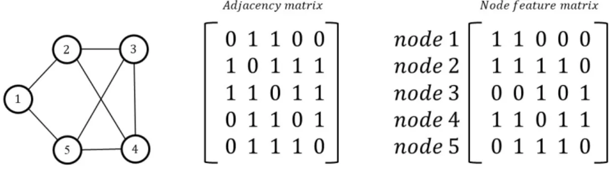
Fig. 6 shows an example of a graph and its relevant matrix where the adjacency matrix is

AN×N and feature matrix isXN×F. Here,N represents the number of nodes where in this case is 5 and F represents the number of features where in this case is 5. The adjacency matrix is symmetric pairwise distance matrix with element values are either 1 or 0, where 1 represents a connection and 0 no connection. To update the node history, the identity matrix is summed to the adjacency matrix to change the diagonal values to 1. For the case of a weighted graph, a similarity matrix of an element between 0 and 1 is used instead of the adjacency matrix.

As the name stated, the GCN conducts convolutional computation and update the values of the features of the nodes while the shape of the graph remains unchanged. A single hidden layer of graph receives first order neighbourhood information by multiplying the adjacency matrix and feature matrix, and as the layer stacks up, the node can receive information from multiple order of neighbouring nodes. By controlling the number of layers, the information travel distance can be regulated. In Graph Neural Network (GNN), the original model of GCN, the embedding of the new node is made by the sum of aggregated neighbouring nodes and concatenated the original node itself. Unlike the GNN which use different aggregate and concatenate function and weight, the GCN use the same weight for the node and the neighbouring nodes. To even the effect of each node, Laplacian normalization is applied to the propagation.

Hi(l+1) =σ( X j∈N(i) Hj(l)W(l)+b(l)) (17) H(l+1) =σ(AH(l)W(l)+b(l)) (18) H(l+1)=σ(D−12ADˆ − 1 2H(l)W(l)+b(l)) (19)

Equation (17) represents the recursive computation of how the lth neighborhood nodes are updated tol+ 1th layer where Hi(l+1) represents the hidden state inl+ 1 layer and ith node, W(l) the weight matrix, b(l) the bias vector and σ the activation function. Instead of using for loop, the adjacency matrix is used for simplification in equation (18). Since the adjacency matrix

A is not normalized, it can change the scale of the feature vector. By adding degree matrix D

which refers to the number of connection attached to each node, and by adding identity matrix to adjacency matrix, A+I = ˆA, equation (19) is obtained. This GCN model can both capture the computational efficiency through weight sharing and graph local feature [73]. With all the advantage of the GCN which can capture meaningful information for non-Euclidean distance, it has not been explored in epidemiology literature to the best knowledge.

(27)

2.3 Graph Convolutional Network Gated Recurrent Unit (GCNGRU)

A combination of the GCN and GRU, both of which are unexplored in epidemiology literature, is used for the research. Compare to the other RNN mechanism such as LSTM, GRU requires less parameter and hence reducing the computation time and overfitting risk. Hence, the GRU was chosen for the temporal investigation of this research. Also, the GCN was chosen for the research since the CNN was initially developed to learn images or grid data, which is not useful for non-Euclidean distance such as the United States traffic network which directly affects the spread of disease. Furthermore, the GCN can be more suitable for capturing the disease spread since the disease can only be transmitted to the isolated area such as island by aeroplane or shipment. For this case, the epidemic relationship between the island and major city will be stronger than the island and its neighbouring region. Also, the GCN can be further accurate by introducing Attention GCN which has different weight depending on the connection importance. In this aspect, this paper chooses the combination model GCNGRU to forecast the epidemics.

zt=σ(Wz[Hl, ht−1] +bz) rt=σ(Wr[Hl, ht−1] +br) ˜ ht=tanh(Wht[H l_{, r} tht−1] +bht) ht= (1−zt)ht−1+zth˜t (20)

Equation (20) shows the GCNGRU model which is used for the research. The data from the GCN cell goes to GRU cell and performs prediction. The model will be evaluated via multiple metric and compared with previous research which employed ResNet + GRU.

Similar method was used on research out of epidemiology literature. Cui et al. combined GCN and LSTM to make traffic graph convolutional long short term memory neural network (TGC-LSTM) to track the traffic on the road [74]. Zhao et al. proposed T-GCN model, which is composed of GCN and GRU, and used traffic speed data in Shenzan and Los Angeles to predict the traffic under different time horizon [75]. As the investigation of time varying influenza rate in each region resembles the time varying traffic in each road segment, the experiment was done with the United States influenza rate time series data for multiple U.S. regions.

(28)

III

Experiment

3.1 Data Description

For the empirical evaluation of the model, a real world ILI activity level data in the United States were chosen. The data were collected by the U.S. Outpatient Influenza-like Illness Surveillance Network (ILINet) which is consists of around 30 million patient visit data gained from more than 2900 healthcare providers in the 50 states, District of Columbia and New York city. Here, the standard for ILI is defined as fever of higher than 37.8◦C and a cough or sore throat. The activity levels represents the comparison of the percent of outpatients reported in a jurisdiction due to ILI and the percent of outpatients when there is no report of influenza virus circulation for two or more consecutive weeks. To take into account the geographical and temporal difference, the baselines for each states and each time period were set differently. The ILI activity level map is shown below.

Figure 7: ILI Activity map [1]

The activity is divided into 10 levels which correspond to the positive and negative standard deviation to baseline. As in the map, the activity level is represented by colour where the green represents activity level 1 which is below the mean, and the red represents 10 which corresponds to 8 or more standard deviation. The data does not contain information about the extent of spread of ILI within a state and may poorly represents certain populations within a state [76]. After removing the states that have insufficient data, for example the District of Columbia in Figure 7, 2009 to 2016 weekly ILI activity level data of 29 states data out of 52 region

(29)

were selected for the empirical evaluation. In practise, the table from ILI activity map and the adjacency matrix which contain neighbouring information was used.

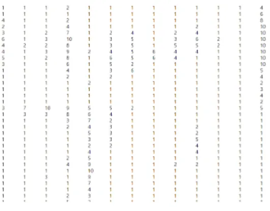
(a) ILI activity level weekly table (b) Neighbouring adjacency matrix

Figure 8: Data used for the evaluation [2]

Figure 8 (a) is the ILI activity level weekly data where the horizontal axis is the week and vertical axis is each states. Figure 8 (b) is the adjacency matrix using neighbouring information where 0 denotes no connection and 1 denoted neighbouring relation.

3.2 Evaluation metrics

This paper adopted two evaluation metrics: root mean square error (RMSE) was used to measure the prediction error where the smaller value represents more accurate prediction: Pearson’s corre-lation coefficient (CORR) to measure the linear correcorre-lation between the ture and the prediction. When the prediction is denoted to beyˆi and and the trueyi, the metrics are

RM SE = s 1 n X i (ˆyi−yi)2 CORR= P i(ˆyi−mean(ˆy))(yi−mean(y)) pP i(ˆyi−mean(ˆy))2pPi(yi−mean(y))2

(30)

IV

Result

The aim of this evaluation is to check the performance of the GCNGRU model by comparing to the existing model, CNNRNN-res, which is suggested by Wu et al. [2]. As introduced in the last of 2.2 CNNsection, the CNNRNN-res is a combination of the ResNet (CNN) and GRU (RNN). Among many deep learning applied epidemic model, this particular model was chosen for two reasons. First, to the best knowledge, the CNNRNN-res is the first and only model which captures both the spatial and temporal features of the data by deep learning methodologies. Next, the model shows dominating performance when compared to the other statistical model including global autoregression (GAR), autoregression (AR), vector autoregression (VAR), and gaussian process (GP). For the comparison, exactly same data and the same number of epoch have been applied to the GCNGRU. To achieve the optimal value, multiple parameters have been applied as well.

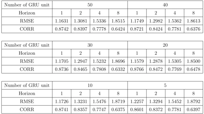
Number of GRU unit 50 40

Horizon 1 2 4 8 1 2 4 8

RMSE 1.1631 1.3081 1.5336 1.8515 1.1749 1.2982 1.5362 1.8613 CORR 0.8742 0.8397 0.7778 0.6424 0.8721 0.8424 0.7781 0.6376

Horizon 1 2 4 8 1 2 4 8

RMSE 1.1705 1.2947 1.5232 1.8696 1.1579 1.2878 1.5305 1.8500 CORR 0.8736 0.8465 0.7808 0.6332 0.8766 0.8472 0.7769 0.6478

Horizon 1 2 4 8 1 2 4 8

RMSE 1.1726 1.3231 1.5476 1.8719 1.2257 1.3294 1.5452 1.8792 CORR 0.8741 0.8357 0.7747 0.6375 0.8601 0.8372 0.7781 0.6397

Table 1: RMSE and CORR for the various number of RNN units

Table 1 was reproduced with controlled parameters: the Adam optimizer, 2000 number of epochs which is the same number to the result from CNNRNN-res, the batch size of 32, and the learning rate of 0.001. For all experiments conducted for this paper, the epoch refers to the number of iterative computation for the entire set of data. For example, one epoch is when the entire data is passed forward and backward through the model only once. In the table, the horizon represents the time step of prediction. For example, the 1 value of horizon represents the prediction horizons of 1 week which is the time step of the original data. Here, the varied

(31)

parameter ’Number of GRU unit’ refers to the dimensionality or length of the hidden state of the GRU cell. The evaluation resulted in consistent fair performance for every experiment, where the best output gained from 20 number of GRU units. This value judges the capability of the GRU cell capturing the structural and semantic features of the input data. Normally, a large number of RNN unit make better output but if the number of units exceeds a certain number, the model gets over complexed and the computational difficulty makes bad performance.

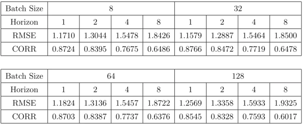
Batch Size 8 32 Horizon 1 2 4 8 1 2 4 8 RMSE 1.1710 1.3044 1.5478 1.8426 1.1579 1.2887 1.5464 1.8500 CORR 0.8724 0.8395 0.7675 0.6486 0.8766 0.8472 0.7719 0.6478 Batch Size 64 128 Horizon 1 2 4 8 1 2 4 8 RMSE 1.1824 1.3136 1.5457 1.8722 1.2569 1.3358 1.5933 1.9325 CORR 0.8703 0.8387 0.7737 0.6376 0.8545 0.8328 0.7593 0.6017

Table 2: RMSE and CORR for various number of batch size

With 20 number of GRU units and other controlled parameters, the batch size has been varied. The result in table 2 shows that the batch size of 32 yields the best result. The batch size refers to the total number of training samples in a single batch. For the mini-batch optimization, the batch size is between 1 and the size of the training set. For example, training data with 320 sample has 10 batches for 32 sized batch. Since the epoch is 2000, there will be total

10×2000 = 20000steps of update(learning). When the batch size is large, the model will learn many data at once and the training process will be faster. The computer memory capacity, however, is limited, too large batch size may lead to poor learning performance.

Introduced in equation (7), the learning rate is the step size of learning between 0 and 1, where 0 is no learning over the iteration and 1 is the perfect learning where the parameter should be updated to the optimal from just single iteration. Normally, a large value of learning rate leads to overshooting, which means the step is too big to find the detailed optimal. When the learning rate is too small, it will take too much computation time to find the optimal and the learning may fall into local minima. For this experiment, 0.001 value of the learning rate was found to be the optimal hyperparameter.

(32)

Learning Rate 1 0.1 Horizon 1 2 4 8 1 2 4 8 RMSE 1.3228 1.9403 2.0681 2.3946 1.1769 1.2908 1.5437 1.8309 CORR 0.8396 0.6879 0.5136 0.3835 0.8709 0.8427 0.7719 0.6541 Learning Rate 0.01 0.001 Horizon 1 2 4 8 1 2 4 8 RMSE 1.1728 1.2948 1.5377 1.8518 1.1579 1.2878 1.5464 1.8500 CORR 0.8718 0.8435 0.7728 0.6449 0.8766 0.8472 0.7719 0.6478 Learning Rate 0.0001 Horizon 1 2 4 8 RMSE 1.2447 1.3281 1.6076 1.9494 CORR 0.8566 0.8364 0.7519 0.5970

Table 3: RMSE and CORR for various learning rate

As mentioned at the beginning of the model section, this paper used other kinds of optimizer other than gradient descent as the gradient descent need to calculate loss function for each step, leading to a huge amount of computational cost. Specifically, Adagrad, Adadelta and Adam were used to evaluate the model. The Adagrad optimizer applies different learning rate to parameters and Adadelta is the extension of Adagrad which corrected the vanishing step size problem. The Adam is an incorporation of Adadelta and momentum, earning the advantage of both methods. As many literatures reported, Adam has the best value followed by Adagrad, whereas Adadelta shows poor performance. This may stem from local minima since the Adadelta optimizer cannot escape the local minima.

The optimal output was then compared with the output from the CNNRNN-res model, as shown in Table 5.

The optimal result from the experiment was compared with the result from another CN-NRNN model which used the same data [2]. The CNCN-NRNN-res is the only model that captured both the spatial and temporal feature using Deep Learning in epidemiology. The CNNRNN-res model was compared with various other statistical methods such as vector autoregression or Gaussian process, and earned the best result. From the comparison, it is shown in the table that the suggested GCNGRU model achieved better metric value for all range of horizon. Com-paring the two models, GCNGRU showed 1.6%, 3.9%, 6.1%, 5.0% improvement in 1, 2, 4 and 8 predictions of horizon respectively for RMSE when considering the ILI activity level scale, and showed 3.7%, 7.7%, 10.8%, 10.9% improvement for CORR respectively. Especially for long

(33)

Optimizer Adam Adagrad Horizon 1 2 4 8 1 2 4 8 RMSE 1.1579 1.2878 1.5464 1.8500 1.2815 1.5733 1.9036 2.1857 CORR 0.8766 0.8472 0.7719 0.6478 0.8487 0.7636 0.6217 0.4414 Optimizer Adadelta Horizon 1 2 4 8 RMSE 6.2471 3.8066 4.2754 4.6189 CORR -0.3057 -0.2939 -0.7905 -0.6718

Table 4: RMSE and CORR for a various optimizer

US Region Horizon Method Metiric 1 2 4 8 CNNRNN-res RMSE 1.3147 1.6783 2.1613 2.3465 CORR 0.8033 0.6942 0.5564 0.4298 GCNGRU RMSE 1.1579 1.2878 1.5464 1.8500 CORR 0.8766 0.8472 0.7719 0.6478

Table 5: CNNRNN-res vs GCNGRU

term prediction, the GCNGRU showed better performance overall. Figure 8 and 9 shows the training graph in terms of RMSE and CORR change. Without a spike, the learning processed well. Figure 10 depicts the visualisation of the prediction for the sample four states. For all 4 graphs, the prediction (red line) shows good accordance to the true (blue line)

(34)

Figure 9: RMSE change for train and test

(35)

(a)

(b)

(c)

(d)

(36)

V

Conclusion

In this paper, Deep Learning method for forecasting the epidemics has introduced. Though it is a relatively new method, Deep Learning showed fair performance in epidemiological prediction and developed by many researchers. As a challenging problem, a combination of GCN and GRU model was applied to ILI activity level data. The evaluation showed consistent and good performance throughout the experiment and better performance when compared to the existing model. Many aspects of Deep Learning, however, is unknown and it is hard to certain that the proposed model will show good performance on other epidemic data. For future research, the same model should be applied to other kinds of disease and should be checked whether the model shows consistently good result. Furthermore, this model can be developed by applying traffic adjacency matrix rather than a neighbouring matrix. As the spread of disease is mainly due to the contact, it is probable that traffic matrix can predict the spread of epidemics better than the neighbouring matrix. Also, the model can be further developed by introducing directionality to the graph. For example, the conveyance of livestock can be directional. Adjustment in the hyperparameter also may improve the model.

(37)

References

[1] “2015-16 influenza season week 8 ending feb 27, 2016,” https://gis.cdc.gov/grasp/fluview/ main.html#a8.

[2] Y. Wu, Y. Yang, H. Nishiura, and M. Saitoh, “Deep learning for epidemiological predic-tions,” in The 41st International ACM SIGIR Conference on Research & Development in

Information Retrieval. ACM, 2018, pp. 1085–1088.

[3] “Epidemiology,” https://www.who.int/topics/epidemiology/en/.

[4] “From panic and neglect to investing in health security: Financing pandemic prepared-ness at a national level,” https://www.worldbank.org/en/topic/pandemics/publication/

from-panic-neglect-to-investing-in-health-security-financing-pandemic-preparedness-at-a-national-level.

[5] D. Earn, F. Brauer, P. van den Driessche, and J. Wu,Mathematical epidemiology. Springer Berlin, 2008.

[6] “Si and sis models,” https://institutefordiseasemodeling.github.io/Documentation/general/ model-si.html.

[7] S.-G. Lee, R.-Y. Ko, and J.-H. Lee, “Mathematical modelling of the h1n1 influenza,”

Com-munications of Mathematical Education, vol. 24, no. 4, pp. 877–889, 2010.

[8] F. Brauer, “Some simple epidemic models,” Mathematical Biosciences and Engineering, vol. 3, no. 1, p. 1, 2006.

[9] S. Ryu and B. Choi, “Development of epidemic model using the stochastic method,” Journal

of the Korean Data and Information Science Society, vol. 26, no. 2, pp. 301–312, 2015.

[10] T. Britton and P. D. O’NEILL, “Bayesian inference for stochastic epidemics in populations with random social structure,” Scandinavian Journal of Statistics, vol. 29, no. 3, pp. 375– 390, 2002.

[11] G. Streftaris and G. J. Gibson, “Bayesian inference for stochastic epidemics in closed pop-ulations,” Statistical Modelling, vol. 4, no. 1, pp. 63–75, 2004.

[12] Z.-X. Wu and H.-F. Zhang, “Peer pressure is a double-edged sword in vaccination dynamics,”

(38)

[13] 심은하, “외국의 감염병 발생 예측 및 확산모형 사례,” HIRA 정책동향, vol. 10, no. 5, pp. 25–28, 2016.

[14] A. Weigend and N. Gershenfeld, “The future of time series,” in Proceedings of the NATO

advanced Research Workshop on Comparative Time Series Analysis. Citeseer, 1992, pp.

1–70.

[15] G. Udny Yule, “On a method of investigating periodicities in disturbed series, with special reference to wolfer’s sunspot numbers,” Philosophical Transactions of the Royal Society of London Series A, vol. 226, pp. 267–298, 1927.

[16] E. Slutzky, “The summation of random causes as the source of cyclic processes,” Economet-rica: Journal of the Econometric Society, pp. 105–146, 1937.

[17] P. Whittle, “The analysis of multiple stationary time series,” Journal of the Royal Statistical Society: Series B (Methodological), vol. 15, no. 1, pp. 125–139, 1953.

[18] G. E. Box, G. M. Jenkins, and G. Reinsel, “Time series analysis: forecasting and con-trol holden-day san francisco,” BoxTime Series Analysis: Forecasting and Control Holden Day1970, 1970.

[19] “The box-jenkins method,” https://ncss-wpengine.netdna-ssl.com/wp-content/themes/ ncss/pdf/Procedures/NCSS/The_Box-Jenkins_Method.pdf.

[20] C. A. Sims, “Macroeconomics and reality,” Econometrica: journal of the Econometric Soci-ety, pp. 1–48, 1980.

[21] N. S. Altman, “An introduction to kernel and nearest-neighbor nonparametric regression,”

The American Statistician, vol. 46, no. 3, pp. 175–185, 1992.

[22] C. Cortes and V. Vapnik, “Support-vector networks,” Machine learning, vol. 20, no. 3, pp. 273–297, 1995.

[23] W. S. McCulloch and W. Pitts, “A logical calculus of the ideas immanent in nervous activ-ity,” The bulletin of mathematical biophysics, vol. 5, no. 4, pp. 115–133, 1943.

[24] F. Rosenblatt,The perceptron, a perceiving and recognizing automaton Project Para. Cor-nell Aeronautical Laboratory, 1957.

[25] M. Minsky and S. Papert, “An introduction to computational geometry,” Cambridge tiass., HIT, 1969.

[26] T. Kohonen, “Self-organized formation of topologically correct feature maps,” Biological cybernetics, vol. 43, no. 1, pp. 59–69, 1982.

[27] P. J. Werbos,The roots of backpropagation: from ordered derivatives to neural networks and political forecasting. John Wiley & Sons, 1994, vol. 1.

(39)

[28] J. J. Hopfield, “Neural networks and physical systems with emergent collective computa-tional abilities,” Proceedings of the national academy of sciences, vol. 79, no. 8, pp. 2554– 2558, 1982.

[29] D. E. Rumelhart, G. E. Hinton, and R. J. Williams, “Learning internal representations by error propagation,” California Univ San Diego La Jolla Inst for Cognitive Science, Tech. Rep., 1985.

[30] H. Robbins and S. Monro, “A stochastic approximation method,” The annals of mathemat-ical statistics, pp. 400–407, 1951.

[31] D. P. Kingma and J. Ba, “Adam: A method for stochastic optimization,” arXiv preprint arXiv:1412.6980, 2014.

[32] J. Duchi, E. Hazan, and Y. Singer, “Adaptive subgradient methods for online learning and stochastic optimization,” Journal of Machine Learning Research, vol. 12, no. Jul, pp. 2121– 2159, 2011.

[33] “Overview of mini batch gradient descent,” https://www.cs.toronto.edu/~tijmen/csc321/ slides/lecture_slides_lec6.pdf.

[34] V. Nair and G. E. Hinton, “Rectified linear units improve restricted boltzmann machines,”

in Proceedings of the 27th international conference on machine learning (ICML-10), 2010,

pp. 807–814.

[35] N. Srivastava, G. Hinton, A. Krizhevsky, I. Sutskever, and R. Salakhutdinov, “Dropout: a simple way to prevent neural networks from overfitting,” The journal of machine learning research, vol. 15, no. 1, pp. 1929–1958, 2014.

[36] A. Zell, Simulation neuronaler netze. Addison-Wesley Bonn, 1994, vol. 1, no. 5.3.

[37] D. E. Rumelhart, G. E. Hinton, R. J. Williams et al., “Learning representations by back-propagating errors,” Cognitive modeling, vol. 5, no. 3, p. 1, 1988.

[38] O. S,erban, N. Thapen, B. Maginnis, C. Hankin, and V. Foot, “Real-time processing of social

media with sentinel: a syndromic surveillance system incorporating deep learning for health classification,” Information Processing & Management, vol. 56, no. 3, pp. 1166–1184, 2019.

[39] A. Khatua, A. Khatua, and E. Cambria, “A tale of two epidemics: Contextual word2vec for classifying twitter streams during outbreaks,” Information Processing & Management, vol. 56, no. 1, pp. 247–257, 2019.

[40] Y. Bai and Z. Jin, “Prediction of sars epidemic by bp neural networks with online prediction strategy,” Chaos, Solitons & Fractals, vol. 26, no. 2, pp. 559–569, 2005.

(40)

[41] C. C. PEERAYOMWAN and P. RAKWATIN, “A study of waterborne diseases during flooding using radarsat-2 imagery and a back propagation neural network algorithm.”

[42] Q. Xu, Y. R. Gel, L. L. R. Ramirez, K. Nezafati, Q. Zhang, and K.-L. Tsui, “Forecasting influenza in hong kong with google search queries and statistical model fusion,” PloS one, vol. 12, no. 5, p. e0176690, 2017.

[43] H. Xue, Y. Bai, H. Hu, and H. Liang, “Influenza activity surveillance based on multiple regression model and artificial neural network,” IEEE Access, vol. 6, pp. 563–575, 2017.

[44] H. Hu, H. Wang, F. Wang, D. Langley, A. Avram, and M. Liu, “Prediction of influenza-like illness based on the improved artificial tree algorithm and artificial neural network,”

Scientific reports, vol. 8, no. 1, p. 4895, 2018.

[45] K. Dharmawardana, K. Lokuge, P. Dassanayake, M. Sirisena, L. Fernando, A. S. Perera, and S. Lokanathan, “Annex 19: predictive model for the dengue incidences in sri lanka using mobile network big data.” 2018.

[46] 김성현, 최준기, 김재석, 장아름, 이재호, 차경진, and 이상원, “빅데이터와 딥러닝을 활용한 동물감염병확산차단,” 지능정보연구, vol. 24, no. 4, pp. 137–154, 2018.

[47] T. Chakraborty, S. Chattopadhyay, and I. Ghosh, “Forecasting dengue epidemics using a hybrid methodology,” Physica A: Statistical Mechanics and its Applications, vol. 527, p. 121266, 2019.

[48] M. Soliman, V. Lyubchich, and Y. R. Gel, “Complementing the power of deep learning with statistical model fusion: Probabilistic forecasting of influenza in dallas county, texas, usa,”

Epidemics, p. 100345, 2019.

[49] C. Sathler and J. Luciano, “Predictive modeling of dengue fever epidemics: A neural network approach,” 2017.

[50] O. S. Baquero, L. M. R. Santana, and F. Chiaravalloti-Neto, “Dengue forecasting in são paulo city with generalized additive models, artificial neural networks and seasonal autore-gressive integrated moving average models,” PloS one, vol. 13, no. 4, p. e0195065, 2018.

[51] S. Chae, S. Kwon, and D. Lee, “Predicting infectious disease using deep learning and big data,” International journal of environmental research and public health, vol. 15, no. 8, p. 1596, 2018.

[52] S. D. H. G. A. Y. Sagar Palao, Abhishek Shahasane, “A proposal for epidemic prediction using deep learning,” International Journal of Engineering Research in Computer Science and Engineering, vol. 4, 2017.

[53] S. Hochreiter and J. Schmidhuber, “Long short-term memory,” Neural computation, vol. 9, no. 8, pp. 1735–1780, 1997.

(41)

[54] K. Cho, B. Van Merriënboer, C. Gulcehre, D. Bahdanau, F. Bougares, H. Schwenk, and Y. Bengio, “Learning phrase representations using rnn encoder-decoder for statistical ma-chine translation,” arXiv preprint arXiv:1406.1078, 2014.

[55] B. Fu, Y. Yang, Y. Ma, J. Hao, S. Chen, S. Liu, T. Li, Z. Liao, and X. Zhu, “Attention-based recurrent multi-channel neural network for influenza epidemic prediction,” in 2018 IEEE

International Conference on Bioinformatics and Biomedicine (BIBM). IEEE, 2018, pp.

1245–1248.

[56] G. Wang, W. Wei, J. Jiang, C. Ning, H. Chen, J. Huang, B. Liang, N. Zang, Y. Liao, R. Chen et al., “Application of a long short-term memory neural network: a burgeoning method of deep learning in forecasting hiv incidence in guangxi, china,” Epidemiology & Infection, vol. 147, 2019.

[57] S. Volkova, E. Ayton, K. Porterfield, and C. D. Corley, “Forecasting influenza-like illness dy-namics for military populations using neural networks and social media,” PloS one, vol. 12, no. 12, p. e0188941, 2017.

[58] W. Jia, Y. Wan, Y. Li, K. Tan, W. Lei, Y. Hu, Z. Ma, X. Li, and G. Xie, “Integrating multiple data sources and learning models to predict infectious diseases in china,” AMIA Summits on Translational Science Proceedings, vol. 2019, p. 680, 2019.

[59] Y. Wang, C. Xu, S. Zhang, L. Yang, Z. Wang, Y. Zhu, and J. Yuan, “Development and evaluation of a deep learning approach for modeling seasonality and trends in hand-foot-mouth disease incidence in mainland china,” Scientific reports, vol. 9, no. 1, p. 8046, 2019.

[60] D. N. Pham, T. Aziz, A. Kohan, S. Nellis, J. J. Khoo, D. Lukose, S. AbuBakar, A. Sattar, H. H. Ong et al., “How to efficiently predict dengue incidence in kuala lumpur,” in 2018 Fourth International Conference on Advances in Computing, Communication & Automation

(ICACCA). IEEE, 2018, pp. 1–6.

[61] S. R. Venna, A. Tavanaei, R. N. Gottumukkala, V. V. Raghavan, A. S. Maida, and S. Nichols, “A novel data-driven model for real-time influenza forecasting,” IEEE Access, vol. 7, pp. 7691–7701, 2018.

[62] L. Wang, J. Chen, and M. Marathe, “Defsi: Deep learning based epidemic forecasting with synthetic information,” Proceedings of the 30th innovative Applications of Artificial Intelli-gence (IAAI), 2019.

[63] E. D. Livelo and C. Cheng, “Intelligent dengue infoveillance using gated recurrent neural learning and cross-label frequencies,” in 2018 IEEE International Conference on Agents

(42)

[64] Y. LeCun, B. Boser, J. S. Denker, D. Henderson, R. E. Howard, W. Hubbard, and L. D. Jackel, “Backpropagation applied to handwritten zip code recognition,”Neural computation, vol. 1, no. 4, pp. 541–551, 1989.

[65] S. Zhong and L. Bian, “Predicting influenza dynamics using a deep learning approach,” in

International Conference on GIScience Short Paper Proceedings, vol. 1, no. 1, 2016.

[66] V. O. Andersson, M. A. F. Birck, and R. M. Araujo, “Towards predicting dengue fever rates using convolutional neural networks and street-level images,” in 2018 International Joint

Conference on Neural Networks (IJCNN). IEEE, 2018, pp. 1–8.

[67] N. Abdur Rehman, U. Saif, and R. Chunara, “Deep landscape features for improving vector-borne disease prediction,” in Proceedings of the IEEE Conference on Computer Vision and

Pattern Recognition Workshops, 2019, pp. 44–51.

[68] S. Molaei, M. Khansari, H. Veisi, and M. Salehi, “Predicting the spread of influenza epi-demics by analyzing twitter messages,” Health and Technology, pp. 1–16, 2019.

[69] Y. Bu, J. Bai, Z. Chen, M. Guo, and F. Yang, “The study on china’s flu prediction model based on web search data,” Journal of Data Analysis and Information Processing, vol. 6, no. 03, p. 79, 2018.

[70] O. Gencoglu and M. Ermes, “Predicting the flu from instagram,” arXiv preprint

arXiv:1811.10949, 2018.

[71] G. Xi, L. Yin, Y. Li, and S. Mei, “A deep residual network integrating spatial-temporal properties to predict influenza trends at an intra-urban scale,” in Proceedings of the 2nd

ACM SIGSPATIAL International Workshop on AI for Geographic Knowledge Discovery.

ACM, 2018, pp. 19–28.

[72] M. Defferrard, X. Bresson, and P. Vandergheynst, “Convolutional neural networks on graphs with fast localized spectral filtering,” in Advances in neural information processing systems, 2016, pp. 3844–3852.

[73] T. N. Kipf and M. Welling, “Semi-supervised classification with graph convolutional net-works,” arXiv preprint arXiv:1609.02907, 2016.

[74] Z. Cui, K. Henrickson, R. Ke, and Y. Wang, “Traffic graph convolutional recurrent neural network: A deep learning framework for network-scale traffic learning and forecasting,”

arXiv preprint arXiv:1802.07007, 2018.

[75] L. Zhao, Y. Song, C. Zhang, Y. Liu, P. Wang, T. Lin, M. Deng, and H. Li, “T-gcn: A tem-poral graph convolutional network for traffic prediction,” IEEE Transactions on Intelligent Transportation Systems, 2019.

(43)

[76] “Overview of influenza surveillance in the united states,” https://www.cdc.gov/flu/pdf/ weekly/overview.pdf.

(44)

Acknowledgements

With the greatest respect, I would like to express my sincere appreciation to all UNIST members. I am much obliged to have the honour of being the most humble and obedient member of UNIST math society.

(45)