SYSTEMIC VALIDATION OF CONSEQUENCE-BASED RISK MANAGEMENT FOR SEISMIC REGIONAL LOSSES

(1)

SYSTEMIC VALIDATION OF CONSEQUENCE-BASED RISK

MANAGEMENT FOR SEISMIC REGIONAL LOSSES

Joshua S. Steelman and Jerome F. Hajjar

A Report of the Mid-America Earthquake Center

Mid-America Earthquake Center

1241 Newmark Civil Engineering Laboratory

205 North Mathews Avenue

University of Illinois at Urbana-Champaign

Urbana, Illinois 61801

September 2008

(2)

ACKNOWLEDGEMENTS

This research was supported by the Mid-America Earthquake Center, headquartered at the University of Illinois at Urbana-Champaign, under NSF Grant No. EEC-97010785, and by the University of Illinois at Urbana-Champaign. The authors would like to thank the researchers throughout the MAE Center who have provided guidance and information for this research.

2 Mid-America Earthquake Center

(3)

TABLE OF CONTENTS 1 ABSTRACT... 4 2 INTRODUCTION ... 5 3 OVERVIEW ... 7 4 HAZARD DEFINITION ... 7 5 INVENTORY DEFINITION... 15

6 REPLICATION OF HAZUS LOSS ESTIMATE ... 19

7 COMPARISON OF HAZUS AND MAEViz DIRECT ECONOMIC LOSS ... 24

8 COMPARISON OF HAZUS AND MAEViz DAMAGE PREDICTION ... 27

8.1 Development of Ground Motion Records... 27

8.2 Inclusion of Degradation in Parameterized Fragility Model ... 28

8.3 Effect on Response of Variations in Selected Parameters ... 39

9 CONCLUSION... 46

10 REFERENCES ... 47

APPENDIX A – PREPARATORY DATA CONVERSION PROCEDURES ... 51

APPENDIX B – HAZUS REPLICATION ALGORITHMIC IMPLEMENTATION... 59

B.1 INTRODUCTION... 59

B.2 CAPACITY SPECTRUM METHOD (CSM)... 59

B.3 GROUND SHAKING DAMAGE PREDICTION ... 74

B.4 GROUND FAILURE DAMAGE PREDICTION... 74

B.5 PREDICTION OF DIRECT ECONOMIC LOSS DUE TO STRUCTURAL, NONSTRUCTURAL, AND CONTENTS ... 76

APPENDIX C – SUPPLEMENTAL REFERENCES FROM APPENDICES ... 79

(4)

1ABSTRACT

The Mid-America Earthquake (MAE) Center has performed much research since its inception relating to all facets of seismic loss assessment and risk management, from hazard definition through social and economic loss modeling. The culmination of this work is the integration of the research results into a comprehensive system for loss assessment, decision support, and consequence-based risk management (CRM). One vehicle through which the integration process takes form is MAEViz, a software program developed in a joint effort by the MAE Center and the National Center for Supercomputing Applications (NCSA). The purpose of this document is to present findings for systemic validation of the integration of research data threads within MAEViz. The validation effort is presented as part of the Memphis Testbed Project within the MAE Center, a comprehensive testbed in which much of the MAE Center research is being implemented.

The general approach of the validation plan is to seek reports of risk assessments published in the literature that are sufficiently well documented that MAEViz can be used to perform a similar study. As part of the validation exercise, it was found that even relatively well documented studies rarely supplied sufficient data such that the study could be replicated in detail. The most suitable study was determined to be a risk assessment developed for the state of South Carolina using HAZUS, the program developed by the Federal Emergency Management Agency to perform loss assessments for natural disasters on the regional scale. The data reported in the South Carolina study has been used to define necessary parameters and execute a risk assessment for the region in MAEViz. Results of MAEViz analyses have been evaluated relative to the published results in this document, and it is found that while MAEViz is a suitable engine for performing risk assessments, the results of any risk assessment are sensitive to the specific algorithmic formulation implemented for the study.

In this validation study, it was determined that differences in results obtained from MAEViz and HAZUS originate primarily from differences in the damage prediction and loss estimation methodologies. The damage estimation algorithm in MAEViz, using vulnerability formulations based on time history analyses of nonlinear structural response, provides an alternative estimation of damage prediction as compared to the Capacity Spectrum Method, a nonlinear static analysis method implemented in HAZUS, when determining probabilities of damage states. With regard to loss estimation algorithms, the general frameworks employed in MAEViz and HAZUS are similar, however, damage factors correlating damage states to economic losses are framed within a probabilistic context for MAEViz, leading to higher predicted damage for very lightly damaged structures, and lower predicted damage for very heavily damaged structures.

(5)

2INTRODUCTION

Results produced in seismic regional loss assessment studies are based on an aggregation of analyses of the components that comprise the prediction of loss across a region due to a scenario earthquake. While it is common for each of the individual components of regional loss to be validated independently, an aggregated validation of the systemic loss assessment entails a comprehensive approach comparing results published in the literature with those obtained based on proposed models, highlighting the accumulated effects of the various assumptions that are fundamental in any regional loss study. This work summarizes a validation study for a comprehensive loss assessment of Charleston, South Carolina. The loss assessment builds off of research performed within the MAE Center, and integrated into MAEViz, the GIS-based, consequence-based risk management (CRM) software system developed by the MAE Center (Elnashai and Hajjar, 2006; Hajjar and Elnashai, 2006; Myers and Spencer, 2005; Spencer et al., 2005). These results are then compared to published results of a regional loss assessment of the same region.

There have been a number of regional loss assessments of regions within the U.S. published within the literature. Studies within the Mid-America region and elsewhere such as “Loss Assessment of Memphis Buildings” (Abrams and Shinozuka, 1997), “An Assessment of Damage and Casualties for Six Cities in the Central United States resulting from Earthquakes in the New Madrid Seismic Zone” (CUSEC, 1985), “Comparison Study of the 1985 CUSEC Six Cities Study Using HAZUS” (CUSEC, 2003), and “Comparative Analysis of HAZUS-MH Runs for Shelby County, TN and Tate County, MO” (Pezeshk, 1999) provide excellent summaries of results and highlight examples of the breadth of studies that have been conducted to date. “Performance Evaluation of the New Orleans and Southeast Louisiana Hurricane Protection System” (IPET, 2006), produced by the Interagency Performance Evaluation Task Force (IPET) of the United States Army Corps of Engineers (USACE), also provided an excellent example of a practical validation methodology. While there were a number of detailed studies found in the literature for large study regions (e.g., Ballantyne et al., 2005; Reis et al., 2001), the data used in regional loss studies is often difficult to attain and replicate. The study by URS (2001) and summarized in Wong et al. (2005), an evaluation of the risk present in South Carolina due to the seismicity in the Charleston area, was selected for use in this validation study. The original South Carolina study by URS (2001) was performed using HAZUS (NIBS, 2000; NIBS, 2003; FEMA, 2004), a regional loss assessment tool designed to provide analysis at the census tract level. The differences between the published results and the results obtained in the current research are thus explored in this validation study to explore the robustness of several important assumptions made in common seismic regional loss assessment.

Regarding general building stock inventory assets, MAEViz has been developed to analyze point-wise inventory supplied by the MAE Center (Steelman et al., 2006), but such high-resolution inventory data is not available for any of the study regions considered from the

(6)

literature. In this work, the algorithms embedded in MAEViz thus had to be recast to be based on aggregated census tract inventory when conducting direct validations with published results. There are two general approaches that may be used to ingest data into MAEViz:

1) Assume that all buildings coexist in the same space at the center of the census tract. This is how HAZUS typically treats general building stock inventory.

2) Break census tract inventory into approximate point-wise units and randomly distribute the units throughout the census tract. This would preferably be done multiple times to capture the interaction of hazard spatial variation together with variations in building stock vulnerability, with subsequent loss assessment results averaged.

The first approach should be satisfactory when inventory is geographically dense, as most of the study regions are. The second approach would be appropriate when the inventory is geographically sparse, such as when a study region is significantly influenced by impacts on rural areas. The first approach was used for the South Carolina validation scenario described in this work, since the analyses were focused on the densely-populated Charleston region.

The following summarizes the components investigated to compare the results of the published regional loss assessment of Charleston, SC (URS, 2001; Wong et al., 2005) with the algorithmic results of the loss assessments produced from the research conducted within the MAE Center as embodied in MAEViz (Steelman et al., 2006). These components of the regional loss assessment that were studied include the development and application of vulnerability parameters for estimating expected damage, as well as the coefficients used to correlate the expected damage to direct economic impact. Primary emphasis is placed on damage prediction methodologies employed within the two frameworks, since the majority of the discrepancies observed between the results output from MAEViz and those in the published study using HAZUS originate from that source. The Capacity Spectrum Method, a nonlinear static analysis methodology implemented in HAZUS, is compared at a fundamental level with the vulnerability assessment methodology used within the MAE Center (Steelman et al., 2006). The method of characterizing degradation in structural response is of particular interest for this study.

(7)

3OVERVIEW

There are four general components when conducting a risk assessment for seismic impact: hazard definition, inventory collection, damage prediction, and social and economic loss estimation. For the seismic risk and vulnerability study of South Carolina carried out in a joint effort by URS (2001), the hazard definition and inventory collection components were developed specifically for the region of interest. Therefore, for this work, data for those components are derived directly from readily available sources, either in the original report, or on the media provided with HAZUS. Assumptions required to define data for hazard and inventory in MAEViz are provided in the following sections and in the Appendices. Data and algorithms employed by the MAE Center (e.g., Jeong and Elnashai, 2007; Bai et al., 2007) are then implemented for damage prediction and social and economic loss estimation, followed by a comparison of the final results and investigation of sources of discrepancies between the published values and those output from MAEViz.

4HAZARD DEFINITION

For the seismic risk and vulnerability study of South Carolina carried out by URS (2001), four different events were described in the published report – M 7.3, M 6.3, M 5.3, and a M 5.0 – the first three of which originate in Charleston, with the final originating in Columbia, South Carolina. This work compared to the M 7.3 event, since it is the only scenario for which economic and social loss results were published on a county basis. For validation purposes, only the Charleston region has been considered. Furthermore, efforts have been focused on Charleston County, as it has the greatest diversity among all the counties in the area. Specifically, it is the only county to contain all four of the “microzones”, which will be discussed later. According to the published results, Charleston County solely accounts for approximately 40% of estimated economic loss for the state of South Carolina resulting from the M 7.3 event. These analyses conducted by URS (2001) using HAZUS 99 accounted for the ground shaking, liquefaction, and landsliding hazards based on updated geological data.

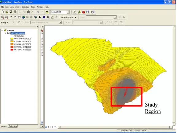
For the Charleston validation scenario, the refined data provided in URS (2001) (see

for an example hazard map) was adapted for MAEviz. A baseline MAEViz study of the Charleston area would typically use standard USGS attenuation functions for the Central and Eastern United States (CEUS), together with NEHRP soil amplification factors. However, the ground shaking hazard used by URS (2001) is heavily influenced by the work of Toro and Silva (2001), and in URS (2001), attenuation functions were selected and calibrated to reflect the geology of the region, and soil factors were also developed to reflect the local soil conditions in South Carolina, rather than applying NEHRP soil factors that were developed for the Western United States (Borcherdt, 1994; Dobry et al., 2000). In addition, the ground motion hazard maps produced by URS (2001) represent a weighted combination of both a point source and a finite fault model, and these maps were implemented with a 2 km x 2 km grid, rather than calculating hazard for centroids of census tracts.

Figure 1

Figure 2 [from Figure 4-27c of URS (2001)] illustrates the 7

(8)

source and associated rock PGAs for a median stress drop. From this map, the location of the center of the source can be estimated at 32º52’00”N, 80º16’40’’W. Ground shaking hazard maps are shown in Figures 4-27d through 4-30 of URS (2001), and have also been provided on the data DVDs supplied with HAZUS-MH (see Figure 3).

The supplied data on the HAZUS default data media was used to define ground shaking hazard in MAEViz for the validation study so as to minimize differences in hazard in the comparisons. The data on the HAZUS media was retained from the original report by URS (2001), and as such, it includes the joint effects of the combined finite fault model ground motions and the point source model ground motions, weighted by 0.8 and 0.2, respectively, together with refined parameters to account for site effects reflecting local geology.

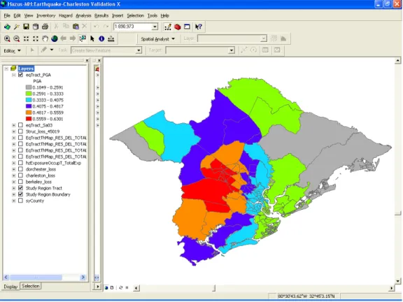
When using the hazard maps supplied from the study by URS (2001) in MAEViz, the data must be manipulated to prepare it for ingestion. HAZUS-MH is built as an extension to ArcGIS, and uses geodatabases containing polygon shapefiles to represent hazard. MAEViz uses only open source software, and uses an ASCII raster format for hazard maps. Since the general form of the data is fundamentally different between these representations (polygons in shapefiles versus gridded points in ASCII rasters), the reason for the use of the maps must be considered when transforming the data format. Since the MAEViz results will be compared with data obtained from a replicated HAZUS scenario, the primary requirement for the transformed data is that the hazard should be consistent at the centroids of census tracts. Census tracts can vary widely in size and shape throughout a study region. Therefore, a high resolution was chosen for the ASCII raster in an attempt to minimize any differences between HAZUS and MAEViz calculations. Figure 1 through Figure 6 show the progression of hazard map data manipulation. See Appendix A for further details on the steps taken to convert data from HAZUS to MAEviz.

(9)

Figure 1. Ground Motion Hazard from Charleston, SC Loss Assessment Study [from URS (2001)]

Figure 2. PGA on rock for Mw 7.3 event with median stress drop. [from URS (2001)]

(10)

Study Region

Figure 3. Surface PGA contours for Mw 7.3 (0.005 g intervals).

Figure 4. Surface PGA contours for Mw 7.3 at study region (0.005 g intervals). 10

(11)

Figure 5. Surface PGA resolved to census tracts.

Figure 6. Surface PGA raster imported to MAEViz. 11

(12)

Since the published results of URS (2001) consider the effects of ground failure, the scenario was replicated within the framework of the HAZUS methodology so that results may be obtained with liquefaction to verify that the results are consistent with published results of URS (2001), and without liquefaction for direct comparison with MAEViz results to facilitate equitable comparisons of loss estimation between MAEViz and the published losses in URS (2001). Liquefaction hazard in the HAZUS methodology is determined using liquefaction susceptibility ratings (from None to Very High), together with PGA. The liquefaction hazard is adjusted for duration through a modification factor in terms of moment magnitude and for the effect of soil saturation by a factor in terms of depth to ground water. Liquefaction susceptibility data was obtained from the HAZUS default data media, similarly to ground shaking hazard data, as shown in Figure 7. Liquefaction susceptibility correlates approximately to “Very High” for Factor of Safety < 0.6, and “None” for Factor of Safety > 1.8, as shown in Figure 8 [from Figure 5-12 of URS (2001)]. The depth to the ground water was taken as 2 feet in agreement with the value used by URS (2001). Additional details regarding calculation of liquefaction effects are provided in the Appendix.

URS (2001) also addressed landsliding. In their work, landsliding susceptibility was taken as Category I, which is the lowest susceptibility, for the entire Charleston region, based on the data provided in Figure 9 [from URS (2001)]. Landsliding hazard was thus neglected in this validation study, since the study region is almost entirely at the lowest available risk level for landsliding.

(13)

Figure 7. South Carolina liquefaction susceptibility

Figure 8. Liquefaction Safety Factors from Charleston, SC Loss Assessment Study [from URS (2001)]

(14)

Figure 9. Landslide Hazard from Charleston, SC Loss Assessment Study [from URS (2001)]

(15)

5INVENTORY DEFINITION

Inventory data used for the study by URS (2001) was collected in their research at the census block level and further adjusted with surveys and expert opinions of local professionals. The published results were obtained by using a final aggregation level of 2 km x 2 km grids. This data was then included in the default HAZUS inventory supplied with the installation media for HAZUS-MH MR2. In the validation study, the dispersion of inventory exposure for specific occupancy types throughout the study region was thus deemed to be consistent with URS (2001). In addition to the high geographic resolution used for the inventory, URS (2001) also revised the default occupancy-to-building type mapping schemes. URS (2001) defined four types of building “microzones”: Charleston’s historical district, urban (also includes Charleston outside the historical district), rural, and coastal. These areas are depicted in Figure 10 [from Figure 10-1 of URS (20010-1)].

The mapping schemes corresponding to the “microzones” were provided in Appendix F of URS (2001), and were originally applied to the refined 2 km x 2 km grid inventory. In this validation study, the mapping schemes are applied to the default inventory supplied with HAZUS (with the inventory data aggregated and supplied at the census track centroids). In an effort to generally conform to the original HAZUS input of URS (2001), accounting for the differences in the microzone mappings, each census tract was assigned a representative microzone and occupancy mapping scheme, based on the figures provided in URS (2001), as shown in . The mapping schemes are then used to assign building types with fragilities assumed to be appropriate in a Level I HAZUS study. In URS (2001), the fragility parameters were not modified from default HAZUS values.

Figure 11

(16)

Study Region

Figure 10. Building Inventory Microzonation from Charleston, SC Loss Assessment Study [from URS (2001)]

Figure 11. Approximate Building Zone Microzonation by Tract

(17)

Besides the adjustment for microzonation classification, exposure values were also calibrated to match the values given in Table 1 [from Table 10-4 of URS (2001)], which provides general occupancy exposures for each county.

Table 1. Charleston Region General Occupancy Exposures (in millions of dollars) [from URS (2001)]

County Residential Commercial Industrial Agriculture Religion Government Education Total

Charleston 11628 3189 218 5 132 72 334 15578

Furthermore, the data provided in Appendix F of URS (2001) indicates that the microzones contain the specific occupancies indicated in Table 2

Table 2. Specific Occupancies in Each Microzone .

Historic Urban Rural Coastal

RES1 X X X X RES2 X X X X RES3 X X X X RES4 X X X X RES5 X X X RES6 X X X COM1 X X X X COM2 X X X COM3 X X X X COM4 X X X COM5 X X X COM6 X X X COM7 X X X COM8 X X X X COM9 X X X X COM10 X X X X IND1 X X X IND2 X X X IND3 X X IND4 X X IND5 X X IND6 X X X AGR1 X X REL1 X X X GOV1 X X X GOV2 X X X EDU1 X X X EDU2 X X X

HAZUS currently uses a single occupancy mapping scheme for all tracts in the state of South Carolina. To adjust the default inventory so that the original scenario is more accurately represented, exposure values for specific occupancies which are not represented in Table 2 (e.g., IND3 through IND5 in a “Historic” tract) were purged, and the remaining exposures were scaled

(18)

to maintain a consistent exposure relative to the remaining value in the tracts with a total value for each general occupancy in each county matching the values provided in Table 1.

Finally, once the exposures for each specific occupancy in each tract had been adjusted, the HAZUS inventory data was converted from polygon- to point-type data to enable ingesting into MAEviz. HAZUS analyzes general building stock as polygon entities, but MAEViz uses point-wise general building stock input. To convert the polygon data to point data, a number of data tables were exported from HAZUS and used to generate “equivalent” lumped buildings. For each mapping scheme, HAZUS contains a data table indicating the percentage of buildings and exposure associated with a general structure type in a specific occupancy type. Hidden behind this table are additional tables that describe the distribution of specific structure types and code levels for each combination of specific occupancy and general structure type. Multiplying the appropriate values in the tables yields a set of direct conversion factors to partition total exposure for a given specific occupancy into a range of specific structure type and code level combinations. Thereafter, the inventory is treated identically between HAZUS and MAEViz for a Level I analysis. Additional details regarding microzone mapping scheme assignments and calibration of default HAZUS-MH MR2 inventory data are provided in Appendix A.

Table 3

Table 3. Charleston County Exposures by General Structure Type (in millions of dollars) [after Table 10-3 of URS (2001)] provides exposure values associated with general structure types. This data may be used to estimate the reliability of the conversion process from HAZUS default data to an inventory more closely resembling that used by URS (2001). Although the available data was transformed faithfully with respect to the published values, insufficient data was available to allow a fully accurate reconstruction of the inventory, which results in the inaccurate representation of various structure types. To account for the discrepancies shown in , contributions to aggregated final results were scaled individually for each general structure type in the Table. In addition, although the structure type distribution appears to deviate significantly from the data used in URS (2001), the impact on the aggregated final results in this case was found to be minor (approximately 1%).

User Wood Steel Concrete Precast RM URM MH Total

URS 6,890 1,176 1,622 1,084 548 3,804 454 15,578

MAEViz 7,851 1,730 1,297 231 960 3,185 321 15,577

%

difference 14% 47% -20% -79% 75% -16% -29% 0%

(19)

6REPLICATION OF HAZUS LOSS ESTIMATE

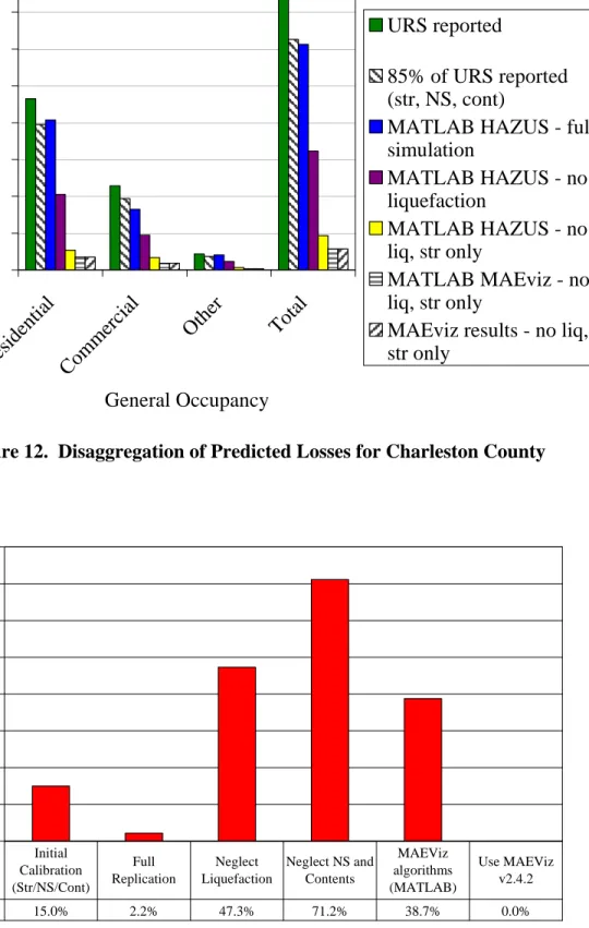
Calculations for damage and direct losses were computed using several methods to allow reasonable comparisons between results obtained from HAZUS and MAE Center methodologies. In the original study by URS (2001), the HAZUS methodology, including liquefaction, was applied to the study region to estimate potential losses. In order to compare the published results and the results obtained from MAEViz, loss calculations were first performed for direct economic loss by constructing a computational model in MATLAB consistent with the HAZUS methodology as described in the HAZUS Technical Manual (NIBS, 2003), as well as supplementary guidance from the appendix to a paper by Cao and Petersen (2006) detailing the HAZUS algorithms. The model used for this study addressed only structural, nonstructural, and contents losses. The other sources of direct economic loss considered in the HAZUS methodology, including inventory, relocation, capital related, wages, and rental income losses, were neglected in the computational model. A HAZUS-MH MR2 model was constructed using the hazard maps and a modified inventory database including the microzonations of URS (2001). In that model, the losses in the Charleston region for structural, nonstructural, and contents accounted for 85% of the total direct economic loss. Thus, results from the complete analysis within HAZUS were reduced by 15% so that comparisons with MAEviz could focus on structural, non-structural, and content losses.

The HAZUS model was executed for two cases for Charleston County: once each with and without liquefaction (“MATLAB HAZUS - full simulation” and “MATLAB HAZUS - no liquefaction”, respectively), because adequate data was not available to estimate damage including liquefaction within MAEviz. Results for structural losses only were then partitioned from the total losses for the case executed with no liquefaction (“MATLAB HAZUS – no liq, str only”) – it is this subset of the results that are used for the remaining comparisons. A model was then analyzed using a similar framework to the HAZUS computational model, except that MAE Center data and algorithms (e.g., Jeong and Elnashai, 2007; Bai et al., 2007) were substituted where appropriate (“MATLAB MAEViz – no liq, str only”). Finally, an analysis was performed using MAEViz (“MAEViz results - no liq, str only”). Details of the damage predictions (vulnerability model) and economic loss models used in the HAZUS and MAEviz methodologies are discussed and compared in more detail in the next section.

Damage predictions are made in HAZUS by applying the Capacity Spectrum Method (NIBS, 2003), whereas the fragilities in MAEViz were developed with the Parameterized Fragility Method (Jeong and Elnashai, 2007). Both methods rely on establishing limit state thresholds in terms of structural response of a first mode (SDOF) approximation of structures, either with displacements or with accelerations. For structural fragilities, peak relative displacement is the critical parameter. Although both methods rely on simplification of structural response so that only the first mode is considered, and both define fragility thresholds in terms of spectral

(20)

displacement, there are a number of fundamental differences between these two damage prediction methods.

The Capacity Spectrum Method is a nonlinear static analysis procedure that uses a number of simplifying assumptions to address issues such as duration of shaking and degradation of structural properties in order to approximate the peak displacement and acceleration experienced by a building during an earthquake. Parameters and algorithms used in the replicated HAZUS model, including the necessary parameters to apply the Capacity Spectrum Method for prediction of structural response, fragility parameters to correlate damage states with structural response, and damage factors to tie damage state prediction to direct losses in terms of dollars, were selected to be consistent with values used by URS (2001).

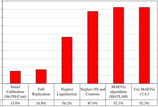
The Parameterized Fragility Method uses synthetically generated time history records in nonlinear time history analyses to obtain peak displacements for specified ground motion records that are deemed representative of ground motions in the region, and then correlates those peak displacements with ground shaking hazard parameters to define fragilities. In this study, peak displacements were correlated with peak ground acceleration, short period (0.3 second) 5% damped spectral acceleration, and moderate period (1.0 second) 5% damped spectral acceleration. Degradation effects are included directly in the constitutive model. Parameters and algorithms employed from Bai et al. (2007) are similar, but not identical, to the parameters and algorithms used by URS (2001) when tying damage to direct economic loss, with the primary observable difference occurring in the selection of mean damage factors used for the various damage states. The resulting total aggregated direct economic loss estimations for Charleston County are shown in Figure 12. Figure 13

Figure 13

and Figure 14 show the percentage change in the loss estimations from two perspectives: change of each calculation relative to the preceding value, and overall decrease of each calculation from the original total loss estimate provided in URS (2001) for Charleston County. In , a small difference (2.2%) is observed from the base case HAZUS results (URS, 2001) (which has 15% of the losses removed to account for losses other than structural, non-structural, and contents) as compared to the full simulation MATLAB HAZUS results. This is likely due to the assumptions made in transitioning the hazard and inventory data from the published report to the HAZUS implementation within MATLAB, or possibly due to discrepancies between the information provided in the HAZUS Technical Manual (NIBS, 2003) and the function of the algorithms within the program itself. Removing the effects of liquefaction changed the results more substantially, with a decrease of 47.3% from the estimated loss when liquefaction is included.

A decrease of 71.2%, relative to total replicated loss without including liquefaction, is observed when nonstructural and contents losses are neglected. This effect is consistent with the assumed distribution of building exposure in HAZUS among structural, nonstructural, and contents. Neglecting the COM10 (parking structures) and AGR1 (agriculatural facilities) occupancy types, structural value accounts for 4.6% to 19.4% of the total exposure (including

(21)

contents), with an average of 9.9%, and the structural losses account for 28.8% of the direct structural, nonstructural, and contents losses. The losses in structural value do not scale directly with the structural exposure because the fragility parameters (median and dispersion values defining lognormal cumulative density functions) are different for different types of damage (i.e., structural and drift-sensitive nonstructural, which use the same peak displacement to determine damage), and also because there are two damage indicators used to evaluate direct losses from ground shaking: spectral displacement for structural and drift-sensitive nonstructural, and an average spectral acceleration for acceleration-sensitive nonstructural and contents (Appendix B contains a full description of the algorithms used to replicate HAZUS calculations).

The differences discussed above highlight primary contributions to losses as predicted by HAZUS. Once the losses are isolated to structural damage with no liquefaction, the comparison to MAEviz results indicates that appreciable discrepancies still remain between loss estimates obtained from HAZUS and MAEViz, as seen in Figure 12, Figure 13, and Figure 14. Both the actual output from MAEViz (“MAEViz results – no liq, str only”) and the output from the MATLAB simulation of MAEViz (“MATLAB MAEViz – no liq, str only”) represent an average of three analysis runs, once each using fragilities calibrated to PGA, 0.3 second spectral acceleration, and 1.0 second spectral acceleration. A decrease of 38.7% in predicted structural loss is observed from the MATLAB HAZUS to the MATLAB MAEviz estimates. The “MATLAB MAEViz – no liq, str only”, and “MAEViz results - no liq, str only” differ in predicted losses by only 0.04%. Investigation of the source of the discrepancy between actual and simulated MAEViz results revealed that as part of the conversion process from shapefile hazard maps to rasters, some equivalent buildings which happened to be located on the border of a hazard step in the shapefile were assigned a hazard from the raster which was 0.05 g higher or lower than the value assigned by intersecting the inventory location with the shapefile. The results indicate that the algorithmic implementation for direct structural losses in MAEViz is consistent with the guidance provided by the published algorithms (Steelman et al., 2006; Jeong and Elnashai, 2007; Bai et al., 2007). The differences between the “MATLAB HAZUS – no liq, str only” and the “MATLAB MAEViz – no liq, str only” and “MAEViz results – no liq, str only” cases are therefore determined to be systematically embedded in the respective methodologies, and are discussed in detail in the following sections.

(22)

$-$1.0 $2.0 $3.0 $4.0 $5.0 $6.0 $7.0 $8.0 Res iden tial Commerc ial Oth er Total General Occupancy P red icted Lo ss ( B illio n s o f D o llar s) URS reported 85% of URS reported (str, NS, cont)

MATLAB HAZUS - full simulation MATLAB HAZUS - no liquefaction MATLAB HAZUS - no liq, str only MATLAB MAEviz - no liq, str only

MAEviz results - no liq, str only

Figure 12. Disaggregation of Predicted Losses for Charleston County

0.0% 10.0% 20.0% 30.0% 40.0% 50.0% 60.0% 70.0% 80.0% P erc ent Re du ct io n R ela tiv e t o P re ced in g S tag e 15.0% 2.2% 47.3% 71.2% 38.7% 0.0% Initial Calibration (Str/NS/Cont) Full Replication Neglect Liquefaction Neglect NS and Contents MAEViz algorithms (MATLAB) Use MAEViz v2.4.2

Figure 13. Percent Reduction of Losses at Each Stage of Loss Disaggregation Relative to Previous Stage

(23)

0.0% 10.0% 20.0% 30.0% 40.0% 50.0% 60.0% 70.0% 80.0% 90.0% 100.0%

Percent Reduction Relative to T

o ta l Reported Los s 15.0% 16.8% 56.2% 87.4% 92.3% 92.3% Initial Calibration (Str/NS/Cont) Full Replication Neglect Liquefaction Neglect NS and Contents MAEViz algorithms (MATLAB) Use MAEViz v2.4.2

Figure 14. Percent Reduction of Losses at Each Stage of Loss Disaggregation Relative to Total Reported Loss Estimate

(24)

7COMPARISON OF HAZUS AND MAEViz DIRECT ECONOMIC LOSS

There are two fundamental differences between the algorithms and data used in the “MATLAB HAZUS – no liq, str only” and the “MATLAB MAEViz – no liq, str only” cases: the vulnerability functions and loss functions establishing correlation between physical damage and economic loss. The lesser of the two influences is the difference between loss functions. In both cases, an expected loss is calculated by applying the equation

)

* (1)

[

]

(

)

1 * i n i DF i E Loss Exposure P DS DS μ = =

∑

= Where

Exposure = dollar value exposure of inventory entity

n = number of discrete damage states (5 in HAZUS, 4 in MAEViz) P(*) = probability of occurrence of (*)

DS = damage state

i

DF

μ = mean damage factor correlating to damage state i

In accordance with Bai et al. (2007), damage states are considered to be approximately equivalent on a one-to-one basis between HAZUS and MAE Center algorithms. The HAZUS-MH structural damage factors [

i

DF

μ in Equation (1)] may be determined from the values provided in Table 15.2 of the HAZUS-MH MR2 Technical Manual (NIBS, 2003). A comparison of the damage states and structural damage factors for the HAZUS and MAE Center methodologies (after Bai et al., 2007) is provided in Table 4. There are only minor differences in the two frameworks for damage-to-loss correlation. Relative to HAZUS, the MAE Center Insignificant damage state may be viewed as a combination of the HAZUS damage states None and Slight. It should also be noted that the MAE Center framework is inherently a probabilistic model, and focuses on providing estimates of uncertainty together with expected values. For this reason, the MAE Center minimum damage factor is greater than 0, and the maximum damage factor is less than 1.

(25)

Table 4. Comparison of HAZUS and MAE Center Damage States and Factors

HAZUS MAE Center

Damage State Damage Factor Damage State Damage Factor

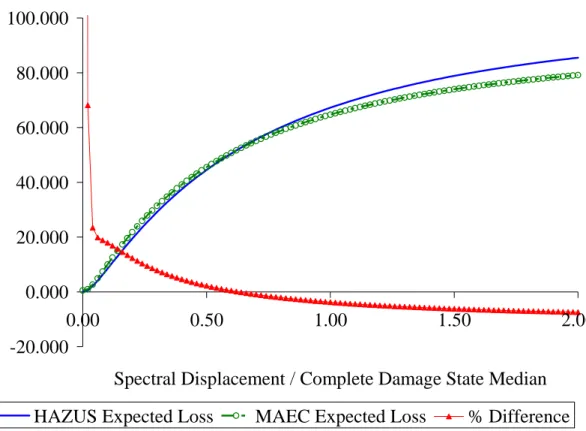
None 0 Slight 0.02 Insignificant 0.005 Moderate 0.10 Moderate 0.155 Extensive 0.50 Heavy 0.55 Complete 1.00 Complete 0.90 To examine the effects of the differences in damage factors, plots were generated by

considering damage for a wide range of hazard magnitudes, represented by varying peak spectral displacement, which is the key input parameter for the structural damage vulnerability functions. In Figure 15, calculations have been performed assuming a range of spectral displacement normalized by the median spectral displacement at the threshold of Complete Damage for a Low-Rise W1 Light Wood Frame Structure. For this plot, differences in vulnerability between HAZUS and the Jeong and Elnashai (2007) were neglected by calculating damage state probabilities in accordance with HAZUS fragilities, then applying the HAZUS and Bai et al. (2007) damage factors to identical sets of discrete damage state probabilities. The HAZUS and MAE Center (MAEC) curves indicate expected structural loss in percent as a function of normalized spectral displacement.

(26)

-20.000 0.000 20.000 40.000 60.000 80.000 100.000 0.00 0.50 1.00 1.50 2.00

Spectral Displacement / Complete Damage State Median

% Lo

ss or % D

ifferen

ce

HAZUS Expected Loss MAEC Expected Loss % Difference

Figure 15. Comparison of Loss Ratios for a Low-Rise W1 Light Wood Frame Structure Figure 15 shows that the net effect of the discrepancies in damage factors are often small relative to the differences shown in Figure 12

Figure 12 Figure 12

. Looking at the curve labeled “% Difference” in the figure, the largest discrepancies by percentage occur for very light damage, when dividing by a number much less than 1 can result in a significant amplification in the calculation of percent difference, although the absolute value of the difference in structural damage factors tends to 0.5%. Analyses performed using HAZUS damage factors in place of MAE Center damage factors, but retaining MAE Center damage estimation algorithms and parameters, resulted in a decrease of approximately 3.7% in the loss estimate from the value shown in . The primary discrepancy between the HAZUS and MAEviz results of must therefore originate in the vulnerability functions.

(27)

8COMPARISON OF HAZUS AND MAEViz DAMAGE PREDICTION 8.1Development of Ground Motion Records

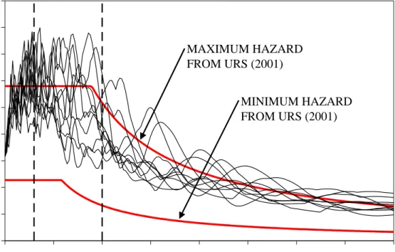
In order to maintain consistent hazard spectra for the loss assessment and ground motions used in the development of parameterized fragilities, and thereby allow a more reliable comparison with the values produced by URS (2001), ten synthetic ground motion records were generated using SIMQKE-I (Vanmarcke et al., 1990) to match more closely with the maximum hazard acceleration response spectra used by URS (2001). Plots of the acceleration response spectra for individual records and a smoothed average acceleration response spectrum are shown in Figure 16 and Figure 17 along with the acceleration response spectra corresponding to the minimum and maximum spectra used in URS (2001) for the study region.

0 0.2 0.4 0.6 0.8 1 1.2 1.4 1.6 1.8 0 0.5 1 1.5 2 2.5 3 3.5 4 Period, T (sec) Spec tr al Ac ce le ra ti on, Sa (g ) MAXIMUM HAZARD FROM URS (2001) MINIMUM HAZARD FROM URS (2001)

Figure 16. SIMQKE-I ground motion record spectra

(28)

0 0.2 0.4 0.6 0.8 1 1.2 1.4 1.6 1.8 0 0.5 1 1.5 2 2.5 3 3.5 4 Period, T (sec) Spec tr al Ac ce le ra ti on, Sa (g ) MAXIMUM HAZARD FROM URS (2001) MINIMUM HAZARD FROM URS (2001) AVERAGE HAZARD

FROM SIMQKE-I RECORDS

Figure 17. Smoothed Average SIMQKE-I ground motion record spectrum

Using the SIMQKE-I records to develop parameterized fragilities for the Charleston region, loss estimates for Charleston County were approximated at $570,580,000 due to direct loss of structural value when using a PGA hazard index obtained from shapefile intersections (using identical hazard values to those used in the MATLAB HAZUS model, corresponding to “MATLAB MAEViz – no liq, str only” in Figure 12

Figure 12

Figure 12 ), or $570,810,000 when using raster hazard maps (corresponding to “MAEViz results – no liq, str only” in ). As indicated previously, the observed discrepancy between loss estimates using the MAEViz methodology with shapefile versus raster hazard data is about 0.04%. The prediction of direct loss of structural value obtained from application of the HAZUS Capacity Spectrum Method, however, is about $931,430,000 (corresponding to “MATLAB HAZUS – no liq, str only” in ). 8.2Inclusion of Degradation in Parameterized Fragility Model

To investigate the source of the remaining discrepancy, the next section describes a comparison of the nonlinear static analysis procedure for estimating damage in HAZUS versus the nonlinear dynamic analysis methodologies for estimating damage in MAEviz. The most significant difference between the two methods was found in the treatment of degradation, which in this context is meant to refer to an aggregate effect of losses in strength and stiffness and also how damage to the structure is manifested in the force-displacement relationship of the

(29)

representative SDOF’s used for analysis. To explore these differences in depth, hysteretic models were developed to represent commonly expected behavior (e.g., strength degradation) based on the brief description of expected hysteretic behavior provided in the HAZUS Technical Manual (NIBS, 2003).

The parameterized fragilities were originally derived by using a bilinear kinematic model for an SDOF with a uniaxial load-deformation response (Jeong and Elnashai, 2007). Since the capacity curves for HAZUS buildings exhibit perfectly plastic behavior, the bilinear model used for the parameterized fragilities was initially elastic-perfectly-plastic. This model assumes that a structure will exhibit full hysteresis loops when subjected to cyclic excursions into the plastic range during a time history analysis. The Capacity Spectrum Method does not explicitly characterize the shape of the hysteretic curves under cyclic demand, but does include a κ factor to account for degradation in a general sense (see Appendix B). Several models were therefore implemented in the parameterized fragility analysis engine to account for degradation in a manner deemed representative of the more generalized approach used within the Capacity Spectrum Method in HAZUS. Hysteretic rule sets were applied to specific structure types according to expected dominant mechanisms (see Chen et al., 2008; Ellingwood et al., 2008; Folz and Filiatrault, 2004; Foutch and Yun, 2002; Franklin et al., 2001; Hidalgo et al., 2002; Hidalgo et al., 2002; Ibarra et al., 2005; NIBS, 2003, Remennikov and Walpole, 1997; Sivaselvan and Reinhorn, 2000; Tremblay, 2002; Tremblay et al., 2003; Voon, 2007; Yi et al., 2006; Yi et al., 2006). The applied rule sets for each structure type are detailed in Table 5.

(30)

Table 5. Hysteretic Model Assignments by Structure Type

HAZUS Label HAZUS Description Hysteretic Model Reference

W1 Light Wood Frame Pinching

W2 Commercial and Industrial Wood Frame Pinching

S1L Low-Rise Steel Moment Frame Bilinear

S1M Mid-Rise Steel Moment Frame Bilinear

S1H High-Rise Steel Moment Frame Bilinear

S2L Low-Rise Steel Braced Frame Pinching

S2M Mid-Rise Steel Braced Frame Pinching

S2H High-Rise Steel Braced Frame Pinching

S3 Steel Light Frame Bilinear *** See S1 (NIBS, 2003) ***

S4L Low-Rise Steel Frame w/ CIP Concrete Shear Walls Pinching

S4M Mid-Rise Steel Frame w/ CIP Concrete Shear Walls Pinching

S4H High-Rise Steel Frame w/ CIP Concrete Shear Walls Pinching

S5L Low-Rise Steel Frame w/ Unreinforced Masonry Infill Walls Flag-Shaped S5M Mid-Rise Steel Frame w/ Unreinforced Masonry Infill Walls Flag-Shaped S5H High-Rise Steel Frame w/ Unreinforced Masonry Infill Walls Flag-Shaped

C1L Low-Rise Concrete Moment Frame Pinching

C1M Mid-Rise Concrete Moment Frame Pinching

C1H High-Rise Concrete Moment Frame Pinching

C2L Low-Rise Concrete Frame w/ Shear Walls Pinching

C2M Mid-Rise Concrete Frame w/ Shear Walls Pinching

C2H High-Rise Concrete Frame w/ Shear Walls Pinching

C3L Low-Rise Concrete Frame w/ Unreinforced Masonry Infill Walls Flag-Shaped C3M Mid-Rise Concrete Frame w/ Unreinforced Masonry Infill Walls Flag-Shaped C3H High-Rise Concrete Frame w/ Unreinforced Masonry Infill Walls Flag-Shaped

PC1 Concrete Tilt-Up Pinching *** See C2 (NIBS, 2003) ***

PC2L Low-Rise Precast Concrete Frame Pinching

PC2M Mid-Rise Precast Concrete Frame Pinching

PC2H High-Rise Precast Concrete Frame Pinching

RM1L Low-Rise Reinforced Masonry Bearing Walls with Wood or Metal Deck Diaphragms Pinching RM1M Mid-Rise Reinforced Masonry Bearing Walls with Wood or Metal Deck Diaphragms Pinching RM2L Low-Rise Reinforced Masonry Bearing Walls with Precast Concrete Diaphragms Pinching RM2M Mid-Rise Reinforced Masonry Bearing Walls with Precast Concrete Diaphragms Pinching RM2H High-Rise Reinforced Masonry Bearing Walls with Precast Concrete Diaphragms Pinching

URML Low-Rise Unreinforced Masonry Bearing Walls Flag-Shaped

URMM Mid-Rise Unreinforced Masonry Bearing Walls Flag-Shaped

MH Mobile Homes Pinching *** See W (NIBS, 2003) ***

Ellingwood et al., 2008; Folz and Filiatrault, 2004; Ibarra et al., 2005 Foutch and Yun, 2002; Ibarra et al., 2005; Sivaselvan and Reinhorn, 2000 Reminnikov and Walpole, 1997; Tremblay, 2002; Tremblay et al., 2003

*** See C2 (NIBS, 2003) ***

Voon, 2007

Chen et al., 2008; Franklin et al., 2001; Yi et al., 2006; Yi et al., 2006 *** See URM (NIBS, 2003) ***

Hidalgo et al., 2002; Ibarra et al., 2005

Hidalgo et al., 2002; Hidalgo et al., 2002

(31)

As indicated in Table 5, the most frequently assigned model was a pinching model. The fundamental hysteretic rules of the model follow the pinching model described in Ibarra et al. (2005), with some modifications. In the Ibarra et al. (2005) pinching model, once an excursion has been completed, the force-displacement curve in the opposite direction is adjusted, except for the unloading stiffness adjustment. Also, multiple distinct degradation mechanisms are adjusted for individually. For the pinching model implemented in the parameterized fragilities, in an attempt to match as closely as possible to the HAZUS formulation, the force-displacement relation is updated simultaneously in both directions at the instant load reversal takes place, and only when a new peak displacement has been reached. The updated force-displacement relation assumes that the target peak displacement is always the same in both directions, unlike the Ibarra et al. (2005) model which tracks the target displacement in positive and negative directions separately. The decision to create this rule was based on the description of the hysteretic energy term in the HAZUS Technical Manual (NIBS, 2003), where the performance point is defined by the peak displacement response and the acceleration at peak displacement response, and associated hysteretic energy obtained from the Capacity Spectrum Method is a function of the performance point location as well as “the area enclosed by the hysteresis loop, as defined by a symmetrical push-pull of the building capacity curve up to peak positive and negative displacements.”

In the equation shown in the HAZUS Technical Manual (NIBS, 2003) to calculate the hysteretic energy term, the κ factor is multiplied by the area of the full hysteresis loop, which is assumed to define the enclosed area of the pinched hysteresis loop. Therefore, if the κ factor is given, along with a peak inelastic displacement and acceleration, two assumptions are required in order to uniquely define the degraded constitutive relation: the slope of the unloading stiffness and the path of possible break points. In this case, the unloading stiffness was assumed to be constant, similarly to the plywood examples provided in Ibarra et al. (2005), and all possible break points are assumed to lie on a straight line from the intersection of the unloading path with the horizontal axis to the yield point in loading with full hysteresis. Figure 18 and are provided to compare the two force-displacement relations used in the development of parameterized fragilities before and after implementing the pinching model, respectively. The pinching model shown conforms to pinching expected of a W1 Pre-Code building during a “Moderate” duration earthquake (moment magnitude between 5.5 and 7.5), with a κ factor of 0.30.

(32)

-1.5 -1 -0.5 0 0.5 1 1.5 -6 -5 -4 -3 -2 -1 0 1 2 3 4 5 6

Displacement Normalized by Yield

Force Norm

alized by Yield

A

B

C

D

J

I

H

G

F

E

Figure 18. Original bilinear response implemented in parameterized fragilities

-1.5 -1 -0.5 0 0.5 1 1.5 -6 -5 -4 -3 -2 -1 0 1 2 3 4 5 6

Displacement Normalized by Yield

Force Norm

alized by Yield

A

B

C

D

J

I

H

G

F

E

O

N

M

L

K

Figure 19. Pinching response implemented in revised parameterized fragilities 32

(33)

The slopes of the lines from points B to C, E to F, I to J, and L to M are all equal, and unchanged from the initial elastic stiffness of the system. Points D and G, and K and N were calculated so that the area included in the hysteresis loop would be 30% of the area of a full hysteresis loop, in accordance with the specified κ factor. Also, the definition of response characteristics when the response falls within the pinched envelope must be defined. There are two sub-classes which were used for this study: κ less than 0.5, and κ greater than or equal to 0.5. In actuality, the κ factor will be less than or equal to 0.4 for all structures in the study region based on the values in the HAZUS Technical Manual (NIBS, 2003), but rules were also developed for larger κ factors such that a smooth transition could be defined up to a value of 1 (full hysteresis) when investigating the effects of varying the κ factor.

Where κ is less than 0.5, a critical displacement is defined by extrapolating the loading curve from the break point to the peak displacement back to the horizontal axis. If the dynamic response leaves the envelope and intersects the horizontal axis at a greater displacement (in the sense of a positive loading direction) than this critical displacement value, then the loading proceeds directly from the horizontal axis to the peak displacement, bypassing the pinched break point. If the intersection is less than or equal to the critical displacement, the loading proceeds first to the break point, then to the peak point. This is similar to the behavior in Ibarra et al. (2005), however, according to the rules given in that paper, if the intersection displacement is infinitesimally smaller than the break point displacement, there would be a nearly vertical loading branch to the break point before continuing from the break point to the peak displacement. The definition of the critical displacement for this study precludes the evolution of an infinitely stiff loading branch, and ensures that all loading branches will have stiffness values between elastic stiffness at a maximum, and pre-break point stiffness at a minimum, where both extremes exist solely on the pinched envelope. Example applications of the rules for

κ less than 0.5 are shown in Figure 20.

(34)

-1.5 -1 -0.5 0 0.5 1 1.5 -6 -5 -4 -3 -2 -1 0 1 2 3 4 5 6

Displacement Normalized by Yield

Force Norm

alized by Yield

A

B H

M.2

L.1

G

C

D

J.1

I

F

E

K.1

L.2

K.2

J.2

Figure 20. Pinching behavior within envelope for κ = 0.3

Where κ is greater than or equal to 0.5, a critical displacement is also defined. However, the displacement is based on following an elastic loading branch back from the break point to the horizontal axis. It was necessary to redefine this particular rule for large values of the κ factor, since the loading branches pre- and post-break point are collinear for κ equal to 0.5, and the critical displacement defined by the previous rule would lie outside of the pinched envelope for larger values of the κ factor. For large values of κ, if the intersection point is larger than the critical displacement, the loading follows an elastic loading branch until it intersects the post-break point envelope, at which point it continues to follow the envelope. If the intersection point is less than the critical displacement, then the rule is the same as for small κ factors, with loading proceeding first to the break point, then to the peak displacement. Example applications of the rules for κ greater than or equal to 0.5 are shown in Figure 21.

(35)

-1.5 -1 -0.5 0 0.5 1 1.5 -6 -5 -4 -3 -2 -1 0 1 2 3 4 5 6

Displacement Normalized by Yield

Force Norm

alized by Yield

A

B H

C

D

J

I

G

F

E

M.2

L.1

K.1

K.2

L.2

M.1

N

Figure 21. Pinching behavior within envelope for κ = 0.8

Figure 21

Two alternate load paths are shown in each of the figures to illustrate these rules. In Figure 20, the maximum displacement occurred at point B, and the pinched curves are defined at that step in the load history for each of the alternative cases. For illustrative purposes, loading proceeds up to point 9 identically for each of the alternative cases, so that the envelope of pinched response is fully developed in the load history. In the first case, load reversal occurs at J.1, followed by elastic unloading to K.1. The displacement at K.1 is greater than the critical displacement, where the dashed line extending back from point G intersects the horizontal axis, so the loading proceeds directly to the peak displacement at L.1. If load reversal occurs later, at J.2, then the elastic unloading to K.2 results in an intersection point less than the critical displacement, so loading proceeds first to the break point at L.2, then to the peak displacement at M.2.

For cases with large values for the κ factor, as in , the critical displacement follows the alternate definition as shown. In this case, M.1 lies on the post-break point loading path, rather than falling directly at the peak displacement. An effective break point is defined in this case by shifting the true break point along the post-break point loading curve envelope, rather than ignoring the break point and the loading path from the break point to peak point entirely. If the value of the κ factor is exactly equal to 1, then this set of hysteretic rules results in the original bilinear elastic-perfectly-plastic model used when developing the parameterized fragilities (Jeong and Elnashai, 2007).

(36)

Hysteretic formulations were also implemented to represent degrading bilinear behavior, as would be expected for steel moment frames, and a flag-shaped hysteresis, similar to a slip-model, which would be expected when seismic response is dominated by rocking or toe-crushing mechanisms in unreinforced masonry. For the degrading bilinear hysteresis, when a load reversal occurs at a new peak displacement in the plastic range, the elastic unloading and reloading stiffness is reevaluated such that the enclosed space of a hysteretic loop will equal the area of a full hysteretic loop scaled by the κ factor. An example of the degrading bilinear hysteretic rules is shown in Figure 22.

-1.5 -1 -0.5 0 0.5 1 1.5 -6 -5 -4 -3 -2 -1 0 1 2 3 4 5 6

Displacement Normalized by Yield

Force Norm

alized by Yield

F,J

A E B I

G D C

H

Figure 22. Degrading bilinear behavior for κ = 0.3

For the flag-shaped hysteretic rules governing unreinforced masonry exhibiting flexural mechanisms, elastic loading and unloading stiffness is held constant. When in the plastic range, unloading from the plastic loading branch proceeds first by an elastic unloading branch from the load reversal point, followed by a plastic unloading branch parallel to the plastic loading branch. The plastic unloading branch extends back to the initial elastic loading branch, where unloading proceeds back through the origin to the diametrically opposing quadrant. An example of the hysteretic rules for unreinforced masonry governed by flexural mechanisms is shown in Figure 23.

(37)

-1.5 -1 -0.5 0 0.5 1 1.5 -6 -5 -4 -3 -2 -1 0 1 2 3 4 5 6

Displacement Normalized by Yield

Force Norm

alized by Yield

A,I,Q

B

J

C

D,L

H,P

G

F

E,M

K

O

N

Figure 23. Degrading unreinforced masonry behavior for κ = 0.3

Loss calculations were performed using the Parameterized Fragility Method and the Capacity Spectrum Method, both with and without the inclusion of degradation. The loss estimate obtained from the Parameterized Fragility Method using constitutive models that neglect degradation shows a decrease in losses of approximately 13.1% overall when compared to the loss estimate including degradation. When the losses were recalculated using the Capacity Spectrum Method for the replicated HAZUS analysis methodology, but forcing the degradation factor to 1 for all structure types and code levels to investigate the effect of degradation on the losses calculated by the Capacity Spectrum Method approach, losses were observed to decrease by 68.1%. Calculated values of direct losses in terms of structural replacement cost with and without considering degradation and by Capacity Spectrum Method and the Parameterized Fragility Method are shown in Figure 24.

(38)

PFM CSM $0 $100,000,000 $200,000,000 $300,000,000 $400,000,000 $500,000,000 $600,000,000 $700,000,000 $800,000,000 $900,000,000 $1,000,000,000 Expected Los s ($) Fragility Method Degradation Included Degradation Excluded PFM $570,600,000 $496,000,000 CSM $931,400,000 $296,700,000

Degradation Included Degradation Excluded

Figure 24. Structural Loss Estimate Variation with respect to Fragility Method and Consideration of Degradation Effects

(39)

8.3Effect on Response of Variations in Selected Parameters

The effect of varying the κ factor and ground motion level was investigated by calculating predicted displacements using both the parameterized fragility nonlinear time history engine with the hysteretic degradation rules described above, as well as the HAZUS Capacity Spectrum Method, for a Pre-Code URML and a Low-Code W2 SDOF. When the URML structure was assigned a κ factor greater than 0.5, the flag-shaped hysteresis rules would predict a permanent displacement (tilt) of the URM shear walls. To attempt to capture more realistic results for large values of κ, the constitutive model was shifted to a bilinear model for κ factors greater than 0.5 for the URML structure type. This constitutive model reflects a bed-joint sliding mechanism rather than a rocking mechanism, which is more appropriate as the hysteresis approaches full loops without degradation. The motivation for the selection of these structure types originates from the investigation of the effect of degradation, where the URML structure type showed the least influence from degradation on average (2.4%), and the W2 structure type showed the greatest influence on average (33.9%).

Analyses were carried out by scaling records from 0g to 1g PGA in increments of 0.05g, and also assuming κ factors ranging from 0 to 1 in increments of 0.05. Each plotted point for the displacement predictions represents the average of the results of the ten SIMQKE-I records after passing each record through the nonlinear time history analysis engine to obtain the Parameterized Fragility Method (PFM) prediction of displacement demand, and using a smooth spectrum based on 0.3 second and 1 second spectral accelerations for each record to obtain the Capacity Spectrum Method (CSM) predicted displacement demand. The results of these analyses are plotted in Figure 25 through Figure 30. The results shown represent the average of the outputs of the ten SIMQKE-I generated records. Actual predictions are plotted for each structure type and analysis method, followed by a comparison of the results of the two methods. Comparisons are presented as ratios of predicted displacements obtained from the CSM to those obtained from the PFM. Both damage prediction methods rely on two components: the prediction of displacement demand for the structure imposed by the hazard, and limit state thresholds defined in terms of displacement to distinguish between damage states. Damage predictions based on both methods include identical limit state thresholds for damage states, so differences in predicted damage can be traced directly to predictions of displacements.

(40)

Figure 25. Average displacement from PFM analysis of a Pre-Code URML SDOF

Figure 26. Average displacement from CSM analysis of a Pre-Code URML SDOF 40

(41)

Figure 27. Average displacement from PFM analysis of a Low-Code W2 SDOF

Figure 28. Average displacement from CSM analysis of a Low-Code W2 SDOF 41

(42)

Figure 29. Comparison of analysis outputs for a Pre-Code URML SDOF

Figure 30. Comparison of analysis outputs for a Low-Code W2 SDOF 42

(43)

While the results shown in these figures are specific to the structure types shown, a general pattern is clearly observable. The Capacity Spectrum Method frequently predicts larger displacements than does the Parameterized Fragility Method’s nonlinear time history engine. This trend increases with decreasing degradation factor (i.e., with increasingly degraded response). For this scenario, approximately 97% of the inventory exposure is coupled with a degradation factor of 0.2 or 0.3.

There is generally not an exact correlation from differences in predicted displacement response to discrepancies in loss prediction when evaluating how observed discrepancies in direct loss prediction arise from differences in predicted displacement response. When displacement response is amplified, the effect on loss will depend on where the response lies on the lognormal CDF of the fragility function. For very small or very large displacements, a change in the displacement value may not be significant, as opposed to when predictions lie near the median. Additionally, it is necessary to consider how the fragility curves are drawn relative to each other, as damage state probabilities are taken as the difference of adjacent limit state exceedence probabilities. Values of damage factors can also play a role, especially for higher damage states. For example, increasing the probability of the Moderate damage state, with a damage factor of 15.5%, will not affect results as significantly as an identical increase in the probability of the Complete damage state, with a damage factor of 90%. Examples of the aggregate of these effects are shown in Figure 31 through Figure 33.

0.0

50.0

100.0

150.0

200.0

250.0

300.0

350.0

0.15

0.35

0.55

PGA (g)

Pred

icted D

isp

lacement (mm)

W2 PC CSM

W2 PC NLTH

W2 LC CSM

W2 LC NLTH

URML PC CSM

URML PC NLTH

URML LC CSM

URML LC NLTH

Figure 31. Variation in Predicted Displacement with respect to Ground Shaking 43

(44)

0.0000

0.1000

0.2000

0.3000

0.4000

0.5000

0.6000

0.7000

0.8000

0.9000

0.15

0.35

0.55

PGA (g)

Predicted

Damage Factor

W2 PC CSM

W2 PC NLTH

W2 LC CSM

W2 LC NLTH

URML PC CSM

URML PC NLTH

URML LC CSM

URML LC NLTH

Figure 32. Variation in Predicted Damage Factor with respect to Ground Shaking

0.00

1.00

2.00

3.00

4.00

5.00

6.00

7.00

8.00

9.00

10.00

0.15

0.35

0.55

PGA (g)

Pred

iction

R

a

tio (CS

M / PFM)

W2 PC

displacement

W2 LC

displacement

URML PC

displacement

URML LC

displacement

W2 PC Loss

W2 LC Loss

URML PC Loss

URML LC Loss

Figure 33. Variation in Prediction Ratios with respect to Ground Shaking

(45)

In Figure 31

Figure 31

, the difference in predicted displacements for URML and W2 structure types is shown for a range of PGAs from 0.19g to 0.61g, which is the range of PGA intensities to which the structures are subjected. The URML PC (Pre-Code) and W2 LC (Low-Code) curves are identical to sections taken through Figure 25 to Figure 28 at appropriate values of κ. In Figure 32

Figure 32

, the predicted displacements from have been converted to mean damage factors by evaluating probabilities of limit state exceedence, taking differences of adjacent exceedence probabilities to calculate damage state probabilities, and pairing discrete damage state probabilities with damage factors (using factors appropriate for HAZUS with the CSM results, and using MAE Center damage factors with PFM results). The shapes of the curves plotted in

do not match with those plotted in .

In Figure 33, the ratios of CSM to PFM engine results for both displacements and damage factors are plotted for the considered structure types and code levels. The ratios of predicted displacements increase or remain level along the full range of ground shaking demands, but the ratios of the losses are observed to decrease for some of the higher demand levels, most notably for Low-Code W2 structures. Furthermore, for the URML structures, the ratios of losses were generally less than the ratios of the displacements, while for the W2 structures, the opposite pattern is observed, with the ratios of the losses generally higher than the ratios of the displacements. These outcomes reveal the complex interplay of response and limit state parameters, even for the greatly simplified SDOF representation of structures used commonly in regional seismic loss assessments, with regard to not only predicted nonlinear displacement demands for structures over a range of ground motion intensities, but also to the resiliency of those structures to resist the imposed demands.

(46)

9CONCLUSION

A loss assessment originally performed using HAZUS-99 for the State of South Carolina was replicated and used to validate the capabilities of MAEViz to perform a similar study. MAEViz was found to synthesize the various aspects of a loss assessment study well. As with any software, the validity of the results will depend on the veracity of the assumptions used in developing the algorithms as well as the reliability of the original input datasets. MAEViz cannot directly replicate the results of the South Carolina study because it does not include an algorithm to perform the Capacity Spectrum Method (CSM) used by HAZUS. However, the results obtained from the CSM were scrutinized in this study to compare the predicted structural response with predictions obtained from the use of time history analyses.

Nonlinear time history analyses were performed using constitutive modeling of uniaxial SDOF oscillators in the Parameterized Fragility Method (PFM) to reflect the parameters and algorithms incorporated in the HAZUS CSM. The CSM results were found to provide markedly different results from the PFM, with or without the inclusion of degradation effects in the structural response. For the ground motion records and the structural characteristics of the inventory considered in this study, the CSM was found to be more sensitive than the PFM to the effects of degradation, and CSM results bracketed the values obtained using the PFM to evaluate damage and direct economic loss.

(47)

10REFERENCES

Abrams, D. P. and Shinozuka, M. (eds.) (1997). “Loss Assessment of Memphis Buildings,” Technical Report No. NCEER-97-0018, National Center for Earthquake Engineering Research, State University of New York at Buffalo, Buffalo, New York.

Bai, J. W., Hueste, M., and Gardoni, P. (2007). “Probabilistic Assessment of Structural Damage due to Earthquakes for Buildings in Mid-America,” Journal of Structural Engineering, ASCE, submitted for publication.

Ballantyne, D., Bartoletti, S., Chang, S., Graff, B., MacRae, G., Meszaros, J., Pearce, I., Pierepiekarz, M., Preuss, J., Stewart, M., Swanson, D., and Weaver, C. (2005). Scenario for a Magnitude 6.7 Earthquake on the Seattle Fault, Earthquake Engineering Research Institute, Oakland, California.

Borcherdt, R. D. (1994). “Estimates of Site-Dependent Response Spectra for Design (Methodology and Justification),” Earthquake Spectra,Vol. 10, pp. 617-653.

Cao, T. and Petersen, M. D. (2006). “Uncertainty of Earthquake Losses due to Model Uncertainty of Input Ground Motions in the Loss Angeles Area,” Bulletin of the Seismological Society of America, Vol. 96, No. 2, pp. 365-376.

Central United States Earthquake Consortium (CUSEC) (1985). “An Assessment of Damage and Casualties for Six Cities in the Central United States Resulting from Earthquakes in the New Madrid Seismic Zone,” Internal Report, Federal Emergency Management Agency, Washington, DC.

Central