Oil price volatility and stock returns in the G7 economies

(1)

Facultad de Ciencias Económicas y Empresariales

Working Paper nº 01/16

Oil price volatility and stock returns

in the G7 economies

Elena Maria Diaz

University of Navarra

Juan Carlos Molero

University of Navarra

Fernando Perez de Gracia

(2)

Oil price volatility and stock returns in the G7 economies

Elena Maria Diaz, Juan Carlos Molero and Fernando Perez de Gracia January 2016

ABSTRACT

This study examines the relationship between oil price volatility and stock returns in the G7 economies (Canada, France, Germany, Italy, Japan, the UK and the US) using monthly data for the period 1970 to 2014. In order to measure oil volatility we consider alternative specifications for oil prices (world, nominal and real prices). We estimate a vector autoregressive model with the following variables: interest rates, economic activity, stock returns and oil price volatility taking into account the structural break in the year 1986. We find a negative response of G7 stock markets to an increase in oil price volatility. Results also indicate that world oil price volatility is generally more significant for stock markets than the national oil price volatility.

Elena Maria Diaz University of Navarra Juan Carlos Molero University of Navarra Fernando Perez de Gracia University of Navarra

(3)

1

Oil price volatility and stock returns in the G7 economies*

Elena Maria Diaz, Juan Carlos Molero and Fernando Perez de Gracia

Universidad de Navarra, Spain

Abstract

This study examines the relationship between oil price volatility and stock returns in the G7 economies (Canada, France, Germany, Italy, Japan, the UK and the US) using monthly data for the period 1970 to 2014. In order to measure oil volatility we consider alternative specifications for oil prices (world, nominal and real prices). We estimate a vector autoregressive model with the following variables: interest rates, economic activity, stock returns and oil price volatility taking into account the structural break in the year 1986. We find a negative response of G7 stock markets to an increase in oil price volatility. Results also indicate that world oil price volatility is generally more significant for stock markets than the national oil price volatility.

JEL classification: C40; G12; Q43

Keywords: stock returns, oil price volatility, G7 economies, Vector autoregressive (VAR) model

Corresponding author: Prof. Fernando Perez de Gracia

University of Navarra School of Economics Edificio Amigos

E-31080 Pamplona, Spain Phone: 34 948 425 625 Fax: 34 948 425 626 Email: fgracia@unav.es

* This paper is based on the Elena Maria Diaz´s Master Thesis at the Universidad de Navarra (Master in Economics and Finance, School of Economics and Business). We are grateful to the editor, three anonymous referees and Soojin Jo for very useful comments and suggestions. Juan Carlos Molero and Fernando Perez de Gracia acknowledge financial support from the Spanish Ministry of Economics and Competitiveness (ECO2014-55496).

(4)

2

1. Introduction

Due to the important role of oil in the world economy, there has been a large amount of research intended to capture the economic and financial consequences of changes in the price of oil. Numerous research papers indicate that there is a statistically significant and negative effect of oil price shocks on real economic activity (Hamilton, 1983, 2011; Cunado and Perez de Gracia, 2003, 2005; Herrera et al., 2011; Jo, 2014; Cunado et al., 2015).

A less extensive yet still significant amount of research has studied the effect of oil price shocks on international stock markets. The economic effect of oil price shocks should be captured by financial markets, for they are bound to affect cash flows, expected returns and investment decisions. Results from empirical studies show that oil price shocks, which are defined as oil price changes, do have a significant effect on these markets (Jones and Kaul, 1996; Sadorsky, 1999 and Cunado and Perez de Gracia, 2013). In a recent paper Jo (2014) points out that heightened volatility can deteriorate a variety of real economic activity and, using a quarterly vector autoregressive (VAR) with stochastic volatility, finds a negative effect of oil price volatility on world industrial production. Also, Elder and Serletis (2010), use a VAR that is modified to accommodate a generalized autoregressive conditional heteroskedasticity (GARCH) in order to study the macroeconomic effects of oil price volatility, finding a negative response in measures of investment, durables consumption, and aggregate output. Considering that there is, in fact, an economic impact of the oil price volatility should also be captured by financial markets.

In this context, the aim of this paper is to study the effect of changes in oil price volatility in the stock markets of the G7 economies (Canada, France, Germany, Italy, Japan, the UK and the US). Most papers referring to oil price shocks and stock markets focus on how different specifications of an oil price increase or decrease may affect stock returns. Few researches have been made to test for the effect of the volatility of oil price on stock markets. However, considering the importance of oil as a major input in production processes, it is necessary to consider how the volatility in the price of oil affects investment decisions, and reduces the efficiency of resource allocations that reflects on declining stock returns. In our research, using monthly data since 1970:01 to 2014:12 for G7 economies, we find that the effect of a change in oil price affects the stock markets not only through a price increase (or decrease) affecting cash flows or expected returns, but also because of how frequent and large oil price changes heighten volatility. Our approach measure the reaction of G7 stock markets to a shock in oil price volatility and show that, as expected, an increase in oil price volatility negatively affects the performance of stock markets in these economies.

Previous research on the macroeconomic impact of oil prices has driven economists to define several nonlinear specifications of an oil price shock. They have found that oil price increases have a more significant effect on the macroeconomic variables than oil price decreases, and that their significance is dependent on their relative difference with recent oil prices (Hamilton, 1996, 2003; Herrera et al., 2011). These nonlinear specifications have then been used for studies on the effect of oil price shocks in stock markets for the European industries (Scholtens and Yurtsever, 2012) and European countries (Park and Ratti, 2008; Cunado and Perez de Gracia, 2013), among others.

(5)

3

The scaled oil price increase specification by Lee et al. (1995) has been widely accepted in economic literature. This specification defines an oil price shock as the proportion of the price change relative to current oil price volatility. To identify oil price volatility, they use a GARCH (1, 1) model. However, the scaled oil price increase is still using oil price changes. To define the variance of oil returns, we also use a GARCH (1, 1) model.1 Once we have defined oil price volatility, we include oil price volatility as an exogenous variable in a VAR model that also includes short-term interest rates, industrial production growth and stock returns. A time series for volatility of world, national, real and nominal oil prices is identified for each country, in order to study how the effect of an oil price volatility shock may also be influenced by changes in exchange rates or inflation. The results of the VAR model are then used to estimate impulse response functions that allow us to identify the effect of oil price volatility shocks on G7 stock markets, which we find is generally negative. The magnitude of the response of the stock markets varies by country and is most significant in Canada and Japan. We also find that the statistical significance of the shocks on all seven markets changes according to the integrated effect of exchange rates and inflation.

In earlier studies, it has been shown that there was a structural break in the relationship between oil prices and macroeconomic variables in year 1986 (Mork, 1989; Sadorsky, 1999; Cunado and Perez de Gracia, 2005 and Elder and Serletis, 2010). There was a large price drop caused by an enormous increase in supply in response to an oil price war in the year 1986. Previous studies indicate that this was due to a change in oil price behavior, which during the recent period includes larger decreases and an increased volatility (Hamilton, 1996). These huge decreases had not been seen before, and have now been followed by increases to correct a downward trend. This has contributed to a larger volatility in oil prices after 1986, which may have changed the way stock markets respond to this volatility. Following previous empirical studies, we split our sample in pre and post 1986 periods and find that G7 stock markets began reacting negatively to oil price volatility shocks after 1986.

The structure of the paper is as follows. Section 2 reviews the literature on the nexus between oil price shocks and stock returns. Section 3 presents the dataset. Section 4 covers the empirical analysis, in which we estimate the impact of oil price volatility on stock market returns. Finally, section 5 concludes.

2. Literature review on oil price shocks and stock returns

Hamilton (1983) considered oil shocks as exogenous due to the finding that oil price shocks Granger-precede all other main economic variables. This has allowed for the effect of oil price shocks on stock returns to be investigated extensively. Jones and Kaul (1996) studied the effect of a linear specification of oil price shocks on stock markets in the US, Canada, the UK and Japan. They found a negative response of stock market returns to oil price shocks, and found that, while this response could be fully accounted for by the change in expected cash flows and returns in the US and Canadian stock markets, the British and Japanese markets seemed to overreact to these shocks. More research also found a negative effect of linear oil price changes in the US stock market (Miller and Ratti, 2009), and a negative effect of nonlinear and asymmetric oil price changes on the world stock market index (Driesprong et al., 2008).

1

Other studies that also approach oil price volatility with a GARCH (1, 1) are Elyasani et al. (2011) and Chen and Hsu (2012), Aye et al. (2014) and Caporale et al. (2015) and among others.

(6)

4

There is also research on the oil price and stock returns relationship that intends to distinguish oil supply and oil demand shocks. Most of this research identifies supply shocks through world oil production, shocks to crude oil demand induced by higher economic activity (through aggregate demand shocks), and remaining oil demand shocks as idiosyncratic (Apergis and Miller, 2009; Kilian and Park, 2009; Güntner, 2014). Güntner (2014) finds that global oil supply shocks have no significant impact on international stock markets, while an increase in global aggregate demand has the effect of rising oil prices and stock returns, which is more persistent for net oil exporters. However, idiosyncratic oil demand shocks, that is, those due to changes in the demand of oil that are independent of changes in global aggregate demand, appear to have a negative impact on stock markets of oil importing countries. Apergis and Miller (2009) find the same effect on stock markets of the G7 countries and Australia. On a different study, Cunado and Perez de Gracia (2013) define an alternative specification to disentangle oil demand and supply shocks, identified according to the sign of the correlation between oil price changes and world oil production. They find a negative and significant impact on most European stock markets.

Other studies have investigated the effect of oil price shocks at an industry level. Scholtens and Yurtsever (2012) find a negative correlation of industries and total stock market returns with oil price changes (except for oil and gas producing industries) in the Euro area for the period 1983-2007. Also, Narayan and Sharma (2011) analyze the relationship between oil price and returns for 560 US firms and find that firms belonging to the energy and transportation sector, experience a positive effect of an oil price shock, whereas the remaining sectors experience a negative effect. Also, as firm size grows, the relationship between oil prices and firm returns appears to be more negative and statistically significant.

Research by Sadorsky (1999) uses a VAR model, impulse response functions, and variance decomposition to study the effect of both oil price and oil price volatility shocks on the US stock market. He finds that oil price shocks have a negative and statistically significant impact on stock returns and that, after 1986, both oil price and oil price volatility shocks explain a larger proportion of the stock return forecast error variance than do interest rates. According to Sadorsky (1999), it is evident that oil price dynamics have changed after 1986. In this study, we analyze a full sample from 1970:01 to 2014:12, and a pre and post 1986 samples.

A different paper by Park and Ratti (2008) also studies the effect of oil price and oil price volatility shocks in stock markets of the US and 13 European countries in the period of 1986-2005. They define oil price volatility as the sum of square first log differences in daily spot or future prices, and find that increased volatility of oil prices has a negative effect on 9 out of 14 countries. Elyasani et al. (2011) measure the effect of oil price volatility on stock returns of 13 US industries, by regressing industry-level returns on oil price volatility, defined according to a GARCH (1, 1) model. Recently, Caporale et al. (2015) analyze the impact of oil price volatility on stock prices in China over the period January 1997 to February 2014 approaching oil volatility with a GARCH (1, 1) model.

Most research on the effect of oil in the economy and financial markets focuses on oil price changes. Few researches have been made to measure the effect of second moment changes of oil price in stock markets. These refer to increases or decreases in the volatility of oil prices that may affect stock markets, implying that not only a higher

(7)

5

(or lower) price of oil generates a reaction in the markets, but also does an increase (decrease) on the volatility of the price of oil. This would imply that a heightened volatility is bound to influence investment decisions that later reflect on stock returns. In this paper, we focus on shocks in the second moment of oil prices. Unlike other papers that examine the relationship between oil price volatility and stock market, we use a GARCH (1, 1) model in order to define the time series of oil price volatility for each country, which is then integrated into a VAR model jointly with short-term interest rates, industrial production growth, and stock returns. The effect of oil price volatility on stock markets is then identified through impulse response function generated from the VAR model.

3. Description of the dataset

The dataset we use consists in monthly data for all G7 economies between January 1970 and December 2014. Other papers that also use monthly data to study stock returns and oil shocks are Apergis and Miller (2009), Park and Ratti (2008), Miller and Ratti (2009) and Cunado and Perez de Gracia (2013), among others. The data are obtained from the International Financial Statistics (International Monetary Fund, 2015), FRED Economic Data (Federal Reserve Bank of St. Louis, 2015) and the US Energy Information Administration (2015). Table 1 displays the definition of the variables and sources.

< Insert Table 1 about here >

Following some studies on stock returns and oil price shocks, we include the following variables in the empirical analysis: interest rates, economic activity, oil prices and stock prices (Sadorsky, 1999; Miller and Ratti, 2009; Cunado and Perez de Gracia, 2013).

-Interest rates. Interest rate series are defined as the short-term discount rate for each country. For any missing data in the discount rate series, we complete with the money market rate and the monetary policy interest rate. Following Miller and Ratti (2009), interest rates and economic activity allow us to control for shocks affecting stock returns, but not captured by short-run oil price volatility changes. Short-interest rates are also considered by other studies such as Cunado and Perez de Gracia (2013) and Vitaly et al. (2016).

-Economic activity. In order to measure economic activity, we use the monthly seasonally adjusted industrial production index of each country. The total industrial production index measures real production output of manufacturing, mining, and electric and gas utilities industries. Industrial production growth is defined as the logarithm of the first difference. Additional papers that also use industrial production index are Herrera et al. (2011) and Cunado and Perez de Gracia (2013).

-Oil prices. We use both West Texas Intermediate (WTI) and UK Brent oil prices. We consider alternative oil specifications, including the world nominal price, the nominal national price and the real national price. We take the nominal world price to be the one given in US dollars per barrel. The nominal national price is the product of the world price and each country’s exchange rate (number of units of local currency per one US dollar). The real national price is the nominal national price deflated by each country’s CPI. For example, Cunado and Perez de Gracia (2005) also considered national and world oil prices.

(8)

6

-Stock prices. To measure stock returns, we use the monthly average share price index for each country. The series is deflated by each country’s CPI and stock return is defined as the logarithm of the first differences of the deflated series. The definition of real stock returns is in line with the previous empirical literature such as Park and Ratti (2008) and Cunado and Perez de Gracia (2013).

4. Empirical analysis

First, for each G7 country, we test for unit roots in all variables, including the different specifications of oil price (nominal and real oil price of WTI, nominal and real oil price of UK Brent).2 Each variable is in natural logs with the exception of short-term interest rates. Table 2 reports the Augmented Dickey-Fuller (ADF, Dickey and Fuller, 1981) and the Phillips and Perron (PP, Phillips and Perron, 1988) unit root tests. The results show that all four variables (economic activity, short-term interest rates, stock prices and alternative oil prices) are integrated of order one, for which we can conclude that they are stationary in first differences. There are some previous related studies that confirm the unit root in economic activity, short-term interest rates, stock prices and oil prices (Cunado and Perez de Gracia, 2013).3

Once we have checked that all the variables contain a unit root, we test for cointegration using the Johansen and Juselius test, (Johansen and Juselius, 1990). Table 3 presents the results using the trace and the maximum eigenvalue tests. We reject the null hypothesis of no cointegration (at a 10% significance level) in Canada, France, Germany, Italy, and the UK for all oil price specifications. Furthermore, the results suggest the existence of one cointegrating vector for these five countries, with the exception of Italy, where we find two cointegrating vectors when specifying oil price in Italy’s local currency.

The results suggest that there is a long-run relationship in Canada, France, Germany, Italy and the UK, between the four variables analyzed in the paper: stock prices, economic activity, short-term interest rates and oil prices. When we consider the trace statistic, we find evidence of one cointegrating vector with both world nominal oil prices -UK Brent- and national oil prices -UK Brent- in the US case. Finally, when the cointegration test assumes a model with an intercept and a linear trend, we also find one cointegration vector in the Japanese economy (column 4, Table 3).

The VAR model estimated in this paper has already been widely used for identifying the effect of several oil price shock specifications on stock market returns by Park and Ratti (2008), Güntner (2014), Cunado and Perez de Gracia (2013), among others. This VAR was initially proposed by Sims (1980).

2

Basic statistics (mean, standard deviation, skewness, kurtosis and Jarque-Bera test for normality) of the relevant series for the full sample, pre-1986 and post-1986 sub-periods are available upon author request from the authors.

3

We also perform unit root tests in the pre-1986 and post-1986 sub-periods. The results are not reported here but are available upon request from the authors. The results for the pre-1986 and post-1986 sub-periods confirm that our selected variables are integrated of order one.

(9)

7

A VAR model of order 𝑝𝑝 that includes 𝑘𝑘 variables can be expressed as:

𝑦𝑦𝑡𝑡 =𝐴𝐴0+∑𝑝𝑝𝑖𝑖−1𝐴𝐴𝑖𝑖𝑦𝑦𝑡𝑡−𝑖𝑖+𝜀𝜀𝑡𝑡, (1)

where 𝑝𝑝 is the number of lags, 𝑦𝑦_𝑡𝑡= [𝑦𝑦_1𝑡𝑡…𝑦𝑦_{𝑘𝑘𝑡𝑡}]′ is a column vector of all the variables in the model (short-term interest rates, real industrial production growth, oil price volatility and real stock market returns); 𝐴𝐴₀ is a column vector of constant terms; 𝐴𝐴_𝑖𝑖 is a

𝑘𝑘×𝑘𝑘 matrix of unknown coefficients; and 𝜀𝜀_𝑡𝑡 is a column vector of errors with the following properties:

𝐸𝐸(𝜀𝜀𝑡𝑡) = 0 ∀𝑡𝑡,

𝐸𝐸(𝜀𝜀𝑠𝑠𝜀𝜀𝑡𝑡′) =Ω 𝑖𝑖𝑖𝑖𝑠𝑠 = 𝑡𝑡,

𝐸𝐸(𝜀𝜀𝑠𝑠𝜀𝜀𝑡𝑡′) = 0 𝑖𝑖𝑖𝑖𝑠𝑠 ≠ 𝑡𝑡,

where Ω is the variance-covariance matrix with non-zero off-diagonal elements. The lag length is selected according to the Akaike Information Criterion (AIC).

In selecting the order of variables for the VAR model, short-term interest rates are selected first because it is assumed that monetary shocks are independent of contemporaneous disturbances to other variables, but might affect oil prices and oil price volatility. This assumption is in accordance to Scholtens and Yurtsever (2012) and Sadorsky (1999).

In order to define oil price volatility, following previous studies such as Caporale et al. (2015), Aye et al. (2014), Elyasani et al. (2011) and Chen and Hsu (2012), we consider univariate GARCH (1, 1) models estimated separately for each country:

𝑜𝑜𝑖𝑖𝑜𝑜𝑡𝑡= 𝑜𝑜𝑖𝑖𝑜𝑜𝑡𝑡−1+𝑢𝑢𝑡𝑡, 𝑢𝑢𝑡𝑡|𝑜𝑜𝑖𝑖𝑜𝑜1, … ,𝑜𝑜𝑖𝑖𝑜𝑜𝑡𝑡−1~𝑁𝑁(0,ℎ𝑡𝑡)

ℎ𝑡𝑡= 𝛾𝛾0+𝛾𝛾1𝑢𝑢𝑡𝑡−12 +𝛾𝛾2ℎ𝑡𝑡−1, (2) where 𝑜𝑜𝑖𝑖𝑜𝑜_𝑡𝑡 is the price of oil at period 𝑡𝑡, and 𝑢𝑢_𝑡𝑡 is the oil price change in each period, which follows a normal distribution with mean zero and time-varying volatility ℎ_𝑡𝑡. The parameter 𝛾𝛾₀ represents long-run average variance rate of oil price, 𝛾𝛾₁ is a parameter that measures the sensitivity of oil price volatility to the last change in oil price and the

𝛾𝛾2 parameter measures the sensitivity to all previous values of oil price variance. In equation (2) 𝛾𝛾₀ > 0, 𝛾𝛾₁ ≥ 0, 𝛾𝛾₂ ≥0 and 𝛾𝛾₁+𝛾𝛾₂ < 1 such that GARCH model is covariance stationary. We estimate the time series of oil price conditional volatility for each oil price specification using the maximum likelihood method.

After estimating the VAR model for alternative oil price volatility specifications (world nominal -UK Brent-, national nominal -UK Brent-, national real -UK Brent-, world nominal -WTI-, national nominal -WTI- and national real -WTI-), we analyze the impact of oil price volatility shocks through generalized impulse response functions. This is done with the full sample period of 1970:01-2014:12 and the following sub-samples: 1970:01-1985:12 and 1986:01-2014:12.

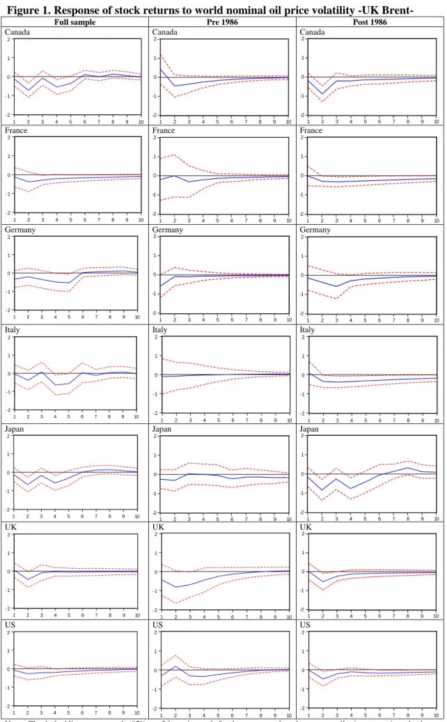
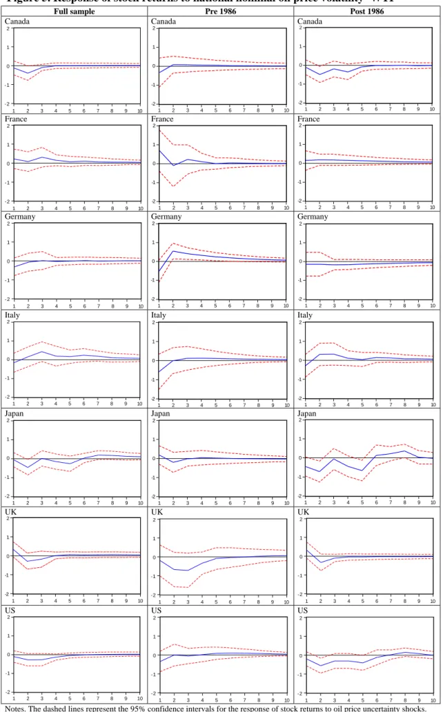
Figures 1 to 6 show the generalized impulse response functions of real stock returns to the following variables: world nominal -UK Brent- oil price volatility (Figure 1); national nominal -UK Brent- oil price volatility (Figure 2); national real -UK Brent- oil price volatility (Figure 3); world nominal -WTI- oil price volatility (Figure 4);

(10)

8

national nominal -WTI- oil price volatility (Figure 5); national real -WTI- oil price volatility (Figure 6). The dashed lines represent the 95% confidence intervals for the response of stock returns to oil price volatility shocks.

< Insert Figures 1 to 3 about here >

First, we find a significant change in how stock markets react to shocks in oil price volatility before and after January 1986. Oil price volatility has a larger negative effect on stock returns during the post-1986 period, except in the case of the UK (Figures 1, 2 and 6). These results are in accordance with Sadorsky (1999) who finds that, after 1986, oil price movements explain a larger fraction of the variance of stock returns.

Also, we can find a more significant effect of the UK Brent crude oil price volatility on G7 stock markets than that of WTI oil price.

The Canadian and Japanese stock markets are the most sensitive to oil price volatility. US and UK are less sensitive but still have diminishing stock returns related to higher oil price volatility. The French stock market reaction to changes in this volatility is mostly insignificant.

Canada is highly dependent on oil exports, and according to our findings, its stock market is more reactive to world oil price volatility, as shown in Figures 1 and 4, than it is to national real oil price volatility, as shown in Figures 2 and 5. We can also see in Figures 3 and 6 that the Canadian stock market shows a less significant reaction to real oil price volatility than it does to nominal oil price volatility.

Figures 1 and 4 also show that the French stock market only significantly reacts to a change in world oil price volatility, being most significant for the UK Brent crude (Figure 1). This structure of the French stock market corresponds to the post-1986 period, and consists in a negative reaction that is smoothly close to zero during 7 months.

In Germany, during the pre-1986 period, stock returns had an immediate reaction to oil price volatility change, recovering in the following period. For example, the German stock market presents a positive reaction to an increase in national nominal oil price volatility -WTI- for the pre-1986 period (Figure 5). Previous results are also in line with Cunado and Perez de Gracia (2013) who consider that the effect of oil price changes depend on the underlying cause of oil demand shock driven by the global economic activity. In the post-1986 period, this structure has changed into stock markets reacting mostly to nominal national oil price volatility.

In Figures 2, 3, 5 and 6, we can see that the Italian stock market shows a positive reaction to an increase in national oil price volatility. This is corrected when we use the world oil price volatility, as shown in Figures 1 and 4.Italy lacks energy resources and is entirely dependent on imports for its supply. In 1971, Italy introduced a floating exchange rate regime, and the reduction of oil prices through the devaluation of the lira enabled Italy to have an increase of exports, which have been central in the development of the Italian economy. This is a possible explanation of the positive stock return growth due to an increase in national oil price volatility, if oil price increases were in fact accompanied by the lira devaluation. However, when accounting for world oil price volatility, the Italian stock market does show a negative response in its returns.

(11)

9

On the other hand, Japan is also a large oil importer, and its stock markets show a significant effect due to changes in oil price volatility. Japanese stock market’s sensitivity to oil price volatility corresponds only to a post-1986 period, and shows to be higher for the UK Brent (Figures 1, 2 and 3) than it is for WTI (Figures 4, 5 and 6).

Figures 1 through 3 show that the British stock market suffers a significant negative effect due to a rise in Brent crude price volatility. It is less significant when referring to WTI price volatility (Figures 4, 5 and 6). Although the British stock market already had this response before 1986, the response became more significant during the post-1986 period. Its response also shows to be equivalent across different oil price specifications (world, nominal national and real national).

Finally, although the US is the largest oil importer, its stock market is usually highly diversified, and does not show a response to oil price volatility as significant as does the Japanese stock market (also a large importer). However, we can observe that in the post-1986 period, the US stock returns began having a negative response to increases in oil price volatility. This response is not as large as other G7 economies, but is still significant. The dynamic and magnitude of its response are similar across nominal (Figures 2 and 5) and real oil price volatility variations (Figures 3 and 6).

< Insert Figures 4 to 6 about here > 5. Concluding remarks

In this paper we analyzed whether changes in oil price volatility are captured by stock markets in the G7 countries using monthly data for the period 1970:01-2014:12. In order to estimate the impact of oil price volatility shocks on stock returns, we use an unrestricted VAR model including the following variables: short-term interest rates, economic activity, stock prices, and oil price volatility defined according to a GARCH (1, 1) model.

We consider alternative oil price specifications such as world, national and real prices expressed in both WTI and the UK Brent. Results indicate that world oil price volatility is generally more significant for stock markets than the volatility of oil price given in local currency. This is especially notable for Italy. These results are in line with Park and Ratti’s (2008), who find that the effect of oil price shocks are better captured by the UK Brent index, and not by a specification that reflects the offsetting movement in the exchange rate. In other words, we find that stock market behavior is more sensitive to the information given by indicators of oil prices itself, rather than its expected impact in local currency. Also, in accordance with findings from Hamilton (2008), we do not find much difference in using real or nominal oil prices for the volatility definition. Hamilton states that this is due to the fact that in most oil shocks, the change in nominal oil prices is larger than the overall change in general prices. Considering that inflation is generally controlled by monetary policy which reduces aggregate price volatility, the results of this paper reflect the larger impact of volatility of nominal oil prices than that of inflation in stock returns.

Jo (2014) finds that an oil price volatility shock has the immediate and persistent negative effect of lowering economic activity by about 0.1%-point. Under the idea that heightened volatility can deteriorate a variety of economic activity, the overall results of

(12)

10

this paper suggest that oil price volatility also has a negative effect on returns of the G7 stock markets. This implies that these markets are capturing the effect that oil price volatility has on economic activity, and expected returns are impacted by a higher volatility of the price of oil. In other words, the efficiency of stock markets should be higher when there is more certainty in the price of this major input. Similar results of a negative effect of oil price volatility in stock returns are found by Park and Ratti (2008). Also, Sadorsky (1999) stated that, after 1986, positive oil price volatility shocks explain a larger fraction of the variance of stock returns, suggesting a change in either the dynamics of oil price shocks or the structure of the economy. Cunado and Perez de Gracia (2005) also find the differential behavior before and after 1986, identifying large oil price declines and a heightened volatility. In our analysis, we use a GARCH (1, 1) model to define a time series for oil price volatility. In our empirical analysis, we can identify a heightened amount of volatility in oil prices in the post-1986 period. As the behavior of oil prices changed, the results of this paper show that G7 stock markets response to oil price volatility also changed. After 1986, G7 stock markets have reacted negatively to higher oil price volatility, which is not as significant in the pre-1986 period.

In light of these results, given that volatility of oil prices has been found to be relevant for predicting macroeconomic and financial variables, further research on this topic is needed. Additional research could focus on differential behavior, relative to price volatility, between oil importing and oil exporting countries. Also, this analysis could be extended to analyzing volatility of oil demand and oil supply shocks and to a micro-analysis at industry level.

(13)

11

References

Apergis, N., Miller, S., 2009. Do structural oil market shocks affect stock prices? Energy Economics, 31, 569-575.

Aye G., Dadam, V., Gupta, R., Mamba, B., 2014. Oil price uncertainty and manufacturing production. Energy Economics, 43, 41-47.

Caporale, G. M., Menla Ali, F., Spagnolo, N., 2015. Oil price uncertainty and sectoral stock returns in China: A time-varying approach. China Economic Review, 34, 311-321.

Chen, S. S., Hsu, K. W., 2012. Reverse globalization: Does high oil price volatility discourage international trade? Energy Economics, 34, 1634-1643

Cunado, J., Perez de Gracia, F., 2003. Do oil price shocks matter? Evidence for some European countries. Energy Economics, 25, 137-154.

Cunado, J., Perez de Gracia, F., 2005. Oil prices, economic activity and inflation: Evidence for some Asian economies. The Quarterly Review of Economics and Finance, 45, 65-83.

Cunado, J., Perez de Gracia, F., 2013. Oil prices shocks and stock market returns: Evidence for some European countries. Energy Economics, 42, 365-377.

Cunado, J., Jo, S., Perez de Gracia, F., 2015. Macroeconomic impacts of oil price shocks in Asian economies. Energy Policy, 86, 867-879.

Dickey, D. A., Fuller, W. A., 1981. Likelihood ratio statistics for autoregressive time series with a unit root. Econometrica, 49, 1057-1072

Driesprong, G. Jacobsen, B., Maat, B., 2008. Striking oil: another puzzle? Journal of Financial Economics, 89, 307-327.

Elder, J., Serletis, A., 2010. Oil price uncertainty. Journal of Money, Credit and Banking, 42, 1137-1159.

Elyasani, E., Iqbal, M., Odusami, B., 2011. Oil price shocks and industry stock returns. Energy Economics, 33, 966-974.

Federal Reserve Bank of St. Louis, 2015. FRED Economic Data, Spot oil price: West Texas Intermediate. <https://research.stlouisfed.org/fred2/series/OILPRICE> [15/03/2015].

Güntner, J. H., 2014. How do international stock markets respond to oil demand and supply shocks? Macroeconomic Dynamics, 18, 1657-1682.

Hamilton, J. D., 1983. Oil and Macroeconomy since the World War II. Journal of Political Economy, 91, 228-248.

Hamilton, J. D., 1996. This is what happened to the oil price-macroeconomy relationship. Journal of Monetary Economics, 38, 215-220.

Hamilton, J. D., 2003. What is an oil shock? Journal of Econometrics, 113, 363-398. Hamilton, J. D., 2008. Oil and the macroeconomy, In: Durlauf, Steven, Blume,

Lawrence (Eds.) New Palgrave Dictionary of Economics, 2nd edition. Palgrave McMillan Ltd.

Hamilton, J. D., 2011. Nonlinearities and the macroeconomic effects of oil prices. Macroeconomic Dynamics, 15, 364-378.

Herrera, A. M., Lagalo, L. G., Wada, T., 2011. Oil price shocks and industrial production: Is the relationship linear? Macroeconomic Dynamics, 15, 472-497. International Monetary Fund, 2015. International Financial Statistics.

<http://elibrary-data.imf.org/DataExplorer.aspx> [15/03/3015].

Jo, S., 2014. The effects of oil price uncertainty on global real economic activity. Journal of Money, Credit and Banking, 46, 1113-1135.

Johansen, S., Juselius, K., 1990. Maximum likelihood estimation and inference on cointegration with applications to demand for money. Oxford Bulletin of Economics and Statistics, 52, 169-210.

(14)

12

Kilian, L., Park, C., 2009. The impact of oil price shocks on the US stock market. International Economic Review, 50, 1267-1287

Lee, K., Shawn, N., Ratti, R. A., 1995. Oil shocks and the macroeconomy: the role of price variability. Energy Journal, 16, 39-56.

Miller, J. I., Ratti, R. A., 2009. Crude oil and stock markets: stability, instability and bubbles. Energy Economics, 31, 559-568.

Mork, K. A., 1989. Oil and the macroeconomy when prices go up and down: An extension of Hamilton’s results. Journal of Political Economy, 91, 740-744.

Narayan, P. K., Sharma, S. S., 2011. New evidence on oil price and firm returns. Journal of Banking and Finance, 35, 3253-3262.

Park, J., Ratti, R. A., 2008. Oil price shocks and stock markets in the US and 13 European countries. Energy Economics, 30, 2587-2608.

Phillips, P. C., Perron, P., 1988. Testing for a unit root in time series regression. Biometrika, 75, 335-346.

Sadorsky, P., 1999. Oil price shocks and stock market activity. Energy Economics, 21, 449-469.

Scholtens, B., Yurtsever, C., 2012. Oil price shocks and European industries. Energy Economics, 34, 1187-1195.

Sims, C.A., 1980. Macroeconomics and reality. Econometrica, 48, 1-48.

Pershin, V., Molero, J. C., Perez de Gracia, F., 2016. Exploring the oil prices and exchange rates nexus in some African economies, Journal of Policy Modeling, forthcoming.

US Energy Information Administration, 2015. Independent statistics & analysis, petroleum & other liquids. <http://www.eia.gov/dnav/pet/pet_pri_spt_s1_d.htm> [15/03/2015].

(15)

13

Table 1. Variable description and sources

Name Description Source

Stock returns Share prices, end of period International Financial Statistics

(International Monetary Fund)

Economic activity Industrial production index, seasonally

adjusted

International Financial Statistics (International Monetary Fund)

CPI CPI for all items, seasonally adjusted International Financial Statistics

Interest rates Short-term interest rate International Financial Statistics

Exchange rates Number of units of national currency per

US dollar, period average

International Financial Statistics (International Monetary Fund) and FRED Economic Data (Federal Reserve Bank of St. Louis)

Oil prices World nominal prices -UK Brent-

Nominal national price -UK Brent- Real national prices -UK Brent- World nominal prices -WTI- Nominal national prices -WTI- Real national prices -WTI-

FRED Economic Data (Federal Reserve Bank of St. Louis) and US Energy Information Administration

Notes. WTI is expressed in nominal oil price, US dollars per barrel. UK Brent is expressed in nominal oil price, US dollars per barrel.

(16)

14

Table 2. ADF and PP unit root tests

ADF test PP test

Level First difference Level First difference

(i) (ii) (i) (ii) (i) (ii) (i) (ii)

Economic activity Canada -2.113 -1.418 -4.669*** -7.018*** -2.521 -1.171 -25.410*** -25.370*** France -2.658 -1.651 -5.380*** -5.783*** -3.315 -1.481 -30.151*** -30.006*** Germany -3.159 -2.107 -30.121*** -30.338*** -2.866 -2.082 -29.218*** -29.534*** Italy -4.618*** -2.713 -4.551*** -5.339*** -4.280*** -2.182 -32.439*** -34.171*** Japan -2.868 -2.658 -13.443*** -13.488*** -2.887 -2.732 -23.718*** -23.634*** UK -6.278*** -3.456 -21.826*** -22.938*** -6.040*** -3.404 -23.123*** -23.089*** US -2.617 -1.697 -7.993*** -8.257*** -2.903 -1.887 -15.733*** -16.034*** Interest rates Canada -2.161 -3.035 -27.574*** -27.553*** -2.341 -3.377 -30.227*** -30.498*** France -1.558 -2.869 -18.600*** -18.589*** -1.589 -2.830 -18.509*** -18.497*** Germany -2.734 -3.450 -7.533*** -7.5217*** -2.106 -2.984 -21.855*** -21.852*** Italy -0.589 -2.073 -13.986*** -21.439*** -0.854 -2.188 -21.530*** -21.618*** Japan -1.872 -3.612 -7.435*** -7.4298*** -1.666 -3.159 -22.501*** -22.488*** UK -1.697 -2.205 -22.426*** -22.417*** -2.233 -2.843 -30.784*** -30.763*** US -1.525 -2.633 -10.431*** -10.441*** -1.439 -2.519 -15.130*** -15.132*** Stock prices Canada -1.046 -3.285 -17.294*** -17.303*** -0.939 -3.116 -17.307*** -17.313*** France -1.530 -2.369 -19.476*** -19.468*** -1.784 -2.672 -20.068*** -20.057*** Germany -1.077 -2.752 -21.028*** -21.022*** -1.353 -3.160 -21.071*** -21.065*** Italy -2.535 -2.959 -10.659*** -10.663*** -2.360 -2.730 -18.592*** -18.583*** Japan -1.992 -1.970 -16.659*** -16.650*** -1.932 -1.906 -16.595*** -16.583*** UK -1.277 -2.724 -19.094*** -19.086*** -1.291 -2.824 -19.175*** -19.166*** US 0.192 -1.955 -19.717*** -19.781*** 0.212 -2.019 -19.774*** -19.812*** Nominal oil prices -UK Brent-

Canada -2.079 -3.145 -15.686*** -15.669*** -1.630 -2.709 -15.617*** -15.600*** France -2.416 -2.526 -16.162*** -16.171*** -2.153 -2.267 -15.586*** -15.583*** Germany -2.500 -2.778 -16.416*** -16.404*** -2.176 -2.428 -16.309*** -16.297*** Italy -1.776 -2.298 -16.508*** -16.528*** -1.529 -2.057 -16.011*** -15.996*** Japan -2.665 -2.853 -15.960*** -15.945*** -2.129 -2.296 -15.835*** -15.819*** UK -1.690 -2.469 -16.659*** -16.639*** -1.361 -2.213 -16.613*** -16.594*** US -2.188 -3.041 -14.529*** -14.513*** -1.750 -2.637 -14.297*** -14.431*** Real oil prices -UK Brent-

Canada -2.720 -2.750 -17.672*** -17.663*** -2.499 -2.525 -17.649*** -17.640*** France -1.988 -2.840 -19.235*** -19.235*** -1.637 -2.482 -19.099*** -19.097*** Germany -2.703 -2.682 -18.407*** -18.399*** -2.413 -2.390 -18.274*** -18.265*** Italy -1.625 -2.883 -19.243*** -19.247*** -1.472 -2.711 -19.199*** -19.202*** Japan -2.657 -2.659 -18.352*** -18.334*** -2.492 -2.501 -18.341*** -18.324*** UK -2.599 -2.564 -19.584*** -19.572*** -2.246 -2.199 -19.454*** -19.441*** US -2.735 -2.754 -17.070*** -17.061*** -2.496 -2.515 -17.040*** -17.031*** Nominal oil prices -WTI-

Canada -2.227 -3.592 -15.520*** -15.504*** -1.529 -2.880 -15.608*** -15.592*** France -2.327 -2.442 -15.975*** -15.984*** -2.056 -2.169 -15.362*** -15.357*** Germany -2.633 -2.971 -15.847*** -15.835*** -2.269 -2.581 -15.803*** -15.791*** Italy -1.739 -2.085 -16.445*** -16.463*** -1.463 -1.958 -15.920*** -15.905*** Japan -2.758 -2.971 -15.388*** -15.372*** -2.321 -2.538 -15.467*** -15.452*** UK -1.805 -2.808 -17.162*** -17.142*** -1.592 -2.414 -17.111*** -17.092*** US -2.297 -3.353 -14.753*** -14.735*** -1.877 -2.851 -14.886*** -14.871*** Real oil prices -WTI-

Canada -2.770 -2.832 -16.516*** -16.507*** -2.526 -2.593 -16.574*** -16.565*** France -1.681 -2.466 -17.640*** -17.640*** -1.419 -2.190 -17.367*** -17.361*** Germany -2.608 -2.591 -16.946*** -16.937*** -2.332 -2.317 -16.868*** -16.858*** Italy -1.328 -2.483 -17.654*** -17.660*** -1.091 -2.248 -17.453*** -17.409*** Japan -2.640 -2.652 -16.650*** -16.632*** -2.483 -2.508 -16.585*** -16.567*** UK -2.461 -2.431 -18.287*** -18.274*** -2.182 -2.151 -18.270*** -18.257*** US -2.776 -2.820 -16.092*** -16.083*** -2.524 -2.577 -16.179*** -16.170*** Notes. (i) Constant; (ii) Constant and linear trend. *** means significant at 1%.

(17)

15

Table 3. Johansen and Juselius cointegration tests (variables: oil prices -UK Brent-, economic activity, interest rates and stock prices)

r = 0 r ≤ 1 r ≤ 2 r ≤ 3

(i) (ii) (i) (ii) (i) (ii) (i) (ii) World nominal oil prices -UK

Brent-Canada Trace statistic 50.307* 92.767* 18.676 33.381 8.327 14.566 2.847 5.109 Max-eigen statistic 31.631* 59.385* 10.348 18.816 5.481 9.456 2.847 5.109 France Trace statistic 59.171* 89.948* 17.580 33.015 8.648 18.930 3.015 5.617 Max-eigen statistic 41.590* 56.932* 8.932 19.086 5.633 8.312 3.015 5.617 Germany Trace statistic 73.532* 87.558* 16.699 28.608 7.408 12.005 2.152 3.170 Max-eigen statistic 56.834* 58.950* 9.291 16.603 5.256 8.835 2.152 3.170 Italy Trace statistic 58.662* 87.992* 22.936 44.246* 8.533 20.977 1.848 6.681 Max-eigen statistic 35.726* 43.746* 14.403 23.269 6.685 14.296 1.848 6.681 Japan Trace statistic 39.416 65.903* 18.149 33.242 9.736 14.012 2.258 5.728 Max-eigen statistic 21.267 32.661* 8.413 19.230 7.478 9.284 2.258 5.728 UK Trace statistic 60.095* 81.999* 22.105 38.719 7.255 19.404 1.651 5.601 Max-eigen statistic 37.990* 43.280* 14.850 19.314 5.604 13.803 1.651 5.601 US Trace statistic 31.059* 81.695* 14.738 26.774 6.340 11.805 0.662 4.093 Max-eigen statistic 16.321 54.921* 8.398 14.969 5.678 7.711 0.662 4.093 National nominal oil prices -UK Brent-

Canada Trace statistic 51.602* 94.283* 20.172 34.311 7.957 16.105 2.533 5.138 Max-eigen statistic 31.429* 59.972* 12.216 18.206 5.424 10.967 2.533 5.138 France Trace statistic 49.000* 91.163* 26.323 28.982 12.310 13.754 4.370* 5.493 Max-eigen statistic 22.678 62.181* 14.013 15.228 7.939 8.261 4.370* 5.493 Germany Trace statistic 65.641* 82.031* 16.901 25.884 8.355 10.839 2.270 3.055 Max-eigen statistic 48.740* 56.148* 8.546 15.045 6.084 7.783 2.270 3.055 Italy Trace statistic 71.957* 92.353* 32.958* 43.459* 16.121* 24.698 3.373 9.938 Max-eigen statistic 39.000* 48.893* 16.836 18.761 12.749 14.760 3.373 9.938 Japan Trace statistic 40.277 67.439* 20.001 34.253 9.807 14.125 2.704 5.055 Max-eigen statistic 20.276 33.186* 10.194 20.129 7.103 9.069 2.704 5.055 UK Trace statistic 57.095* 77.164* 19.918 33.076 6.068 18.245 1.233 4.684 Max-eigen statistic 37.177* 44.088* 13.850 14.831 4.835 13.561 1.233 4.684 US Trace statistic 31.059* 81.695* 14.738 26.774 6.340 11.805 0.662 4.093 Max-eigen statistic 16.321 54.921* 8.398 14.969 5.678 7.711 0.662 4.093 National real oil prices -UK Brent-

Canada Trace statistic 57.869* 100.707* 25.183 40.038 10.276 21.500 3.194 6.882 Max-eigen statistic 32.687* 60.669* 14.906 18.538 7.082 14.619 3.192 6.882 France Trace statistic 56.004* 93.110* 27.686 35.287 15.068 16.047 5.890* 6.846 Max-eigen statistic 28.318* 57.824* 12.617 19.240 9.179 9.200 5.890* 6.846 Germany Trace statistic 61.811* 80.356* 18.405 25.866 10.551 11.147 2.909 3.342 Max-eigen statistic 43.406* 54.490* 7.853 14.718 7.642 7.806 2.909 3.342 Italy Trace statistic 75.753* 100.044* 30.761* 49.519* 14.872 21.847 4.784* 7.174 Max-eigen statistic 44.991* 50.525* 15.890 27.672* 10.088 14.672 4.784* 7.174 Japan Trace statistic 42.464 69.328* 21.516 35.892 10.144 15.067 3.053 5.052 Max-eigen statistic 20.949 33.436* 11.372 20.825 7.091 10.015 3.053 5.052 UK Trace statistic 61.524* 78.710* 23.767 37.406 9.700 19.848 2.530 7.011 Max-eigen statistic 37.757* 41.304* 14.066 17.558 7.170 12.838 2.530 7.011 US Trace statistic 34.857 79.627* 17.439 29.828 8.510 13.938 0.794 5.350 Max-eigen statistic 17.418 49.799* 8.928 15.890 7.716 8.588 0.794 5.350 Notes. r denotes the number of cointegrating vector. * denotes rejection of the null hypothesis at the 10% level of significance. In column 3 (r = 0) we test the null hypothesis of no cointegration against the alternative of cointegration. (i) and (ii) mean exclusion or inclusion of a linear trend in the test equation, respectively. The AIC was used for the lag determination.

(18)

16

Table 3. (cont.) Johansen and Juselius cointegration tests (variables: oil prices -WTI-, economic activity, interest rates and stock prices)

r = 0 r ≤ 1 r ≤ 2 r ≤ 3

(i) (ii) (i) (ii) (i) (ii) (i) (ii) World nominal oil prices -WTI-

Canada Trace statistic 52.784* 95.441* 21.238 36.365 8.851 17.267 3.000 5.012 Max-eigen statistic 31.546* 59.076* 12.387 19.097 5.851 12.255 3.000 5.012 France Trace statistic 60.545* 84.809* 18.761 31.649 9.681 9.884 3.479 2.549 Max-eigen statistic 41.784* 53.160* 9.080 21.764 6.202 7.336 3.479 2.549 Germany Trace statistic 76.223* 91.219* 17.930 31.263 8.239 12.983 2.712 3.346 Max-eigen statistic 58.294* 59.956* 9.690 18.279 5.527 9.637 2.712 3.346 Italy Trace statistic 60.224* 93.917* 24.347 48.733* 9.248 21.587 2.135 7.041 Max-eigen statistic 35.877* 45.184* 15.098 27.146* 7.113 14.546 2.135 7.041 Japan Trace statistic 41.093 69.299* 18.701 35.204 9.935 14.531 2.299 5.781 Max-eigen statistic 22.392 34.095* 8.766 20.673 7.636 8.749 2.299 5.781 UK Trace statistic 62.463* 86.460* 24.464 42.298 7.762 19.934 1.919 5.769 Max-eigen statistic 37.999* 44.163* 16.702 22.364 5.843 14.166 1.919 5.769 US Trace statistic 32.962 90.360* 15.894 28.855 7.847 12.243 0.785 4.251 Max-eigen statistic 17.067 61.505* 8.048 16.613 7.062 7.992 0.785 4.251 National nominal oil prices -WTI-

Canada Trace statistic 54.346* 96.916* 22.993 37.576 8.440 19.334 2.686 5.046 Max-eigen statistic 31.353* 59.340* 14.553 18.242 5.754 14.288 2.686 5.046 France Trace statistic 49.642* 93.131* 25.972 27.600 11.904 13.506 4.278* 5.695 Max-eigen statistic 23.671 65.531* 14.067 14.094 7.626 7.810 4.278* 5.695 Germany Trace statistic 65.818* 82.540* 17.684 26.130 9.137 11.196 2.707 3.125 Max-eigen statistic 48.134* 56.410* 8.547 14.933 6.431 8.071 2.707 3.125 Italy Trace statistic 72.930* 93.696* 31.828* 42.930* 15.275 24.268 3.357 10.972 Max-eigen statistic 41.101* 50.766* 16.553 18.662 11.918 13.296 3.357 10.972 Japan Trace statistic 39.820 66.152* 20.237 32.875 10.157 13.965 2.592 5.340 Max-eigen statistic 19.582 33.277* 10.081 18.910 7.565 8.625 2.592 5.340 UK Trace statistic 59.359* 81.561* 22.164 36.351 6.700 18.795 1.606 5.078 Max-eigen statistic 37.195* 45.211* 15.464 17.556 5.094 13.718 1.606 5.078 US Trace statistic 32.962 90.360* 15.894 28.855 7.847 12.243 0.785 4.251 Max-eigen statistic 17.067 61.505* 8.048 16.613 7.062 7.992 0.785 4.251 National real oil prices -WTI-

Canada Trace statistic 54.916* 96.299* 24.052 38.328 9.398 20.131 3.027 5.985 Max-eigen statistic 30.864* 57.971* 14.654 18.197 6.371 14.146 3.027 5.985 France Trace statistic 48.004* 87.205* 24.905 28.322 13.858 14.744 5.092* 5.917 Max-eigen statistic 23.099 58.883* 11.047 13.578 8.766 8.827 5.092* 5.917 Germany Trace statistic 59.667* 79.177* 17.575 24.358 9.632 9.853 2.762 2.974 Max-eigen statistic 42.091* 54.819* 7.943 14.505 6.870 6.879 2.762 2.974 Italy Trace statistic 67.708* 91.867* 32.063* 48.591* 16.296* 22.248 4.472* 7.439 Max-eigen statistic 35.646* 43.276* 15.767 26.343* 11.824 14.810 4.472* 7.439 Japan Trace statistic 39.444 65.126* 20.692 32.721 10.180 14.157 2.699 5.293 Max-eigen statistic 18.752 32.404* 10.512 18.565 7.481 8.864 2.699 5.293 UK Trace statistic 59.536* 76.284* 22.473 34.287 7.651 18.922 2.004 5.611 Max-eigen statistic 37.063* 41.996* 14.823 15.365 5.647 13.311 2.004 5.611 US Trace statistic 34.222 80.150* 17.469 29.755 8.747 13.663 1.033 5.118 Max-eigen statistic 16.753 50.395* 8.722 16.092 7.714 8.545 1.033 5.118 Notes. r denotes the number of cointegrating vector. * denotes rejection of the null hypothesis at the 10% level of significance. In column 3 (r = 0) we test the null hypothesis of no cointegration against the alternative of cointegration. (i) and (ii) mean exclusion or inclusion of a linear trend in the test equation, respectively. The AIC was used for the lag determination.

(19)

17

Figure 1. Response of stock returns to world nominal oil price volatility -UK

Brent-Full sample Pre 1986 Post 1986

Canada Canada Canada

France France France

Germany Germany Germany

Italy Italy Italy

Japan Japan Japan

UK UK UK

US US US

Notes. The dashed lines represent the 95% confidence intervals for the response of stock returns to oil price uncertainty shocks.

-2 -1 0 1 2 1 2 3 4 5 6 7 8 9 10 -2 -1 0 1 2 1 2 3 4 5 6 7 8 9 10 -2 -1 0 1 2 1 2 3 4 5 6 7 8 9 10 -2 -1 0 1 2 1 2 3 4 5 6 7 8 9 10 -2 -1 0 1 2 1 2 3 4 5 6 7 8 9 10 -2 -1 0 1 2 1 2 3 4 5 6 7 8 9 10 - 2 - 1 0 1 2 1 2 3 4 5 6 7 8 9 10 -2 -1 0 1 2 1 2 3 4 5 6 7 8 9 10 -2 -1 0 1 2 1 2 3 4 5 6 7 8 9 10 -2 -1 0 1 2 1 2 3 4 5 6 7 8 9 10 - 2 - 1 0 1 2 1 2 3 4 5 6 7 8 9 10 - 2 - 1 0 1 2 1 2 3 4 5 6 7 8 9 10 -2 -1 0 1 2 1 2 3 4 5 6 7 8 9 10 -2 -1 0 1 2 1 2 3 4 5 6 7 8 9 10 -2 -1 0 1 2 1 2 3 4 5 6 7 8 9 10 -2 -1 0 1 2 1 2 3 4 5 6 7 8 9 10 -2 -1 0 1 2 1 2 3 4 5 6 7 8 9 10 -2 -1 0 1 2 1 2 3 4 5 6 7 8 9 10 -2 -1 0 1 2 1 2 3 4 5 6 7 8 9 10 -2 -1 0 1 2 1 2 3 4 5 6 7 8 9 10 -2 -1 0 1 2 1 2 3 4 5 6 7 8 9 10

(20)

18

Figure 2. Response of stock returns to national nominal oil price volatility -UK

Italy Italy Italy

Japan Japan Japan

UK UK UK

US US US

-2 -1 0 1 2 1 2 3 4 5 6 7 8 9 10 -2 -1 0 1 2 1 2 3 4 5 6 7 8 9 10 -2 -1 0 1 2 1 2 3 4 5 6 7 8 9 10 -2 -1 0 1 2 1 2 3 4 5 6 7 8 9 10 -2 -1 0 1 2 1 2 3 4 5 6 7 8 9 10 -2 -1 0 1 2 1 2 3 4 5 6 7 8 9 10 -2 -1 0 1 2 1 2 3 4 5 6 7 8 9 10 -2 -1 0 1 2 1 2 3 4 5 6 7 8 9 10 -2 -1 0 1 2 1 2 3 4 5 6 7 8 9 10 - 2 - 1 0 1 2 1 2 3 4 5 6 7 8 9 10 - 2 0 2 4 6 8 1 2 3 4 5 6 7 8 9 10 - 2 - 1 0 1 2 1 2 3 4 5 6 7 8 9 10 -2 -1 0 1 2 1 2 3 4 5 6 7 8 9 10 -2 -1 0 1 2 1 2 3 4 5 6 7 8 9 10 -2 -1 0 1 2 1 2 3 4 5 6 7 8 9 10 -2 -1 0 1 2 1 2 3 4 5 6 7 8 9 10 -2 -1 0 1 2 1 2 3 4 5 6 7 8 9 10 -2 -1 0 1 2 1 2 3 4 5 6 7 8 9 10 -2 -1 0 1 2 1 2 3 4 5 6 7 8 9 10 -2 -1 0 1 2 1 2 3 4 5 6 7 8 9 10 -2 -1 0 1 2 1 2 3 4 5 6 7 8 9 10

(21)

19

Figure 3. Response of stock returns to national real oil price volatility -UK

Italy Italy Italy

Japan Japan Japan

UK UK UK

US US US

-2 -1 0 1 2 1 2 3 4 5 6 7 8 9 10 -2 -1 0 1 2 1 2 3 4 5 6 7 8 9 10 -2 -1 0 1 2 1 2 3 4 5 6 7 8 9 10 -2 -1 0 1 2 1 2 3 4 5 6 7 8 9 10 -2 -1 0 1 2 1 2 3 4 5 6 7 8 9 10 -2 -1 0 1 2 1 2 3 4 5 6 7 8 9 10 -2 -1 0 1 2 1 2 3 4 5 6 7 8 9 10 -2 -1 0 1 2 1 2 3 4 5 6 7 8 9 10 -2 -1 0 1 2 1 2 3 4 5 6 7 8 9 10 - 2 - 1 0 1 2 1 2 3 4 5 6 7 8 9 10 - 2 - 1 0 1 2 1 2 3 4 5 6 7 8 9 10 - 2 - 1 0 1 2 1 2 3 4 5 6 7 8 9 10 -2 -1 0 1 2 1 2 3 4 5 6 7 8 9 10 -2 -1 0 1 2 1 2 3 4 5 6 7 8 9 10 -2 -1 0 1 2 1 2 3 4 5 6 7 8 9 10 -2 -1 0 1 2 1 2 3 4 5 6 7 8 9 10 -2 -1 0 1 2 1 2 3 4 5 6 7 8 9 10 -2 -1 0 1 2 1 2 3 4 5 6 7 8 9 10 -2 -1 0 1 2 1 2 3 4 5 6 7 8 9 10 -2 -1 0 1 2 1 2 3 4 5 6 7 8 9 10 -2 -1 0 1 2 1 2 3 4 5 6 7 8 9 10

(22)

20

Figure 4. Response of stock returns to world nominal oil price volatility

-WTI-Full sample Pre 1986 Post 1986

Italy Italy Italy

Japan Japan Japan

UK UK UK

US US US

-2 -1 0 1 2 1 2 3 4 5 6 7 8 9 10 -2 -1 0 1 2 1 2 3 4 5 6 7 8 9 10 -2 -1 0 1 2 1 2 3 4 5 6 7 8 9 10 -2 -1 0 1 2 1 2 3 4 5 6 7 8 9 10 -2 -1 0 1 2 1 2 3 4 5 6 7 8 9 10 -2 -1 0 1 2 1 2 3 4 5 6 7 8 9 10 - 2 - 1 0 1 2 1 2 3 4 5 6 7 8 9 10 -2 -1 0 1 2 1 2 3 4 5 6 7 8 9 10 -2 -1 0 1 2 1 2 3 4 5 6 7 8 9 10 -2 -1 0 1 2 1 2 3 4 5 6 7 8 9 10 - 2 - 1 0 1 2 1 2 3 4 5 6 7 8 9 10 - 2 - 1 0 1 2 1 2 3 4 5 6 7 8 9 10 -2 -1 0 1 2 1 2 3 4 5 6 7 8 9 10 -2 -1 0 1 2 1 2 3 4 5 6 7 8 9 10 -2 -1 0 1 2 1 2 3 4 5 6 7 8 9 10 -2 -1 0 1 2 1 2 3 4 5 6 7 8 9 10 -2 -1 0 1 2 1 2 3 4 5 6 7 8 9 10 -2 -1 0 1 2 1 2 3 4 5 6 7 8 9 10 -2 -1 0 1 2 1 2 3 4 5 6 7 8 9 10 -2 -1 0 1 2 1 2 3 4 5 6 7 8 9 10 -2 -1 0 1 2 1 2 3 4 5 6 7 8 9 10

(23)

21

Figure 5. Response of stock returns to national nominal oil price volatility

Italy Italy Italy

Japan Japan Japan

UK UK UK

US US US

-2 -1 0 1 2 1 2 3 4 5 6 7 8 9 10 -2 -1 0 1 2 1 2 3 4 5 6 7 8 9 10 -2 -1 0 1 2 1 2 3 4 5 6 7 8 9 10 -2 -1 0 1 2 1 2 3 4 5 6 7 8 9 10 -2 -1 0 1 2 1 2 3 4 5 6 7 8 9 10 -2 -1 0 1 2 1 2 3 4 5 6 7 8 9 10 - 2 - 1 0 1 2 1 2 3 4 5 6 7 8 9 10 -2 -1 0 1 2 1 2 3 4 5 6 7 8 9 10 -2 -1 0 1 2 1 2 3 4 5 6 7 8 9 10 -2 -1 0 1 2 1 2 3 4 5 6 7 8 9 10 -2 -1 0 1 2 1 2 3 4 5 6 7 8 9 10 -2 -1 0 1 2 1 2 3 4 5 6 7 8 9 10 -2 -1 0 1 2 1 2 3 4 5 6 7 8 9 10 -2 -1 0 1 2 1 2 3 4 5 6 7 8 9 10 -2 -1 0 1 2 1 2 3 4 5 6 7 8 9 10 -2 -1 0 1 2 1 2 3 4 5 6 7 8 9 10 -2 -1 0 1 2 1 2 3 4 5 6 7 8 9 10 -2 -1 0 1 2 1 2 3 4 5 6 7 8 9 10 -2 -1 0 1 2 1 2 3 4 5 6 7 8 9 10 -2 -1 0 1 2 1 2 3 4 5 6 7 8 9 10 -2 -1 0 1 2 1 2 3 4 5 6 7 8 9 10

(24)

22

Figure 6. Response of stock returns to national real oil price volatility

Italy Italy Italy

Japan Japan Japan

UK UK UK

US US US

-2 -1 0 1 2 1 2 3 4 5 6 7 8 9 10 -2 -1 0 1 2 1 2 3 4 5 6 7 8 9 10 -2 -1 0 1 2 1 2 3 4 5 6 7 8 9 10 -2 -1 0 1 2 1 2 3 4 5 6 7 8 9 10 -2 -1 0 1 2 1 2 3 4 5 6 7 8 9 10 -2 -1 0 1 2 1 2 3 4 5 6 7 8 9 10 - 2 - 1 0 1 2 1 2 3 4 5 6 7 8 9 10 -2 -1 0 1 2 1 2 3 4 5 6 7 8 9 10 -2 -1 0 1 2 1 2 3 4 5 6 7 8 9 10 -2 -1 0 1 2 1 2 3 4 5 6 7 8 9 10 -2 -1 0 1 2 1 2 3 4 5 6 7 8 9 10 -2 -1 0 1 2 1 2 3 4 5 6 7 8 9 10 -2 -1 0 1 2 1 2 3 4 5 6 7 8 9 10 -2 -1 0 1 2 1 2 3 4 5 6 7 8 9 10 -2 -1 0 1 2 1 2 3 4 5 6 7 8 9 10 -2 -1 0 1 2 1 2 3 4 5 6 7 8 9 10 -2 -1 0 1 2 1 2 3 4 5 6 7 8 9 10 -2 -1 0 1 2 1 2 3 4 5 6 7 8 9 10 -2 -1 0 1 2 1 2 3 4 5 6 7 8 9 10 -2 -1 0 1 2 1 2 3 4 5 6 7 8 9 10 -2 -1 0 1 2 1 2 3 4 5 6 7 8 9 10