NBER WORKING PAPER SERIES
BEST PRICES
Judith A. Chevalier
Anil K Kashyap
Working Paper 16680
http://www.nber.org/papers/w16680
NATIONAL BUREAU OF ECONOMIC RESEARCH
1050 Massachusetts Avenue
Cambridge, MA 02138
January 2011
The views expressed here are our own and not necessarily those of any institutions with which we
are affiliated, nor of the National Bureau of Economic Research. Kashyap thanks the Chicago Booth
Initiative on Global Markets for research support. We thank Cecilia Gamba, Aaron Jones, and Ashish
Shenoy for outstanding research assistance. We thank numerous seminar participants for helpful comments.
We are grateful to the Kilts Marketing Center and SymphonyIRI Group for the data. As a condition
of use, SymphonyIRI reviews all papers using their data to check that the data are not described in
a misleading fashion. However, all analyses in this paper based on SymphonyIRI Group, Inc. data
are the work of Chevalier and Kashyap, not SymphonyIRI Group, Inc.
NBER working papers are circulated for discussion and comment purposes. They have not been
peer-reviewed or been subject to the review by the NBER Board of Directors that accompanies official
NBER publications.
© 2011 by Judith A. Chevalier and Anil K Kashyap. All rights reserved. Short sections of text, not
to exceed two paragraphs, may be quoted without explicit permission provided that full credit, including
Best Prices
Judith A. Chevalier and Anil K Kashyap
NBER Working Paper No. 16680
January 2011
, Revised March 2011, Revised August 2012
JEL No. E3,E31,L11,L16
ABSTRACT
We explore the role of strategic price-discrimination by retailers for price determination and inflation
dynamics. We model two types of customers, "loyals" who buy only one brand and do not strategically
time purchases, and "shoppers" who seek out low-priced products both across brands and across time.
Shoppers always pay the lowest price available, the "best price". Retailers in this setting optimally
choose long periods of constant regular prices punctuated by frequent temporary sales. Supermarket
scanner data confirm the model's predictions: the average price paid is closely approximated by a weighted
average of the fixed weight average list price and the "best price". In contrast to standard menu cost
models, our model implies that sales are an essential part of the price plan and the number and frequency
of sales may be an important mechanism for adjustment to shocks. We conclude that our "best price"
construct provides a tractable input for constructing price series.
Judith A. Chevalier
Yale School of Management
135 Prospect Street
New Haven, CT 06520
and NBER
Anil K Kashyap
Booth School of Business
The University of Chicago
5807 S. Woodlawn Avenue
Chicago, IL 60637
and NBER
1
Introduction
We explore theoretically and empirically the importance of retailer price dis-crimination strategies for descriptions of price dynamics. We depart from the usual approach in the macro literature that ignores consumer heterogene-ity in the price-setting problem and instead make this heterogeneheterogene-ity central to the analysis. In particular, we posit that that some consumers are ac-tive shoppers who chase discounts, substitute across products in a narrowly defined product category, and potentially use storage to maintain smooth consumption whilst concentrating their purchases in sale weeks. Other cus-tomers are passive, and retailers will employ strategies to charge these two groups different prices. Due to the actions of these strategic consumers, we find that weighted average prices paid differ substantially from posted prices.
The model that we propose to account for this behavior is a model which does not necessarily speak to nominal price rigidities. But the model does suggest that conscious price discrimination rather than restrictions on the ability of firms to change prices (such as menu costs) is critical for under-standing price dynamics. In the context of our framework, the most natural way to understand nominal rigidities would be to look to the consumer side of the pricing problem rather than the firm side. But even without taking a stand on this issue, the evidence we develop does speak to a pair of debates that have emerged amongst macroeconomists looking at micro data.
For example, there is a measurement question of whether (and poten-tially how) intermittent price discounts, or “sales”, should be incorporated in price index construction. Since episodic sales occur quite frequently in some sectors, price series that ignore sale prices display infrequent price changes, while price series that contain sales prices display very frequent price changes. Nakumura and Steinsson (2008) estimate a median price du-ration of approximately 5 months including sales, and approximately 8 to 11 months excluding them. Klenow and Kryvtsov (2008) find that consid-ering only regular (e.g., non-sale) prices raises the estimated median price duration in their dataset from 3.7 months to 7.2 months. In general, many researchers have documented that the price series for a given product from retailers such as grocery stores exhibit long periods of a constant regular price punctuated by occasional sales. These measurement issues come to the fore when macroeconomists must decide how to calibrate models that presume that prices are sticky. Our empirical analysis argues strongly for keeping track of sale prices because they play a major role in governing stores’ profits and our model suggests that their depth and/or frequency
could be altered to adjust to shocks.
Likewise, a largely theoretical literature has emerged to look at the micro-foundations for why sales exist. For example, Matejka (2010) builds on the literature of rational inattention (see Sims (1998, 2003), Mankiw and Reis(2002,2006), for example) to explore its implications for price setting. In his model firms do not know the exact cost of the good each is selling and the firms find it expensive to keep track of all the information that would be necessary to perfectly deduce this cost. Thus, firms must decide which cost signals to monitor and because of their finite processing ability will set prices based on the estimated distribution of cost. In order to economize on information, the seller chooses signals that lead to a small number of distinct prices. Sales in this framework corresponding to situations in which a signal suggests that costs were low.
There is a complementary long literature, beginning with Varian (1980) and Sobel (1984) that rationalize price-discrimination strategies that include temporary discounts. Guimaraes and Sheedy (2011) were the first to bring this perspective to the macroeconomic literature on price-setting. Like us, they assume heterogeneous consumers. They have two types of consumers, bargain hunters and loyal shoppers, who are price insensitive; they explore how price discrimination plays out when retailers compete to sell to these customers. The key finding in their analysis is that competition bounds the importance of sales as a mechanism to adjust to shocks.
Interestingly, the theoretical results in Guimaraes and Sheedy (2011) contrast the empirical results of Klenow and Willis (2007), who find that sale prices are just as responsive to macroeconomic conditions as regular prices. That is, Klenow and Willis find that the depth of sales decreases when recent inflation has been high and that sales prices give way to higher regular prices when recent inflation has been high.
Our contribution is largely empirical, but to guide the analysis we begin by introducing a model in the spirit of Varian (1980), Sobel (1984), and Pe-sendorfer (2002) that allows for the possibility that pricing strategies might involve variation in the usage of discount prices. In contrast to the previous literature, we focus explicitly on a retailer controlling the prices of multiple products. The robust implication of this kind of model is that store pricing patterns ought to reflect the presence of different consumers and be strate-gically coordinated across products. The model can account for frequent temporary sales and long periods of constant regular prices. Furthermore, even with unchanging costs and demand, optimal markups are not held con-stant across items or across time. In contrast to Guimaraes and Sheedy, our model also implies that changing the frequency and depth of sales is the
optimal response to cost shocks and to certain kinds of demand shocks. To quantify the importance of consumer heterogeneity we turn to de-tailed microeconomic data. Some of our data are for particular supermar-ket products collected over parts of seven years at Dominick’s Finer Foods (DFF), a supermarket chain in the Chicago area. We also analyze data for a later seven-year period, using a dataset provided by Symphony IRI. The IRI dataset covers stores in 47 markets around the country and we (randomly) selected one store in each of the nine census regions for evaluation. Prices for individual products at DFF and at the IRI stores display the now-familiar pattern of very infrequent regular price changes combined with frequent temporary sales. But upon more careful scrutiny, it appears that purchase patterns associated with the sales clearly reflect the important role played by bargain hunters. In particular, we show three sets of results.
First, the model suggests that average prices paid for goods within a bundle of close substitutes are the relevant price for consumers and retailers. Because retailers time sales strategically, the model suggests, and the data show, that sales for close substitute products tend not to occur in the same weeks. Consumers, we show, chase sales, and thus, actual prices paid are substantially lower than regular prices, and even measurably below average posted prices.
Second, we introduce the concept of a “best price”, defined as the lowest price charged for any good in the narrow product category during a short multi-week time window. The model predicts that “best prices” should be the relevant prices for sales-chasing consumers. We show that the actual price paid tracks the “best price” and is well-approximated by an average of the best price and the fixed weight price index. The data match the structural form of our model.
Third, the data exhibit strong spillovers in quantities purchased due to price changes for close substitutes. So, for example, when the price of Minute Maid orange juice is reduced for a temporary discount, sales of Tropicana orange juice plunge (provided the Tropicana price does not change). In previous literature, large quantity variation along with constant prices has lead to a diagnosis of substantial demand variability. However, we show that much of this apparent demand volatility derives from choices made by the retailer in setting prices for substitute products. For example, we show that total ounces sold of all products within a narrow product category are much less volatile than total ounces sold of any individual product suggesting that while customers actively shift between items when they go on sale, making individual demand quite volatile, the total demand across all the relevant items is much more stable.
We read the evidence as suggesting that the models of price setting that emphasize consumers taste, cognitive processing, or information-gathering deserve more attention. For instance, in our model, occasional sales provide a tool for retailers to effectively charge different consumers different prices and pricing decisions are driven by the different consumer groups’ reservation prices. Thus, how consumers update reservation prices for individual goods becomes a critical factor affecting inflation. This mechanism has been much less explored than have those which emphasize firms costs of changing prices. Similarly, price index construction may need to be revised to account for the importance of bargain hunters. We provide some preliminary thoughts on how this might be done.
Our paper proceeds as follows. Section 2 provides the simple model of a price-discriminating retailer and highlights empirical predictions. Section 3 describes the data. Section 4 establishes a number of new facts about pricing and purchase patterns that are consistent with the model. Section 5 discusses how to use our model to measure and summarize price series. Section 6 concludes.
2
A Model of Price Discriminating Retailers and
Heterogeneous Consumers
We begin by presenting a simple model that is similar in spirit to, and bor-rows significantly from, Varian (1980), Sobel (1984), or Pesendorfer (2002). The baseline version of our model takes consumer heterogeneity as its prim-itive. The firm knows about this heterogeneity and accounts for it in price setting. In this model, the firm bears no menu cost of changing prices. Nonetheless, we will show that the firm will iterate between a small number of prices, even in the face of some cost changes and some types of demand changes. The “regular” price will change infrequently but “sales” will be utilized. The model suggests that it is possible that the retailer will respond to a nominal shock by changing the frequency of sales while holding the “regular” price fixed.
2.1 Model Assumptions
Consider a retailer selling two substitute differentiated products, A and B. We will focus on a single retailer for simplicity. However, we note that it would be fairly straightforward to embed our model into a model of two retailers competing in geographic space. In such a model (see, for example,
Lal and Matutes (1994), Pesendorfer (2002) and Hosken and Reiffen (2007)), consumer reservation prices would be determined by the price that would trigger consumer travel to another store. Thus, for tractability, we focus on a single retailer, but a monopoly assumption is not necessary. We discuss the competitive case more below.
Assume that all customers have unit demand in each period but are differentiated in their preferences for the two substitute goods. A share α/2 of the customers value product A at VH and product B at VL, where VH > VL. We call these consumers the high A types. For convenience, we consider the symmetric case where a shareα/2 of the customers, the high B types, value product B atVH and product A atVL. The remaining share of consumers (1−α), the “bargain hunters”, value both products at VL. We normalize the total number of consumers to be 1 and considerN shopping periods.1
The seller has a constant returns to scale technology of producing A and B and the marginal cost of producing either isc.
Each period, customers arrive at the retailer to shop. Consider the choices for the high A types (which will be symmetric for the high B types). If the price is less than or equal to their reservation value (PA< VH), then they buy their preferred good, A. IfPA> VH and the price for product B is less than or equal to their reservation price for B (PB < VL), the high A type customers substitute to good B. If PA > VH and PB > VL, then the high A types make no purchase. For simplicity we also assume that, if the high types do not buy, their demand for the period is extinguished so that next period there are no implications of them having been out of the market.2
Next consider the choices made by the bargain hunters. If PA < VL and/orPB < VL, they will buy whichever product is cheaper.3 IfPA> VL
andPB> VL, the bargain hunters do not buy. However, we capture the idea of shoppers being willing to engage in intertemporal storage by assuming that their demand partially accumulates to successive periods, deteriorating at rate 1-ρ. Thus, for example, if they made a purchase in period t−1,
1
In our model,VH andVLare real. However, it is possible that one or both types of consumer have nominal illusion. This would influence the retailer’s optimal response to changes in monetary policy. We leave exploration of this set of issues to future work.
2In our model, as long as costs are less than VH, the firm will always set price so
that the high types purchase. We could make an assumption about high type demand accumulating, but it wouldn’t have any important implications for the model.
3
We will see that in equilibrium it will not be profit maximizing to put both goods on sale in the same week.
butPA=PB =VH in periodt so that no purchases are made, then their total demand entering period t+ 1 will be (1−α) + (1−α)ρ. Similarly, if a good was available at a price ofVL in periodt−1, butPA=PB =VH
in periods t,t+ 1, . . . , t+ (k−1), total demand from the bargain hunters in period k will equal:
(1−α)(1 +ρ+ρ2+· · ·+ρk) = (1−α)(1−ρ
k)
1−ρ if 0< ρ <1. Note then, that we are assuming that the high types are inactive shoppers —they do not wait for and/or stock up during bargains, while the low types do. In this sense, our model reflects well the empirical facts described in Aguiar and Hurst (2007), in which they document that some consumers in a local area pay systematically lower prices for the same goods as other consumers. That is, some consumers are strategic in bargain-hunting, and others are not.4
Total profits for the retailer depend on the total amount of A and B sold. The retailer has three basic choices: (i) the retailer can charge high prices and service only the high types, foregoing any potential margins to be earned on the low types. (ii) the retailer can charge low prices and serve both types of customers, thus foregoing the extra willingness to pay that could have been extracted from the high types. Or (iii) the retailer can strategically iterate between high and low prices in an attempt to capture some of the potential demand from the bargain-hunters while exploiting some of the extra willingness to pay of the high types.
2.2 Model Results
Depending on the parameters, strategy (i), (ii), or (iii), described above can be optimal. We will explain when each is optimal, with particular attention to parameter values under which (iii) is optimal, since the pricing behavior associated with (iii) is roughly consistent with our empirical observation of occasional sales at supermarkets. We characterize the retailer’s behavior in several steps.
Proposition 1: As long as VL > c, the optimal price in any period is eitherVL orVH.
4As in Pesendorfer (2002), we combine “bargain-hunting” behavior with low willingness
to pay. We could provide a more detailed model with more types—brand loyals who are willing to intertemporally substitute purchases, brand loyals who do not intertemporally substitute, non-loyals who are willing to intertemporally substitute and non-loyals who do not intertemporally substitute. We think most of the interesting implications are evident with these 4 types collapsed into the two extremes.
Sketch of Proof: Choosing a price between VH and VL would reduce margins on the high types but would produce no offsetting demand increase for the bargain hunters. Thus, the optimal price is eitherVH orVL.
Proposition 2: It is never optimal to charge VL for both good A and good B in the same period.
Sketch of Proof: Charging VL for the second good leads to a loss of margins on the high types that prefer that good, but produces no offsetting demand increase for the bargain hunters. The bargain hunters’ demand is satisfied by chargingVLforeither good. This delivers one of the prediction that we will test empirically, namely that discount periods or “sales” for products within a product category are not synchronized.
Thus, we have shown that the retailer will charge VH for at least one good in every period, and may charge VL for one good in some periods. Below, we show the conditions under which the retailer will charge VL for one good in every period, conditions under which the retailer will never charge VL for either good, and conditions under which the retailer will charge VL for one good in some periods but not all periods (intermittent sales). In order to derive these results, we first provide two straightforward intermediate results.
Proposition 3: If the retailer chooses to hold one and only one sale during the N periods, then the optimal time to hold it will be in the Nth (final) period.
Sketch of Proof: If the retailer charges VH for both products during N−1 periods, andVL for one product in 1 period, profits will be:
(N −1)α(VH−c) +α 2(V L−c) +α 2(V H −c) + (1−ρk) 1−ρ (1−α)(V L−c) (1)
wherekrepresents the period in which the sale is held. The first term of (1) is the profits from the high types in all of the non-sales periods, the second and third term represent the profits from the high types in the sale period (if the sale is on A, the high A types pay VL, but the high B types still pay VH). The fourth term of (1) represents the profits from the bargain hunters. Note that the first three terms are invariant to the timing of the single sale. The fourth term is maximized whenk=N (as long asρ >0).
Proposition 4; For a retailer who chooses to hold j sales (i.e. chargeVL in j periods), the optimal strategy is to hold evenly spaced sales every k periods, wherek=N/j.
Sketch of Proof: The prior proposition covered the case of j = 1 and k= N. Note that the logic underlying Proposition 3 for the entire period carries forward straightforwardly to sub-periods, so within each sub-period it makes sense to delay the sale as long as possible. Hence sales will be equally spaced.
With the results of Propositions 3 and 4 in hand, we can characterize the remaining decision about when it pays to have any sales at all. We consider a retailer who holds a sale everykth period. If k= 1, the retailer holds a sale every period. Ifk=N, the retailer holds the minimum positive number of sales—one sale at the end to “sweep up” the low demanders. If k > N, the retailer never holds sales. We will focus on interior solutions where 1< k < N.
We consider the profits of a retailer who chargesPA=PB =VH every period except during a “sale” and holds a sale at P = VL for one or the other good everykth period. Assuming no discounting, total profits for this retailer over allN periods are:
Nk−1 k α(V H −c) +N k α 2(V L−c) +N k α 2(V H −c) + N k (1−ρk) 1−ρ (1−α)(V L−c) (2)
The four terms in (2) are very intuitive. The first piece represents the profits from selling to the high types only, which will occur during all the non-sale periods. The second term is the profits from the high types during the periods where they are able to buy their preferred good on sale; during these sale periods the other high type still pays VH so that explains the third term. The last term is the profits from the bargain hunters. Note that, the larger ρ is, the less the bargain hunters’ demand has depreciated by the time the sale is held.
Proposition 5: The retailer will find it optimal to hold some sales if: α 2(V H −VL)<(1−α)1−ρN 1−ρ (V L−c)⇔ VH < VL+ 21−α α 1−ρN 1−ρ (V L−c) (3)
Sketch of Proof: The left hand side of first expression shows the loss from allowing the high types to pay less than they are willing to pay by offering a single sale. The right hand side of the first expression gives the profits from selling to the bargain hunters in an optimally timed single sale.
The second expression in (3) helps build intuition. Essentially, holding at least one sale will be optimal as long as VL is large “enough” relative to c and relative toVH and if there are enough bargain hunters. The total
demand of the bargain hunters depends on both their share in the population and the extent to which their unmet demand cumulates. An increase in the share of bargain hunters (or increase the persistence of their demand) will lead to more sales.
Note also that, if the stock of consumers depreciates completely (ρ= 0) from period to period, then the condition degenerates to the condition for profits from charging the low price being higher than profits from charging the high price (period by period):
α 2(V H −c)<1−α 2 (VL−c)
Assume that the condition in Proposition 5 holds so that the retailer will hold at least 1 sale. By construction, for given values ofα,ρ,VH,VL, and c, the seller will then choose k to maximize (2). That is, the seller will deterministically hold a sale everykth period. We are assuming thatk and N are positive integers. However, we can examine comparative statics involving the optimal choice ofk by treating these functions as continuous and maximizing profits with respect tok. We are considering the cases here whereN is large.
With profits given by (2), the first order condition fork is:
k= 1 logρ × 1 +W α(VH −c)−(2−α)(VL−c)−αρ(VH −VL) 2e(1−α)(VL−c) (4)
WhereW(·) is the Product Log or Lambert function. The Lambert function provides the solution forzsuch thatz=W(z)eW(z). It is used extensively
to model time delay problems in operations research—a family of problems akin to the timing of sales problem studied here. Note that, since k is the number of periods between sales, a larger kmeans less frequent sales.
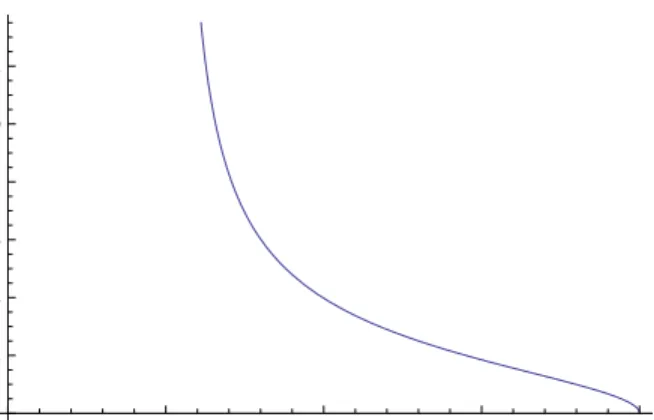
While analytic solutions are unavailable, by fixing some parameters we can present a few interesting and illustrative comparative statics numerically. For example, consider the case where VH = 4, c = 1, ρ = 0.9, α = 0.4.
Figure 1 shows the optimalk forVL varying from 0 to 4.
Not surprisingly k is decreasing in VL: the higher the valuation of the low valuation types, the shorter the time between sales; serving the low
valuation types is attractive. Note that k is not defined if VL is too low, because at some point it ceases to make sense to have sales. Also, note that as VL → VH = 4, the optimal k falls below 1. That is, as VL gets large
enough, it makes sense to charge VL for one product every period.
Alternatively consider the effect of c on the optimal k. Fix VH = 4, ρ= 0.9, α = 0.4 as before, and fix VL = 2. Figure 2 shows that, as would be expectedk is increasing inc: the greater is marginal cost, the lower the profits from serving the bargain hunters and the less frequently one would want to hold sales. Asc→VL= 2,k→ ∞.
Given the structure of our model, the firm is always charging VH when there is not a sale. So changes in marginal cost that are unaccompanied by changes in buyer willingness to pay will not result in a change in the non-sale price.
Lastly, consider changes in α, the share of customers with high willing-ness to pay for one of the goods. As before, fix VH = 4, VL = 2, c = 1, and ρ = 0.9. Figure 3 shows the optimal k asα ranges from 0 to 1. As α increases, i.e. the share of bargain hunters falls, sales become less attractive. Ifα= 1, optimal kis infinite, because sales are never attractive.
From the retailer’s point of view the relevant “price plan” is the full se-quence of high and low prices that prevail over the cycle of 2kperiods. Note that even with unchanging cost and demand parameters, for many param-eter values, the firm changes prices from period to period as it optimally iterates between capturing rents from high types and capturing the demand of the “bargain hunter” low types. Fixing tastes and technology in this set up, the main choice variable of the retailer isk. PA and PB are choices in each period but are set by the willingness to pay of the consumer types.
It is useful to compare the outcomes of this model to the models proposed in Kehoe and Midrigan (2010) and Eichenbaum, Jaimovich, and Rebelo (2011). Both of those models can produce a result of a firm charging a fixed regular price and sometimes charging a sale price. However, in both of these papers, the decision to charge a sale price is driven by some change in the cost or demand environment. In our model, a sale would occur every kweeks with no change in the cost or demand environment.
It is also useful to compare this model to Pesendorfer (2002), the mi-croeconomic model that ours most closely resembles. In Pesendorfer, the sale decision is stochastic, but shocks to cost are an important driver of the decision to hold a sale.
Another important distinction between all of these models and ours is that none of these models explicitly examine a retailer managing a portfolio of close substitute products. Indeed, the fact that cost drivers are important
in these models implies that the prices for close substitute products would tend to be positively correlated. In our model, the time series of prices for close substitute products arenegatively correlated (unless a common shock leads to the change inVL and VH).
Guimaraes and Sheedy (2011) share the feature of our model that sales are not driven primarily by cost shocks. Their model, like Sobel (1984), examines two competitors (competing brands or competing retailers) chasing a fixed pool of bargain hunters. They do not examine a single retailer managing a portfolio of close substitute products. In their model, sales will not be negatively correlated across competing brands.
It is also useful to enumerate the circumstances in our model that would lead to a change in the regular price. The regular price is held constant if there are shocks to any of the following parameters: VL,c,ρ, andα. If any of those parameters change, the retailer’s optimal response is to alter the frequency or depth of sales.
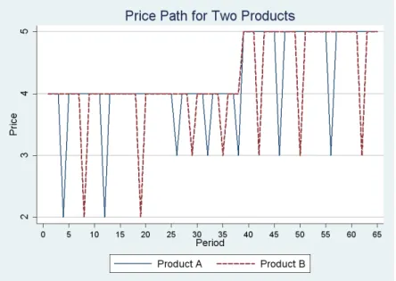
One way to combine the comparative statics described above is to sim-ulate the model allowing for changes in preferences and costs, under the assumption that the seller expects each change to be permanent. In the following figure we fix the persistence of unmet demand, but allow the share of the bargain hunters, the valuations of the bargain hunters and high types, and marginal cost to each change once per quarter. In this experiment the taste/cost shocks occur every thirteen weeks.
A resulting price path from this simulation for good A is plotted in Figure 4. Having allowed for a full set of shocks, the model now predicts changes in prices, the frequency of sales and the size of the discount that occurs during a sale. While our model is highly stylized, the price pattern from our simulation in Figure 4 does look extremely similar to a price series for substitute grocery products.
Finally, it is helpful to use the model to think about quantities sold. In the simplest case where demand does not deteriorate at all from period to period but just stockpiles (ρ = 1), total units purchased over all periods equals N, independent of the number and frequency of sales. This follows literally from the assumption of unit demand per period. But even so, the number of units sold in each individual period, however, is a function of the timing of sales; bargain hunters move all of their demand into sale periods. The only distortion in total units purchased over all N periods relative to the scenario in which PA = PB = VL in all periods stems from the
deterioration in bargain hunter demand while waiting for sales. Thus, for generalρ, total units sold equal =N α+N
k
(1−ρk)
Note that, in any individual period, sales of an individual good could be as low asα/2 and as large asα+k(1−α), if the good is on sale and deterio-ration of “bargain hunter” demand is negligible. Note that this volatility in demand across products and periods occurs despite the static environment that we modelled; quantity sold varies across periods and across goods de-spite the fact that the demand and supply primitives are constant through time. This implies that, while individual good sales are volatile period by period, by summing across goods A and B the total amount sold will be in-variant acrossk-period cycles. Building on this prediction, we look whether the volatility in quantities sold are smaller for a collection of close substi-tutes over a full cycle of weeks that include at least one discount, than in individual weeks or for individual goods.
The preceding results are also helpful for thinking about actual prices paid. Summing over all periods and the products A and B, VH will be the price charged in at least half of the product-periods. In cases in which there are interior solutions for k (as depicted above), VH will be the price charged in more than half of all product-periods. Specifically, if A and B are discounted equally frequently, the share of periods in which a given product is “on sale” is 1/2k. Thus, applying the algorithms proposed by either Eichenbaum, Jaimovich and Rebelo (2011) or Kehoe and Midrigan (2010) would identify VH as the regular/reference price for both goods. A “fixed weight” index measuring average price over the entire period would measure an average price of:
1 2kV
L+2k−1
2k V
H (5)
This price (and certainly the “regular” price) does not capture aver-age price from the retailer’s perspective or from the perspective of the bargaining-hunting customer. The actual price paid puts much more weight on the low price, because it reflects the strategic shift of the bargain-hunters into the low priced product (when one is on sale) and the stockpiling of bargain hunter demand (when nothing is on sale).
This is easiest to see by first neglecting/assuming away the deterioration in bargain hunter demand. With no demand deterioration, average revenue per unit equals:
α+ 2k(1−α)
2k V
L+α(2k−1)
2k V
H (6)
Of course, we know that lower prices expand demand, but in this case, that factor is magnified by the presence of multiple products that bargain
hunters view as substitutes and because bargain hunters stockpile demand. It will be very helpful to note the relationship between (5) and (6). Recall that (5) is the fixed weight index and that (6) is the average revenue per unit or actual price paid. Note also that the lowest or “best price” achieved over the k period sales cycle is VL. The average price paid in (6) can be rearranged to be equal to:
α 1 2kV L+2k−1 2k V H + (1−α)VL (7)
That is, the actual price paid in (6) is equal a weighted average of the fixed weight price index in (5) and the “best price”, where the share of loyals and of bargain hunters in the population are the weights.
The average revenue per unit (or actual price paid per unit) is more complicated when demand deterioration is taken into account. The weighted average price then becomes:
α 2k + (1−α)(1−ρk) k(1−ρ) VL+α(2k−1) 2k V H α+(1−α) k 1−ρk 1−ρ (8)
The average revenue in (8) approaches that in (7), or equivalently (6), as ρapproaches 1. Forρ <1, the weighted average price in (8) is slightly higher than in (6) because demand deterioration destroys some of the demand when sale prices are not offered. Thus, the average revenue per unit, or actual price paid, is a weighted average of the price paid by the high types, and the price paid by the low types.
Note also from (8) that, ifρis small, then asαapproaches 0, the weighted average price will approach the “best price”—the lowest price posted for any of the substitute products within thekperiod planning cycle. Note also that ifα is fairly small and ifρis small andVH remains constant for a long
period of time, then a time series of the weighted average price will resemble a fixed increment over the time series of the “best price”. Ifα is very large, then the weighted average price will more closely resemble the “regular” or “reference” price. For small to modest values ofρ and intermediate values of α, the price paid resembles a weighted average of the “best” price and the fixed price index as illustrate in (7). We examine these possibilities in the next section.
Our model is highly stylized and so we discuss ways in which it may be extended. First, the model extends straightforwardly to more substitute
goods. One can imagine more complex demand relationships that could be exploited by the retailer. For example, in our model, each product is associated with a cadre of brand-loyal consumers. However, it is possible that the retailing landscape includes some goods for which some consumers are brand loyal and other goods for which no consumers are brand loyal (possibly private label goods).
Furthermore, there are numerous ways to contemplate an extension of the model to multiple types. In particular, as mentioned above, there may be some consumers who inter-temporally substitute actively, but are highly brand loyal. There may be other consumers who are not brand loyal but do not inter-temporally substitute. In these more complex cases, the for-mulation and intuition in (6) is particularly helpful. Specifically, we can think of the prices paid for a set of closely related goods over a shopping cycle as being characterized by the weighted average of the prices paid by non-bargain hunter loyal shoppers and the prices paid by bargain hunters. As shown above, the prices paid by the loyal shoppers are essentially a fixed weight average of the prices posted. However, the prices paid by bargain hunters more closely resemble the lowest price charged for any substitute good over a reasonable shopping horizon. In a model with more types, the pricing outcomes will be as in (6) but the weights on the different prices will reflect the behavior of the different consumer types.
Also, while there is a long tradition of two-type models in the literature on temporary discounts (including Varian (1980) and Sobel (1984)) exten-sion to a continuum of consumer willingnesses to pay is possible. As in Varian (1980), as long as enough consumers are not adept at moving all of their purchases into sale periods, intertemporal variation in prices will enhance the retailer’s ability to price discriminate.
Our model also abstracts from competition among multiple stores. Ob-viously, a model with perfect competition would limit the opportunity to price discriminate. However, an extension of our model along the lines of Lal and Matutes (1994) should preserve the basic insights of our model. Lal and Matutes (1994) model multiproduct retailers with travel costs between stores. The ability of consumers to shop both stores, at a cost, disciplines the overall rents across products that stores can extract from each consumer. However, the ability to extract different levels of rents from different con-sumer types and from different products is preserved. Ellison (2005), in a different context, provides an extension of Lal and Matutes in which price discrimination across consumer types emerges in an equilibrium with spa-tial competition. The easiest way to understand the effects of introducing competition into our model is to view competition as impacting consumer
willingness to pay. Spatial competition opens additional scope for price discrimination as retailers may benefit from price discriminating between consumers who will and won’t travel to obtain a price discount.
While our model is stylized, it provides a useful framing for our analysis. Below, we will show empirically that the prices paid in our data resemble a weighted average of a fixed weight index and the “best price”, as in (6). We use these insights to speculate about pricing implications in more com-plicated environments than those described by the model and we provide a preliminary discussion of approaches to measuring and characterizing prices in such environments.
Summing up, the model comfortably explains the familiar price pattern observed for individual goods of a regular price with intermittent sale prices. In addition, it makes the following testable predictions. First, sales across items should be staggered. Second, demand will be more stable for bundles of close substitutes across several weeks (that include at least one sale) than for individual weeks or for individual items over that same period. Third, the actual price paid will be much lower than a regular or normal price if bargain hunters are important. Fourth, prices paid should generally be a combination of a conventional fixed weight price index and the best available price within the group of close substitutes over the course of several weeks. Finally, it is possible that the frequency of sales (or the size of discounts) will be a meaningful margin of adjustment in a pricing strategy. More generally, the updating rules that consumers use in revising their reservation prices will play a critical role in determining prices.
3
The Data
Given our interest in examining both the incidence of sales and consumer responses to them, our project requires a data set that contains both prices and quantities. This eliminates many data sets, most notably those from the Bureau of Labor Statistics that have been the source for many of the most important recent papers on price setting patterns. We instead we rely on two scanner data sets (from Dominick’s and IRI Symphony) that include quantity information.
The data for two of the categories we analyze are taken from Dominick’s Finer Foods (DFF). DFF is a leading supermarket chain in the Chicago metropolitan area; they have approximately 90 stores and a market share of approximately 20%. Dominick’s provided the University of Chicago Booth School of Business with weekly store-level scanner data by universal product
code (UPC) including: unit sales, retail price, cents of profit per dollar sold, and a deal code indicating shelf-tag price reductions (bonus buys) or in-store coupon. The DFF relationship began in 1989 (with week 1) and our dataset ends in 1997 (with week 399).5 To explore the predictions of the model we focus on data for frozen concentrated orange juice (frozen OJ in what follows) and oatmeal products.
DFF has four types of stores that vary in the average level of prices. These average price differences are based on the wealth of the surrounding neighborhoods and the amount of local competition. For the results below, we focus on a single store, although we have prepared robustness checks for groups of stores in all of the price tiers. The store we use is located in the northwest part of the city of Chicago (near the boundary with Skokie) and has prices that are in the medium Dominick’s pricing tier.
We also use data from a different time period and location using Sym-phony IRI’s “IRI Marketing Data Set” (Bronnenberg, Kruger and Mela (2008)). This dataset allows us to study pricing at other stores outside Chicago from a more recent period. The IRI dataset contains information on retailers in 47 market areas for the period 2001 to 2007. For our bench-mark calculations, we use data from “Chain 35” which has more than 100 stores in the southeastern United States. As part of its efforts to preserve the anonymity of chains, IRI assigns different chain numbers to the regional divisions of large retailers. Thus, Chain 35 may or may not have more stores in other regions.
For the IRI dataset, we focus on creamy peanut butter. Stores within chain 35 appear to charge widely varying prices in the peanut butter cate-gory. We chose a store in Charlotte NC, store 250517, with medium prices and no missing data for the first 313 weeks.6
Below, for robustness, we also examine results for peanut butter for eight other cities. We select the city randomly, choosing one from each of the eight Census Regions. In each city, we examine the largest chain. We discard chains where regional brands dominate the national brands that dominate in Charlotte. Throughout the paper, we discuss the extent to which the 5There are some missing data. For weeks 219, 232–233, 266–269, 282–283, 358–361,
370–71, 388, and 394 all categories are missing; the particular store we use had data missing for weeks 33 to 36 and 50; most stores have incomplete information in some weeks. In addition for frozen concentrated orange juice week 148 is missing and oatmeal is missing weeks 1–90 and week 151. More information about the Dominick’s database is available at Kilts Marketing Center homepage at the Chicago Booth School of Business.
6
Peter Pan prices are missing for all stores between the week of February 12 2007 and August 13 2007.
Charlotte store is representative of our findings for other stores throughout the country.
In choosing the categories to analyze, we traded off several consider-ations. The model highlights the importance of accounting for potential substitution among different goods within a category. This leads us to cate-gories where it is possible to identify sets of goods that were close substitutes for each other. Substitutability is easier to determine for relatively simple items with only one or two dominant characteristics. For instance, frozen OJ is all pretty similar, so that the primary choice we had to make was to exclude other juices (e.g. tangerine) that Dominick’s includes in its frozen juice category. Hence, by focusing on the 6 top selling brands of frozen concentrate we capture over 80 percent of market share in the category.
The three simple categories we identified also have the advantage of each featuring a single major cost driver; in section IV, we introduce data on underlying commodity prices for oranges, peanuts, and cereals and measure the extent to which regular prices and the frequency of sales reflect changes in the underlying commodity price.
Focusing on only a few products raises concerns about how the results generalize. In all such studies, there is a tradeoff between comprehensiveness of categories and the care that can be paid to the details of each category. For example, Chevalier, Kashyap and Rossi (2003) document that in some categories UPCs are discontinued only to have the same product appear with a new UPC. Hence, splicing series by hand is the only sure way to capture all the same sales of these types of similar items. But, the task of splicing the data to capture UPC changes, as well as grouping UPCs within brands as described below, requires a substantial investment in learning about the category and cleaning data. Of course, this could in principle be done on a large scale, but it is very costly. The Bureau of Labor Statistics devotes some portion of its field force to cleaning data to create consistency across categories in construction the CPI (see, for example, Bureau of Labor Statistics, 2011.)
We therefore chose to study three very different categories of goods that are representative of the range of goods found in grocery and drug stores. Bronnenberg et al (2008) show that the propensity of retailers to use sales depends primarily on the perishability and stockpilability of a good. Highly perishable items can rarely be stored, but less perishable items might be storable depending mostly on the natural frequency that the good would be used. For example, Bronnenberg et al (2008) note that diapers are not perishable, but the rate at which they are used and the size of an individual diaper means that it is not very easy or practical to stockpile them either.
Conversely, while frozen orange juice is more perishable than diapers, the serving sizes and typical frequency of use makes it an excellent candidate for stockpiling.
Bronnenberg et al (2008) classify categories according to whether they are of high, medium or low regarding perishability and storability. By def-inition, anything highly perishable cannot be stored, while some items like diapers cannot be stockpiled for other reasons regardless of perishability. This suggests focusing on three types of categories: one like oatmeal where incentives to discount are minimal (due to either perishability or lack of storability), one like peanut butter with moderate incentives to use sales because either the purchase cycle or perishability limits the storability, and one like frozen orange juice which is conducive to frequent discounts because of high stockpilability.
Another important data convention used through out the analysis is that we always group UPCs of a single brand for which the prices are perfectly or nearly perfectly correlated. For example, Minute Maid sells four different types of 12 ounce frozen concentrated orange: regular orange juice, country style, pulp free and added calcium. The prices of each type move in lock step, with the cross-correlations between the prices uniformly above 0.98. The pulp free juice was not available at the start of the sample and appears in the store we study about 35 weeks into the sample. While for some purposes one might want to distinguish between regular orange juice and these other varieties, given the near perfect co-movement in prices (and in particular the perfectly co-incident sales) it would be practically impossible to estimate an elasticity of substitution between them since the relative prices do not vary. Because package sizes need not be the same, we also convert prices to price per ounce to facilitate comparisons; for orange juice, the house brand of frozen OJ is sold in both a 12 ounce and six ounce can, while for the other 4 brands (Minute Maid, Tropicana, Florida Gold, Citrus Hill), the vast majority of sales derive from 12 ounce cans.
For oatmeal we concentrate on the two sizes of regular Quaker Oats (18 ounce and 42 ounce packages). They account for roughly 35% of all hot oatmeal sold. The remainder of the purchases is largely concentrated amongst instant oatmeal. It was our judgment that the substitutability across these types of cereal would be low; we will offer some direct evidence of this below.
For the Charlotte store, we include the 3 top selling national brands of creamy peanut butter: Jif, Peter Pan and Skippy. Each is sold in an 18 ounce jar and collectively these three 18oz products account for roughly a quarter of all peanut butter sales in the Charlotte store, with much of the rest of
the category being either much different jar sizes, or being chunky peanut butter or peanut butter blends such as peanut and honey. It is important to note that, when we undertake the robustness checks in other cities, we use these brands and sizes although 18 oz is not always the top selling size in those other locations. These cities also vary substantially in the extent to which private label brands are important.7 While the packages we examine account for roughly a quarter of all peanut butter sales in Charlotte, they account for as little as 15 percent of the peanut butter sales in the other cities.
Representative prices for particular UPCs of frozen OJ and oatmeal are shown in Figures 5 and 6. The acquisition cost for the item is also included as a point of reference. We see three salient facts in these two pictures. First, both of the items show the familiar pattern of regular prices that change occasionally, mixed together with intermittent sales. Second, the frequency of sales varies across the categories, in the expected fashion, with sales being much less common for oatmeal than frozen OJ. This suggests that these two categories will allow us to explore different aspects of the model’s predictions. The frequency of the frozen OJ sales will highlight the role of high frequency cross-brand willingness to switch, while oatmeal discounts will only matter if consumers are willing to engage in storage.
Third, DFF seems to be consciously making choices about prices so that prices do not simply mirror a pass-through of acquisition cost changes. While we recognize that the acquisition costs data are imperfect measures of marginal cost, there are times when sales take place with no movements in acquisition costs and other cases where the regular acquisition cost changes and the regular price does not. It seems very unlikely that these patterns are being caused by the problems with the acquisition cost calculations.
Turning to the Charlotte store, prices for 18 ounce Jif creamy peanut butter are shown in Figure 7. The price pattern is similar to the ones from the DFF dataset (and to what we find for most of the other cities in the IRI sample). Peanut butter is discounted more often than oatmeal but less often than frozen OJ. Store 250517 sometimes runs sales for two weeks, whereas most Dominick’s sales last only a week.8
These characteristics of the data have been responsible for several of the debates mentioned in the introduction. In particular, although prices change frequently, “regular” prices change infrequently. These features of
7
See Kashyap (2012) for a discussion of the complications that arise in analyzing cat-egories in which the market share of private labels is high.
8
For Dominick’s, the weekly sales circular and sales price cycle coincides with the data collection week. This is not necessarily true of the stores in the IRI dataset.
the data are difficult to reconcile with either a standard flexible price model or a standard menu cost model. As we discussed above, one solution that the literature has offered is to simply ignore the sale prices, focusing on the regular prices. However, as our model suggests, these sale periods are recur-ring and appear to reflect some strategy beyond passing through changes in acquisition costs. Thus, we explore below whether focusing only on changes in regular prices is appropriate and consider alternative approaches to price measurement.
To characterize the high frequency price variation apparent in these cat-egories, we require definitions for “sale prices” and “regular prices”. In order to provide comparability to the literature, we will consider different defini-tions of “regular” and “sale” prices. Eichenbaum, Jaimovich, and Rebelo (2011), focus on “reference” prices and departures from “reference” prices. A reference price is defined quite simply as the modal price for an item in a given quarter. We will examine the behavior of reference prices, as well as prices below the reference price, and prices above the reference price. As Eichenbaum, Jaimovich, and Rebelo note, however, while reference prices may provide a reasonable measure of the “regular” price, a reference price methodology does not necessarily cleanly identify sale prices. For example, if the regular price is reduced toward the end of the quarter, so that the new regular price is not the modal price for the quarter, we would not want to characterize the new price as a sale price. Thus, while we will examine the behavior of quantities purchased when prices are at their reference price or below their reference price, we do not use reference price departures as our primary measure of sales.
Kehoe and Midrigan (2010) report a different sales identification meth-odology, which we also calculate. Kehoe and Midrigan propose measuring a sale as a price cut which is reversed within five weeks. We adopt a similar definition. However, we note that the data contain very small apparent price changes; there are cases where the price in a week appears to be less than a cent or two lower than the price in the previous week. As in most scanner datasets, the price series is actually constructed by dividing total revenues by total unit sales. There may be product scanning input errors, situations in which a consumer uses a cents off coupon, situations with store coupons, etc, where tiny shifts in measured prices occur but do not reflect real changes in posted prices. We thus set a tolerance for a price change—requiring the price change to be “large” enough to be considered either a sale price or a change in the regular price. We set this tolerance at $0.002 per ounce.
4
Results
One of the simplest predictions of our model is that retailer-driven sales should not be coincident for branded close substitutes. Specifically, our model shows that price discrimination between brand-loyal and non-loyal consumers can be exploited by holding sales on only one branded product. Figures 8 to 10 show the price series’ for the top two selling items in each of the categories. Simple eyeball tests suggest that the sales are staggered. We investigate this issue more systematically below.
4.1 The Staggering of Sales
We use a simple methodology to examine the extent to which sales are staggered. In Table 1, we compare the observed frequency of simultaneous sales to that which would be expected if the sales of the individual UPCs were randomly timed. For example, for the three peanut butters that we study, at any point in time there can be between zero and three of the UPCs on sale. Using our data, we calculate the share of weeks for which no product is on sale, a total of one of the products is on sale, a total of two of the products are on sale and all three of the products are on sale. Using the unconditional probability of a sale for each of the three products, we compute the predicted probability that 0, 1, 2, and 3 products would be on sale if the sale/no sale decision was independent across products. We can compare the predicted coincidence of sales to the actual coincidence of sales in the data.
We present these results for the three peanut butter products and for the two Quaker oatmeal products. For frozen OJ, we present a comparison of the three branded products and these same three plus the two DFF house brands; we exclude the Citrus Hill juice that dropped out of the sample halfway through. For frozen OJ and peanut butter the probability of exactly one item in the category being on sale is higher than would be predicted if the sale probabilities were independent. Conversely, the probabilities of more than one item being on sale are lower than would be predicted under the assumption of independent sales. 9
For oatmeal, unlike the other two categories, both products are on sale together three times during the 291 weeks, which is about as frequently as would be expected under the independence hypothesis. This is the first of 9Our finding of a high probability of one and only one sale holds true for peanut butter
in the other cities where the three selected brands are the market leaders, but not in the cities where a private label brand has a dominant position in the market.
many indications that oatmeal is very different from our other two cate-gories. That is precisely why we selected it for study. Oatmeal is purchased infrequently and is purchased seasonally. It is also essentially a monopoly category-there are no brands with any significant market share competing with Quaker in our data.
We make two observations from the pattern of oatmeal price discounts. First, the retailer does not appear to be actively price discriminating among consumers who are loyal to one size of oatmeal over the other. Second, for the 31 sales we record over 291 weeks, only one takes place during the months from April to August. Thus, price discounts for oatmeal are concentrated during the period when demand is highest. While the retailer does not appear to be price discriminating across individuals loyal to the two sizes, the retailer may be engaged in discriminating between consumers who can wait for sales and consumers who cannot.
A comparison of the three-product orange juice results and the five-product orange juice results is interesting. The five-five-product results include the two unbranded products. While sales are generally staggered, it is clear that overlapping sales are more common in the five-product universe than in the three-product universe. Indeed, of the cases where 2 or more of the juices are on sale, 50% have the Dominick’s private label 12 ounce being on sale, and another 27% involve the private label 6 ounce product. Only in 45% of the cases of multiple items on sale do we see the duplication due to a coincidence of discounts of branded items.10 Thus, sales are much less likely to be coincident among the branded goods than for branded and un-branded goods. This pattern accords with our expectations. The marketing literature generally finds that branded goods and the unbranded goods are not seen as close substitutes by many consumers (Blattberg and Wisniewski (1989)).11 Furthermore, since the “regular” price of the unbranded goods
is low, consumers may not need the inducement of a sale on the unbranded goods to get the bargain-hunters to purchase. We provide additional infor-mation on unbranded goods in our analysis of peanut butter pricing in the penultimate section of the paper.
We conclude that the retailers strategically time sales. We have found that, in each of our three product categories, for the leading products that
10
These percentages need not sum to 1 because we can have cases where the two private label items are on sale together, etc.
11
See also Gicheva, Hastings, and Villas-Boas (2010) for some evidence that the will-ingness to substitute towards unbranded goods may be time-varying. Although they find the propensity to look for sale prices may vary even more than the willingness to switch to store brands.
we examine, there is at least one sale in 11% of the weeks for oatmeal, 51% of the weeks for peanut butter in Charlotte, and 88% of the weeks for frozen orange juice (70% of the weeks for national brand frozen orange juice). In seven of the eight comparator cities for peanut butter, there is a sale on at least one of our three products in over half of the weeks. These observations suggest a possibility that we will explore below; an alert consumer who is not loyal to a particular brand and who is willing to store goods for a short period of time need almost never pay the “regular” or reference price. Next, we explore the extent to which consumers are and are not, in fact, paying the “regular” prices.
4.2 Purchase Responses to Sales
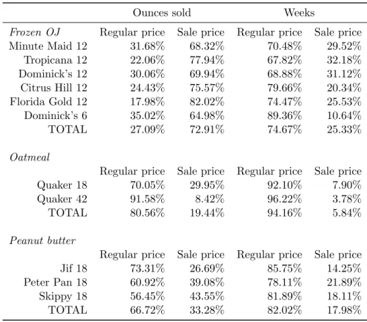
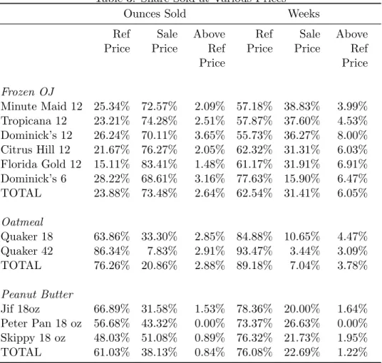
Having concluded that sales are strategically timed by the retailer, we next explore their implications for consumers. Specifically, we examine the effect of sales on prices paid by consumers and quantities purchased. Tables 2 and 3 show, for each of our UPCs, data on percent of weeks during the sam-ple and the percent of total units sold with discounted prices. Table 2 defines the sales using our variant of the Kehoe–Midrigan algorithm. Table 3 repeats the calculations when we use the EJR algorithm to select regular prices and define sales prices to be those prices which are below the reference price. It is unsurprising that quantity sold increases substantially when a prod-uct experiences a price redprod-uction. However, the combination of frequent, staggered discounts along with consumers who readily switch brands and time purchases means that a substantial fraction of all of the units sold are sold at prices below the “regular” price.12 For the two DFF categories, we find that the share of total ounces purchased on sale is approximately three times the number of product-weeks during which sales were held. Peanut butter consumers in Charlotte are somewhat less responsive to sales; for the peanut butter category we find that the share of total ounces purchased on sale is approximately twice the number of product-weeks during which sales were held. Within the peanut butter category, there is some variation across
12
The large percentages of transactions that take place at sales prices are not surprising. Kehoe and Midrigan mention this observation as one of their observations about the Dominick’s data. Bronnenberg, Kruger and Mela (2008)’s IRI data set covers 30 categories of goods at over 100 grocery chains in 50 different geographical markets. Their Table 2 shows the fraction of products that are sold on any deal and the mean percentage is 36.8%; more than 30% are sold on deal in 25 of the 30 categories they study. Griffith et al. (2009) also find that about 29.5 percent of total food expenditure from a large sample of British households is on sale items. Hence, the findings for our three categories are very typical of what happens in grocery stores.
our eight comparator cities in the measured overall responsiveness to sales. The lowest responsiveness is Knoxville, where the share of ounces sold on sale is 23 percent greater than the share of product-weeks with sales. The greatest responsiveness is our data from Hartford, where, over our seven year sample, only 7 percent of product-weeks have sales, but 57 percent of the total ounces sold are purchased at a sale price.
But there is some interesting heterogeneity in the fraction of weeks on sale and the responses. First, the six ounce store brand of orange juice goes on sale infrequently relative to the other juices—about ten percent of total weeks, yet it still garners sixty five percent of its sales in those weeks. Loosely speaking it appears that shoppers mostly prefer the larger package sizes and are quite willing to shift towards the smaller house brand when it is being discounted.13
Second, we chose to examine oatmeal because we expect it to be dis-counted less frequently than frozen OJ. That is what we find. Interestingly, we do see evidence of substantial hoarding in sales of the 18 ounce package, with quantities purchased more than tripling when it is put on discount. The purchase response by buyers of the large oatmeal packages to a discount is less pronounced. This contrast also seems reasonable given the difficulty in storing the larger package; notice also that the average price per ounce of the large package is about 25 percent cheaper than the smaller package. From Figure 9 we can see that early in the sample there are some cases where even when the smaller package is on sale, it is not cheaper on a per ounce basis than the larger package; see Griffith et al. (2009) for additional more direct evidence of the heterogeneity in households willingness to buy in bulk to save money. The percentage declines in the price when the large package is discounted are not as great as for discounts on the smaller package.
The peanut butter data illustrate that the pattern of sales and regu-lar prices can differ significantly across brands. For the Charlotte store, discounts are more frequent for Peter Pan (22 percent of weeks) versus Jif (14.4 percent of weeks). Unsurprisingly, then, a large fraction of the units of Peter Pan peanut butter are sold on sale. This raises an important fact; ignoring sales in examining pricing behavior can distort inferences not only across categories, but even across brands within the category.
Finally, notice that using our variant of the Kehoe and Midrigan algo-13The 6oz juice discounts are concentrated in the latter half of the sample. Dominick’s
appeared not to use the 6oz product as a promotional vehicle during the first half. Around this time, Dominick’s was very enthusiastic about running “fifty cent” sales promotions in which all of the items featured prominently in their sales circular were on special for fifty cents. The sale price of the 6oz juice appears to fit in with the fifty cent sale strategy.
rithm, we find fewer sales, in general, than when using the Eichenbaum, Jaimovich, and Rebelo reference price methodology. This stems mechani-cally from the fact that the methodology in EJR is not designed to measure “regular” price changes within the quarter. For example, if a price is re-duced two weeks before the end of the quarter, and the new price continues throughout the next quarter, our methodology codes that change as a shift in the regular price, not a sale. For EJR, that same price sequence is coded as a price that deviates from the reference price for two weeks, and equals a new reference price at the beginning of the next quarter.
4.3 Best Prices
To quantify the impact of strategic shopping on prices paid and facilitate comparisons of results with previous studies, we convert the weekly data into quarterly data. We calculate two useful measures of pricing. First, we calculate the “price paid” by aggregating purchases over the quarter and using transactions as the weighting mechanism, rather than time. That is, we calculate the average price actually paid by consumers for for every ounce purchased during the quarter.
One way to gauge the importance of bargain hunting is to compare the actual price paid to the best possible price that could be obtained by a consumer who is willing to undertake storage and views all brands as perfect substitutes. To compute the “best” price, we consider a hypothetical shopper in a product category who concentrates all purchases over a certain interval into whichever good is cheapest. The best price reflects the limiting case in our model, the case where every shopper is a bargain hunter and has no deterioration in demand from waiting across periods to buy.
We are forced to make an assumption about the horizon over which bargain hunters can be expected to hunt for sales and stockpile. We use the information about how frequently sales are held to infer this. Empirically, we know that some discount occurs in roughly 88% of the weeks for frozen OJ, about half of the weeks for peanut butter in our Charlotte store and about 11% of the weeks for oatmeal. Thus, we posit that the purchasing horizon is shortest for frozen OJ and longest for oatmeal. For frozen OJ we assume that optimization occurs over 3 week intervals and that the shoppers have perfect foresight about coming sales. So, for each week we compute the “best price” as equal to the lowest price (per ounce) in the category that week, the week before and the week after. Thus, we construct a best price over a three week window for every week. The average best price for the quarter is the average of the 13 weekly best prices. For oatmeal the
storability leads us to allow for a 7 week window so that the hypothetical shopper is scanning three weeks forwards and backwards at each week. We use a 5 week window for peanut butter, reflecting the fact that sales for peanut butter are more common than oatmeal but not as frequent as for orange juice. For each category, for the horizon chosen, a consumer can almost always find a sale if s/he is willing to search weekly over the horizon. We compare the actual price paid to the “best price” series as well as the two fixed weight price series discussed above. One is the fixed weight average of the reference price for each constituent UPC and the other is the fixed weight average of the list prices. The fixed weights are all computed based on the constituent product’s share of total ounces over the first quarter of our sample. The quarterly prices to which the fixed weights are applied are constructed by equal weighting the weekly prices for the UPCs in the quarter.
Figure 11 shows the resulting series for frozen OJ. The actual price paid tracks the best price remarkably well; the correlation is 0.92. Recall that in the model, if there were a constant fraction of shoppers who were loyal to one brand, then these people’s prices paid would track the list prices for that brand. If there were groups loyal to each brand plus bargain hunters, the average price paid of the loyals would equal a standard fixed weight index and the average price paid of the bargain hunters would equal the “best” price. In this case, the inactive shoppers would lead the average price paid to be a relatively constant amount above the best price. This description seems to describe well Figure 11.
Figure 12 shows the analogous data for oatmeal. As we saw in Figure 11, sales are much less common for oatmeal than the other two categories, yet the price paid still closely tracks the best price; the correlation is 0.95. This tracking indicates that shoppers are timing their purchases to take considerable advantage of the sales when they do occur.
Figure 13 shows the four series for creamy peanut butter in Charlotte. Once again the price paid mirrors the best price; the correlation is 0.81. In this case the gap between the average list price and the price paid is lower than in the other two categories. This is because there are a substantial number of consumers who choose Jif despite the fact that Peter Pan is almost always cheaper. This accounts for the earlier finding that fraction of units bought on sale is only twice the fraction of weeks where sales occur in the peanut butter category in Charlotte. In the two categories at Dominick’s, we find that purchases are more responsiveness to discounts. Turning to peanut butter in the other cities, our data suggest that the correlation between price paid and best price ranges from a low of 0.63 in Knoxville to a high of 0.93
in Houston and averages 0.82.
Recall from Table 1 that sales happen about 88% of the weeks for frozen OJ, about half the time for creamy peanut butter in Charlotte, and only about 11% of the time for oatmeal. Yet, price paid is strongly correlated with best price for all three categories. For frozen OJ and creamy peanut butter, the tracking indicates either a willingness to actively switch across brands every week or to hoard substantially every few weeks when the pre-ferred brand comes up for a sale. For oatmeal the only explanation for the tight association is inter-temporal storage, whereby people bulk up pur-chases during the sale periods.
4.4 Demand Variability
Our model posits that the high percentages of purchases on sale reflect strategic cross-product and cross-time substitution by bargain hunters. If so, then the quantities sold for an individual product and the quantities sold in a given week will fluctuate as consumers substitute across time and across products. However, this does not imply that demand is volatile, nor that consumption is volatile. Thus, we expect that the total quantity pur-chased within the product category will be more stable than the purchases of individual UPCs. Furthermore, if consumption is unaffected by sales and consumers are merely stockpiling, then the surge in quantities purchased