Risk Preferences Beyond Expected Utility Theory:
Theoretical and Experimental Approaches
Inauguraldissertation
zur Erlangung des Doktorgrades
der Wirtschaftswissenschaftlichen Fakultät
der Universität Augsburg
vorgelegt von
Diplom-Volkswirt Maximilian Rüger
Augsburg, den 28. Januar 2011
Die mündliche Prüfung fand am 17. Juni 2011 statt
Erstgutachter:
Prof. Dr. Mathias Kifmann
Zweitgutachter:
Prof. Dr. Robert Nuscheler
Theoretical and Experimental Approaches
Maximilian R¨
uger
1January 28, 2011
1University of Augsburg, Chair of Public Economics, Universit¨atsstr. 16, D-86159 Augsburg, Germany. Phone: 0049-(0)821-5984209. E-mail: [email protected].
Contents
I
Introduction
1
II
Theoretical Approaches Based on Reference Dependence
13
1 Higher-Order Risk Preferences 14
1.1 Introduction . . . 14
1.2 Theoretical Background . . . 17
1.2.1 Higher Orders . . . 17
1.2.2 Reference Dependence . . . 20
1.2.3 Higher Orders under Reference Dependence . . . 25
1.3 Results . . . 28
1.4 Implications . . . 35
1.5 Alternative Models . . . 42
1.5.1 Disappointment . . . 45
1.5.2 Regret . . . 49
1.5.3 Exogenous Reference Points . . . 54
1.6 Conclusion . . . 58
1.7 Appendix: Proofs . . . 60
2 Multi-Attribute Anticipatory Utility 74 2.1 Introduction . . . 74
2.2 Common Features of All Models . . . 79
2.4 An Alternative Model . . . 86
2.5 Functional Form of Gain-Loss Utility . . . 88
2.6 Generality of Pure Consumption Utility . . . 92
2.7 Equality of Models for Single-Attribute Utility . . . 95
2.8 Inequality of Models for Multi-Attribute Utility . . . 96
2.8.1 Substitutability of Changes . . . 97
2.8.2 Changes in Beliefs on Correlation . . . 99
2.9 Conclusion . . . 101
2.10 Appendix: Alternative Models . . . 103
2.11 Appendix: Proofs . . . 105
III
Model-Independent Experimental Approaches
112
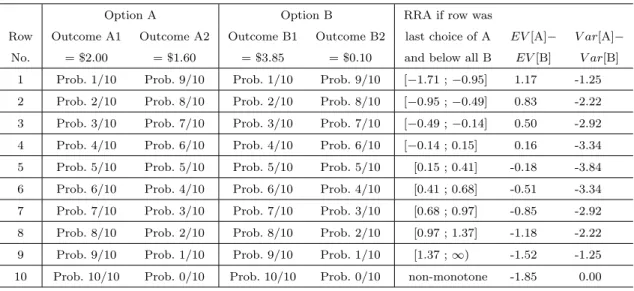
3 Intensity of Risk Aversion 113 3.1 Introduction . . . 1133.2 The Holt and Laury Method . . . 115
3.3 A Model-Independent Method . . . 117
3.4 The Experiment . . . 121
3.5 Results . . . 123
3.5.1 Directions of Risk Attitudes . . . 123
3.5.2 Intensities of Risk Attitudes . . . 124
3.5.3 Robustness . . . 132
3.6 Conclusion . . . 135
3.7 The General Model-Independent Method . . . 136
4 Measuring Higher-Order Preferences 141 4.1 Introduction . . . 141
4.2 Theoretical Prerequisites . . . 143
4.3.1 First Date . . . 148
4.3.2 Second Date . . . 149
4.4 Results . . . 155
4.4.1 Pooling Subjects . . . 155
4.4.2 Comparing Subjects . . . 157
4.4.3 Relating Risk Preferences of Different Order . . . 161
4.4.4 Comparing Domains . . . 165
4.4.5 Cumulative Prospect Theory . . . 168
4.4.6 Robustness . . . 169
4.5 Conclusion . . . 172
IV
Conclusion and Outlook
174
1.1 Second-order effects with exogenous references . . . 56
1.2 Third-order effects with exogenous references . . . 56
1.3 Fourth-order effects with exogenous references . . . 57
2.1 Second order derivatives in the continuing example . . . 82
2.2 Content of beliefs in an example with two dimensions . . . 87
3.1 The Holt and Laury method . . . 115
3.2 Our elicitation method . . . 117
3.3 Our adjusted elicitation method . . . 122
3.4 The adjusted Holt and Laury method . . . 123
3.5 Wilcoxon signed-rank tests (HLo and MRa) . . . 129
3.6 Wilcoxon signed-rank tests (HLa and MRo) . . . 129
3.7 Our generalized elicitation method . . . 137
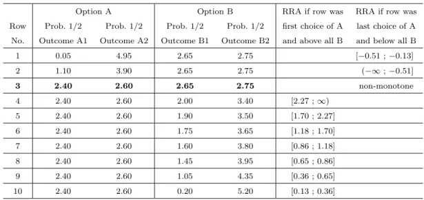
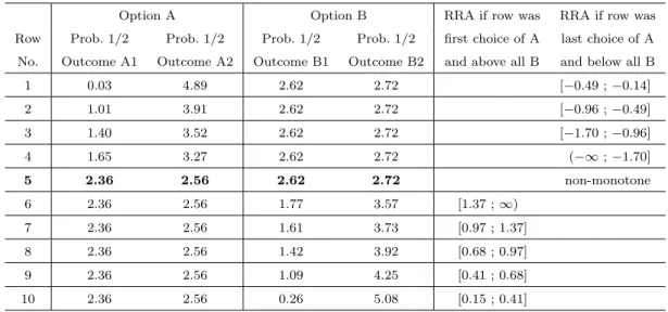
4.1 Decisions eliciting risk aversion . . . 150
4.2 Decisions eliciting prudence . . . 152
4.3 Decisions eliciting temperance . . . 154
4.4 Descriptive results pooling subjects . . . 155
4.5 Wilcoxon signed-rank tests: differences across risk preferences? . . . 165
4.6 Wilcoxon signed-rank tests: does risk aversion depend on domains? . . . 166
4.7 Wilcoxon signed-rank tests: does prudence depend on domains? . . . 166
4.8 Wilcoxon signed-rank tests: does temperance depend on domains? . . . 167
4.11 Does the elicited temperance depend on the ordering of decisions? . . . 171
List of Figures
2.1 The argument of the gain-loss function µ(·) . . . 852.2 Functional form of the gain-loss function µ(·) . . . 91
2.3 Equality of mFt,τ(p) and m(cFt,τ(p)) withK = 1 . . . 97
3.1 Cumulative distributions of RRA for all tables . . . 126
3.2 Cumulative distributions of RRA: Comparing methods . . . 127
3.3 Cumulative distributions of RRA: Comparing stakes . . . 128
4.1 Characterizing subjects: Risk aversion . . . 158
4.2 Characterizing subjects: Prudence . . . 159
4.3 Deck and Schlesinger (2010, Figure 4): Prudence . . . 159
4.4 Characterizing subjects: Temperance . . . 160
4.5 Deck and Schlesinger (2010, Figure 3): Temperance . . . 161
4.6 Relation of risk aversion and prudence . . . 162
4.7 Relation of risk aversion and temperance . . . 163
Risk preferences of economic agents are of fundamental importance for present day eco-nomic analysis. The presence of uncertainty is undeniably a key factor in shaping ecoeco-nomic behavior. The canonical model of expected utility theory (EUT) and several structural as-sumptions concerning the form of the value function have served as the working horses of theoretical and applied microeconomics for over half a century.
From a choice-theoretic perspective, the central element of EUT is that probabilities enter linear into the function determining choices. In applying EUT, it has become cus-tomary to additionally assume unifying properties concerning the value function. The value function evaluates outcomes and is multiplied with the respective probabilities to generate overall decision utility. I will give a short exemplary discussion of some of these customary assumptions on the value function.
Inside EUT, derivatives of the value function have been linked to economic behavior even before an axiomatic characterization of expected utility has been provided. A positive first derivative is equivalent to positive marginal utility. The combination of a positive first and a negative second derivative is equivalent to risk aversion. These assumptions constitute basic building blocks of every textbook on microeconomics. An important common feature of these equivalences is that explicitly or implicitly it is assumed that the sign of the derivative of a certain order is constant over the whole range of outcomes.
Assumptions concerning higher derivatives of the value function are less customary in textbooks, but have nevertheless been applied extensively in economic models. One of the economically most important forms of behavior is that of saving. From a microeconomic view, the motives to save have been identified as a desire to smooth consumption over time, and to prepare for unfavorable contingencies in the future. The latter motive is undoubtedly linked to uncertainty. If the individual wants to save more if the future is uncertain, this higher level of saving is denoted as precautionary saving. It has been clear since Leland (1968) and Sandmo (1970) that the first two derivatives of the value function cannot explain such a behavior. Instead, a positive third derivative as an additional assumption is a sufficient and necessary condition for precautionary saving to exist. Similarly, a negative fourth derivative
has been linked to risk attitudes under a stochastically independent background risk. The literature on these higher-order risk preferences in EUT models has developed substantially in the last two decades. Nevertheless, some basic puzzles concerning the empirical validity of such models remain.
Another set of assumptions concerning the value function deals with the question of how several influences of behavior interact to form the utility according to which decisions are made. In case of more than one influence on utility this is termed multi-attribute utility. The utility depends on several arguments or attributes.
A very classical example of multi-attribute utility is how levels of consumption in differ-ent future points in time shape the utility function that describes behavior in the presdiffer-ent. Expected utility theory per se does not restrict the functional form of such inter-temporal utility functions beyond the linearity in probabilities. However, it seems fair to state that the customary application in expected utility puts a lot more structure on the inter-temporal utility function. To assume a (quasi-)additive structure of inter-temporal utility has become so common that its explicit statement is often omitted.
In addition to inter-temporal aspects, multi-attribute utility has been immensely produc-tive in answering questions on how several goals at a given point in time can jointly influence the overall decision utility. In contrast to inter-temporal utility, it has been precisely the omission of an additive structure that allowed the fruitful analysis of the complex interplay between different goals. Although economists sometimes assume additive separability in or-der to obtain tractability in complicated models, it is without dispute that this comes at the cost of a lower degree of realism.
Expected utility has normatively desirable features that makes it a relatively undisputed favorite for prescriptive decision making. It ensures a high degree of consistency and ratio-nality. However, in terms of a descriptive theory that aims at describing behavior of typical economic agents, its strengths become its weaknesses. The empirical findings of systematic violations of basic axioms of expected utility by economic agents have subsequently called into question, whether reasonable predictions of behavior should be based on the hypothesis
of expected utility maximization.
There are two meaningful responses to the perception of the failure of expected utility theory as a descriptive theory. The first response is to develop detailed models of economic behavior that extend expected utility. The second response is the development of methods that do not require the assumption of a specific model of behavior.
The new alternative theoretical models should incorporate insights on what determines economic behavior from empirical studies, experimental evidence, psychology and common sense. They should be built subsequently, based on the work of other researchers and they should try to further improve these models. Part II of this thesis aims to contribute to this endeavor. I briefly outline the theoretical modifications of expected utility that have advanced the search for an improved model.
A radical approach would be to abandon the assumption that behavior can be described by the outcome of an optimization process. In place of the hypothesis of optimization steps the assumption that individuals follow a set of heuristics. While the psychological evidence for simple heuristics may be favorable in many situations, this approach comes at a huge cost. If one allows for many different simple and situation-specific heuristics, one leaves behind the ambition to find a relatively universal explanation of human behavior. The question which heuristic should be applied in which situation becomes tedious and to a certain degree arbitrary. Also, out of context predictions seem unobtainable. If a heuristic is used to describe behavior in a well-observable setting and this explanation is very context-specific, difficulties arise in extending this theory to other contexts. However, these out of sample predictions are the ultimate goal of any theory.
A less radical deviation from the standard model is to account for the fact that individuals might act altogether in accordance with the optimization of a objection function, but in doing so make systematic mistakes. These biases are often occurring in well-defined classes of decision problems. Examples are inter-temporal or inter-contextual inconsistencies. These can often be described as self-control problems. Here, the individual might want to commit to an action that she anticipates she will have difficulties in following through in other
circumstances.
A fruitful extension of the expected utility model has been to maintain the formal struc-ture, but to define the exact content of the argument of the value function more carefully. In textbook models, the argument of the value function is predominantly stated as wealth, disposable income, or the consumption of narrowly defined goods and services. However, by incorporating a wider range of objectives into the value function, the basic structure of EUT can be maintained and the descriptive accuracy highly enhanced. Examples for helpful enhancements are the incorporation of emotions, aspirations, habits, and feelings of fairness, equity and justice into the value function. An extension used in in chapter 2 of this thesis is the notion that the expectation of future consumption and changes in this expectation can be carriers of utility in the present. I will refer to such models as anticipatory utility.
The extensions of EUT discussed so far have contributed to a certain degree in improving the standard model. However, the vast majority of extensions have taken the approach to make less substantial changes. Instead, they have investigated which small departures in the structural assumptions lead to better predictions. These changes in the structure can be distinguished according to whether the focus is on the influence of probabilities or on the shape of the value function.
The predominant focus of theoretical economic research on decision making in the 1980s and 1990s that was seeking to extend EUT attempted to include nonlinear influences of prob-abilities. These extensions tried to capture the perception that individuals have difficulties in assessing probabilities which are very small. This was achieved by applying a probability weighting function to every probability before aggregating over the states of nature. Early models based on a longer tradition in psychology took a dual approach were each probability is transformed by a function independently of the corresponding outcome. It was soon noted (e.g. by Fishburn, 1978) that this leads to violations of stochastic dominance, which discred-ited the model. A solution was found by Quiggin (1982), who introduced rank-dependent expected utility which allows a non-linear influence of probabilities without violating stochas-tic dominance. The central questions in this field seem to be solved. Therefore, recent studies
focus on the precise parametrical characterization of the probability weighting function. The remaining obstacles concerning probabilities are likely to stem from the fact that individuals fail to execute Bayesian updating, or lack the capability to form subjective probabilities in the first place.
Only in recent years the importance of the shape of the value function was recognized by a broad group of researchers. Of special importance to the shape of the value function is the concept of a reference point. The reference point is the notion that an important aspect leading to a decision is the comparison of the alternatives in relation to a mental anchor. If a potential outcome exceeds this reference point it is perceived as a gain, if it falls below the reference point it induces sentiments of loss.
The influence of reference points is well-established in psychology. It originates from the field of psychophysics, which can be defined as the quantitative analysis of the relationship between physical stimuli and the resulting sensations. A classical example is an experiment where subjects first place one hand in cold and one hand in hot water. After some time, both hands are placed into water of intermediate temperature. Although both hands are now exposed to an identical temperature, the subject thinks that the hand which was placed in the hot water before, is now exposed to a lower temperature, and vice versa. The reason is that the reference temperature is different for both hands, and the present temperature is partly evaluated by a comparison to this reference temperature.
In the economics literature, the role of the stimuli is played by the extent that wants are met. Early economics literature on reference points were Markowitz (1952) and Kahneman and Tversky’s (1979) prospect theory. In these early models the reference point is assumed to be a real-valued variable. The influence of such a reference point on the shape of the value function then can be twofold.
First, the reference point determines the reflection point of the value function. The reflection point captures the idea that the second derivative of the value function does not need to have a constant sign. In the model by Kahneman and Tversky (1979), the value
function is concave above the reference point and convex below the reference point.1 This
would capture the idea that individuals are risk-seeking in losses and risk-averse in gains. The empirical assessment of whether individuals are really risk-seeking in losses is still mixed and seems to depend on the context. The assumption of a reflection point itself is compatible with arbitrary levels of differentiability of the value function.
Second, the reference point also determines loss aversion. If the value function is rep-resented by a graph, loss aversion is a concave kink at the reference point. By allowing for a kink, one abandons the property of differentiability over the whole range of the value function. Often it is assumed that the value function is differentiable at all other levels than the reference point. Therefore, calculus can still be used when analyzing behavior concern-ing situations with outcomes entirely strictly above (or entirely strictly below) the reference point.
The literature on reference points has developed substantially in recent years. Two major developments can be identified. First, the reference point is no longer generally assumed to be a single point. In recent models (Sugden 2003; Delqui´e and Cillo, 2006; K˝oszegi and Rabin, 2006, 2007, 2009) the reference point is a whole distribution potential outcomes are compared to. This captures the idea that individuals can make multiple comparisons in order to evaluate the desirability of an outcome. Second, the reference point was endogenized by K˝oszegi and Rabin (2006, 2007, 2009). This is of high importance since an arbitrary exogenous reference point was one of the main obstacles raised by critics of such models. K˝oszegi and Rabin derive how recent expectations can shape the reference point.
A more detailed overview over the recent development on reference points, its applications and empirical assessment is provided in chapter 1 of part II of this thesis. Nevertheless, it seems appropriate to stress that existing models of reference-dependent preferences focused almost entirely on risk aversion and behavior that follows directly from risk aversion. Some of
1In the model of Markowitz (1952) the reverse is true for small deviations from the reference point.
However, he assumes as well that for larger deviations from the reference point the value function becomes locally concave in gains and locally convex in losses. This would indicate the existence of three reflection points. Also, the classical value function of Friedman and Savage (1948) exhibits two reflection points, although they do not refer to the concept of a reference point.
the results in K˝oszegi and Rabin (2007) can be interpreted as statements on behavior under background risk and K˝oszegi and Rabin (2009) include a short discussion of precautionary behavior. However, no systematic treatment of higher-order risk preferences was attempted so far. The existing results were derived only in narrowly defined models. I therefore consider it worthwhile to fill this gap.
Eeckhoudt and Schlesinger (2006) defined higher-order risk preferences in terms of simple gamble definitions. Chapter 1 in part II of this thesis employs these model-independent definitions in a systematic way to study higher-order risk preferences in models of reference-dependent preferences. This theoretical application is joint work with Johannes Maier from the University of Munich. We find that in the framework of K˝oszegi and Rabin (2006, 2007), individuals exhibit even- but never odd-order risk attitudes. We further use these results to explain empirical patterns of seemingly sub-optimal behavior concerning precautionary saving and insurance demand, that have been described as puzzles in the literature.2 In
order to show that our results only obtain when expectations shape the reference point, we also analyze alternative models and find that they deliver other or even opposite patterns of higher-order risk preferences.
K˝oszegi and Rabin (2009) extend their framework of endogenously defined reference-dependent preferences to the realm of anticipatory utility. They also provide a multi-attribute formulation of their model. However, in chapter 2 of part II of this thesis I will argue that the precise form of the model proposed suppresses the major advantages of multi-attribute utility. K˝oszegi and Rabin’s (2009) definition of reference-dependence restricts utility to be additively separable.
In chapter 2, I will outline an alternative formulation that follows the same basic intuitions as K˝oszegi and Rabin (2009), but which is also applicable if utility is not additively separable in arguments. It is shown that for utility functions with a single dimension, the two models coincide. However, if the utility function has several dimensions, the two models differ,
2See, for instance, the overview article by Caroll and Kimball (2008) on empirical evidence on
precau-tionary saving falling short of optimal levels in traditional models. See Gollier (2003) on an apparent excess of insurance demand in the presence of buffer stock saving.
even if the utility function is additive separable. Therefore, although my model has a larger domain of applicability, it is not a mere generalization of the previous model. Two examples are discussed to show that this difference with additive-separable utility applies to practically relevant situations. First, only in my model, simultaneous changes in different dimensions of consumption that would not result in an overall effect on pure consumption utility, do not have an effect on reference-dependent anticipatory utility. Second, an update in beliefs over the correlation of risks affecting different dimensions of pure consumption utility, generates a change in decision utility only in my model.
The in-depth engagement in the advancement of theoretical economic models raises a general methodological question regarding the final goal of this task. It is closely related to the fraction of individuals one seeks to model by a given model. Are we searching for a unifying theory to describe the vast majority of individuals in any setting? Or would we be satisfied with a tractable set of theories where each theory would describe a subset of individuals? For example, Harrison, Humphrey and Verschoor (2010) find in a series of experiments that about half of their subjects can be described relatively accurately by EUT, while the other half generally acts in accordance with prospect theory (PT).
If heterogeneity of individuals basic preference structure is accepted, we face the serious problem of how to construct methods of preference measurement that can be applied to the whole set of individuals. Statements, such as that one subject is more risk averse than another one, are difficult, if the applied method relies on assumptions specific to EUT or PT. General propositions on behavior, especially comparing individuals, become hard to obtain. Even if we do not accept that individuals may be fundamentally different in their basic preference structure, we might face a similar problem. The constant advancement of the-oretical models can make a method of measurement based on a specific formulation of a theory rapidly out-dated. Empirical assessments of preferences building on different specific models may be incomparable. Also, the challenge arises of how to deal with uncertainty of the modeler on which is the right model. Should he conduct a multitude of preference elicitations, each tailored to a different model?
A way out of both of these dilemmas is the development of model-independent tools. By these, I refer to methods that do not require the assumption of a specific model of behavior. Instead, they apply to a wide range of models that have been proposed. This does not mean that we make no assumptions at all. We always need some assumptions, otherwise we are not in the position to measure anything. However, the required assumptions are of a general nature and are shared by a wide range of models. If the method is based only on these general assumption, its results can be informatively applied in all these models. Part III of this thesis, which is based on joint work with Johannes Maier, contributes to this literature in the form of two experimental studies.
In the analysis of risk preferences, the most fundamental model-independent measure concerns risk aversion. A theoretical concept of risk aversion that does not rely on a specific model would be, for example, whether an individual prefers a sure payment of the expected value of a lottery over the lottery itself. There is a vast amount of experimental work that can be interpreted in this sense. Therefore, we consider the issues as settled with respect to this qualitative direction of risk aversion.
However, the measurement of the intensities of risk aversion is model-dependent for the prevailing experimental methods. This is despite the fact that there also exist well established model-independent definitions of an increase in risk.3 Building on these, we can define an individual as more risk averse than another one if she is ready to accept more increases in risk as a trade-off to a certain reward.4 This establishes a definition of being more risk averse
that can be applied in any commonly proposed model. In chapter 3 in part III of this thesis I discuss our model-independent methodology to measure risk aversion in the laboratory. We implemented the method in an experiment jointly with the risk aversion elicitation method of Holt and Laury (2002). Nowadays, this is the risk aversion elicitation method most widely used in economic experiments, although it is based on specific assumptions of EUT. By implementing both methods simultaneously in our experiment, we can compare
3The most prominent definition of increasing risk is the concept of mean-preserving spreads by Rothschild
and Stiglitz (1971) which will also be applied by us.
the results of both methods in a within-subject analysis. We show that the differences in the two methods are not only of a methodological nature, but also that they yield substantially different results.
Although the experimental evidence on risk aversion is vast, on higher-order risk prefer-ences it is quite scarce. The few experimental studies that exist are very recent. Therefore, there are no established experimental methods to measure higher-order risk preferences. We provide a contribution to this emerging field of study that I discuss in chapter 4 in part III of this thesis. The experimental studies can be based on the model-independent definitions of higher-order risk preferences by Eeckhoudt and Schlesinger (2006). Therefore, they meet the criterion of model-independent measurement outlined above.
Deck and Schlesinger (2010) is so far the only published experiment on higher-order risk preferences. They find evidence for prudence (downside risk aversion), but at the same time against temperance (outer risk aversion) in their subject pool. Within EUT the com-monly assumed parametric value functions (such as those of constant absolute or relative risk aversion) cannot exhibit this combination. In contrast, such a combination is compatible with proposed parameterizations of prospect theory. Deck and Schlesinger (2010) therefore interpret their findings as support of prospect theory.
A key feature of many non-EUT models including prospect theory is the distinction between gains and losses. In experiments, gains and losses are most often only differentiated by the framing of subjects decisions. This is mainly due to institutional constraints that prevent researchers to inflict real monetary losses on subjects. However, framing effects are elusive and considered by some economic methodologists as non-informative for economic questions. Therefore, we specifically designed our experiment to induce real monetary losses on subjects. To do so, we implemented a design that separates the experiment over two dates, several weeks apart. At the second date we were allowed to inflict real losses on the subjects, confined by their earnings of the first date.
We found that subjects generally are prudent and temperate. This general pattern holds for decisions in gains as well as in losses. Our findings of temperance are in contrast to the
results of Deck and Schlesinger (2010) and therefore lead to diverging conclusions. Also, in our experiment, risk preferences of different orders are highly correlated.
In part IV of this thesis I provide a brief conclusion of the presented results. Also, an outlook is given on how the taken route of research can be traveled further in the direction of more general concepts of uncertainty than risk.
Theoretical Approaches Based on
Reference Dependence
Chapter 1
Higher-Order Risk Preferences
∗
1.1
Introduction
While the well-known second-order effect of risk aversion describes a preference for less uncertainty, higher-order risk preferences characterize how this preference changes under dif-ferent circumstances. For instance, the third-order effect of prudence plays an important role for changes in risk aversion due to variations in wealth, and the fourth-order effect of temper-ance is crucial for changes in risk aversion in the face of a background risk. The theoretical literature on these higher orders is well-developed (building on Kimball, 1990, 1992) since the importance of prudence for phenomena like precautionary saving was recognized early (Leland, 1968). While numerous empirical studies find supportive evidence for the presence of precautionary saving, they also show that it is usually too low to be consistent with those theoretical models and common assumptions about risk aversion.1 Also, contrary to
obser-vation, optimal precautionary saving should theoretically lead to substantial crowding out of insurance demand (Gollier, 2003).
∗This chapter is based on joint work with Johannes Maier. Both authors contributed equally to this
work.
1For instance, the test of Dynan (1993, p1104) “. . . yields a fairly precise estimate of a small precautionary
motive; in fact, the estimate is too small to be consistent with widely accepted beliefs about risk aversion.” In an overview article Carroll and Kimball (2008, pp583-584) conclude that “. . . estimates of relative risk aversion imply precautionary saving motives much stronger than those that have been used empirically to match observed wealth holdings. This discrepancy remains unresolved.”
Until now, theoretical models analyzing higher-order risk preferences were constrained to the framework of expected utility theory (EUT) in which they correspond to the derivatives of the utility function. In contrast, in order to resolve various empirical puzzles concerning second-order risk preferences, a prominent strand of literature (starting with Kahneman and Tversky, 1979) evolved that stresses the dependence of preferences on a reference point. The latest advancement in this literature was made by K˝oszegi and Rabin (2006, 2007) who en-dogenize recent expectations as the reference point. We analyze higher-order risk preferences within their model of reference-dependent preferences. We further show that our results can explain seemingly sub-optimal levels of precautionary saving and insurance demand. As a robustness analysis, it is also shown that alternative models, like disappointment, regret, or exogenous reference points yield different results and cannot resolve these empirical puzzles concerning higher-order risk preferences.
Section 1.2 presents the two concepts that are merged in this chapter and gives the the-oretical background that is needed in order to understand how we derive our results. In section 1.2.1 we follow Eeckhoudt and Schlesinger (2006) and define lotteries that represent higher-order risk preferences independently of a specific model. It is their gamble represen-tation that allows us to analyze higher orders in the model of K˝oszegi and Rabin (2007) which is presented in section 1.2.2. In order to make our results comprehensible as well as comparable to each other, we transform choices such that they reflect preference relations as if the reference point was zero. This method of transformation is explained in section 1.2.3. Our results are presented in section 1.3. We show that individuals with expectation-based reference-dependent preferences are neither prudent nor imprudent while second- and fourth-order effects are still present. More specifically, using common functional forms of gain-loss utility we show that individuals are risk-averse and intemperate, but they are indifferent toward the third order independent of the functional form of gain-loss utility. While risk aversion is also predicted by classical EUT models, third- and fourth-order behavior differs substantially under reference dependence. We generalize these results for risk preferences of arbitrary order n and show that those of odd orders (except order one) are absent while
those of even orders are still present. The intuition for this result is based on the fact that odd-order risk preferences can always be thought of as a decision on the location of risk(s), whereas even-order risk preferences are concerned with the aggregation of risk(s). Due to the anticipation of choices, the location does not matter for sensations of gains and losses.
In section 1.4 some of the possible economic implications of our results are discussed. In general our results show that it may be highly problematic to derive optimal behavior that rests on preferences of higher orders from measures of risk aversion. With reference-dependent preferences combinations of certain risk attitudes are possible that cannot be consistently derived within EUT. More specifically, we show that empirical findings on seem-ingly sub-optimal amounts of precautionary saving under classical EUT can be attributed to the optimal behavior of individuals with expectation-based reference-dependent preferences. The reason is that reference dependence contributes positively to risk aversion, but leaves prudence unaffected. Within classical EUT models optimal precautionary saving is directly derived from measures of risk aversion. However, if individuals have reference-dependent preferences instead, measured risk aversion will indeed be higher but not the optimal amount of precautionary saving. Also, the theoretically puzzling existence of costly insurance when capital markets are well developed and individuals can accumulate buffer-stock wealth is less surprising for such individuals. Under reference dependence second-order effects become relatively more important than third-order effects.
In section 1.5 we consider several other behavioral models in order to show that the same results do not obtain under alternative specifications of the reference point. Section 1.5.1 considers disappointment models where the reference point is the expectational mean of the chosen alternative (Bell, 1985; Loomes and Sugden, 1986). Here, we do not observe the absence of odd-order risk preferences while even-order risk preferences are similar to those of expectation-based reference dependence. In recent empirical work it has been difficult to distinguish between these two models of reference dependence. Our third-order result therefore suggests a new way how to differentiate between expectation-based reference de-pendence and models of disappointment. In section 1.5.2 we analyze higher orders in models
of regret (Bell, 1982, 1983; Loomes and Sugden, 1982) where the reference point is the alter-native that was not chosen. It is shown that decisions taken to avoid regret are unaffected by even-order effects, but odd-order effects still exist. This suggests that regret influences higher-order risk preferences in the opposite way as expectation-based reference dependence. Risk preferences of any order (except order one) differ between these two models, but regret induces similar odd-order risk preferences as disappointment models. Models with reference points shaped by expectations and regret are usually analyzed separately rather than jointly in a unified framework. However, our analysis shows the close relationship they share. Risk preferences of a particular order are only affected by either expectations or regret as the ref-erence point, but never by both. Lastly, we analyze exogenous refref-erence points, such as the status quo, in section 1.5.3. Here, results vary with the various reference points considered and attitudes concerning gains and losses. However, just as in the case of disappointment and regret, exogenous reference point do not yield the same results as expectation-based reference dependence on higher-order risk preferences. Our robustness analysis of section 1.5 therefore shows that alternative specifications of the reference point imply different results and cannot explain empirical puzzles that have been found with respect to higher orders.
Section 1.6 is devoted to the conclusion where we summarize our results and discuss further extensions. All proofs appear in the appendix of section 1.7.
1.2
Theoretical Background
1.2.1
Higher Orders
Within EUT it has long been recognized that risk preferences are not exhaustively de-scribed via the concept of risk aversion alone. Already Leland (1968) and Sandmo (1970) identified the importance of a positive third derivative of the utility function for motives of precautionary saving. Since Kimball (1990) the feature of preferences that is necessary
and sufficient for such precautionary behavior is termed prudence.2 An equivalent concept
to prudence, termed downside risk aversion, was established by Menezes, Geiss and Tressler (1980). It describes an aversion to mean-variance preserving transformations that shift risk from the right to the left of a wealth distribution. Afterward, an extensive literature de-veloped that discussed also higher derivatives of utility functions and their implications for economically important decisions under uncertainty. For instance, negative fourth deriva-tives of the utility function were shown to be crucial for risk aversion to increase with the existence of a zero-mean background risk (see Gollier and Pratt, 1996; or Eeckhoudt, Gollier and Schlesinger, 1996). This fourth-order property of the utility function was termed tem-perance by Kimball (1992) and outer risk aversion by Menezes and Wang (2005). Eeckhoudt and Schlesinger (2008) show that temperance is necessary and sufficient for precautionary saving to increase as thedownside risk of future income rises.
Outside standard EUT, preferences of higher orders have not been considered explicitly in the literature yet. Building on the concept ofnth-degree risk by Ekern (1980), Eeckhoudt
and Schlesinger (2006), however, provided definitions of all higher-order effects in terms of preferences over simple lotteries.3 This representation is quite general since it is independent
of a specific model. The authors showed that when applied in an EUT framework their definitions correspond to the common definitions in terms of derivatives used so far. Because we are interested in higher-order risk preferences under reference dependence, we employ these gamble definitions in our analysis.
Denote initial wealth by y∈R.4 Letk ∈R be a sure reduction in wealth with k >0. ˜εi
are symmetric random variables which are non-degenerate, independent of all other random
2Despite being not necessaryand sufficient, prudence has also been shown to play an important role in
other economic applications, like for instance rent-seeking games (Treich, 2010), auctions (Es˝o and White, 2004), bargaining (White, 2008), principal-agent monitoring (Fagart and Sinclair-Desagn´e, 2007), global com-mons problems (Bramoull´e and Treich, 2009), inventory management (Eeckhoudt, Gollier and Schlesinger, 1995), or optimal prevention (Eeckhoudt and Gollier, 2005; or Courbage and Rey, 2006). It has also been used in a more normative context to derive an optimal ecological discount rate (Gollier, 2010) or to justify the so-called precautionary principle (Gollier, Jullien and Treich, 2000; and Gollier and Treich, 2003).
3These lotteries have also been used in recent experiments to investigate higher-order risk preferences
empirically (see Deck and Schlesinger, 2010; Ebert and Wiesen, 2010; or chapter 4 of this thesis.
variables that affect wealth, and have E[˜εi] = 0.5 Now, we define the following standard
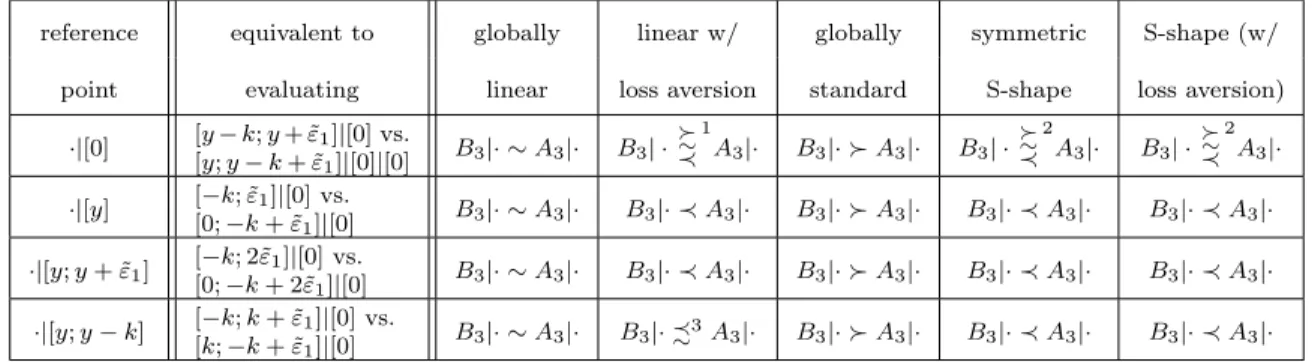
gambles, where each element denotes an outcome and each outcome of a specific gamble is realized with equal probability.6 Such defined outcomes can be either deterministic or stochastic themselves. B1 B2 B3 B4 Bn ≡ ≡ ≡ = ≡ = ≡ [y] [y] [y−k;y+ ˜ε1] [A1;B1+ ˜ε1] [y+ ˜ε1;y+ ˜ε2] [A2;B2+ ˜ε2] [An−2;Bn−2+ ˜εint(n 2)] A1 A2 A3 A4 An ≡ ≡ ≡ = ≡ = ≡ [y−k] [y+ ˜ε1] [y;y−k+ ˜ε1] [B1;A1 + ˜ε1] [y;y+ ˜ε1+ ˜ε2] [B2;A2 + ˜ε2] [Bn−2;An−2+ ˜εint(n 2)].
Intuitively, B1 vs. A1 is equivalent to the question whether more is preferred to less. B2
vs. A2 is the comparison between a certain level of wealth and a risky alternative with
an identical mean. B3 vs. A3 is equivalent to the question whether one prefers to add an
unavoidable random variable to the higher or lower outcome. It is also equivalent to the question whether one prefers to accept a sure reduction in wealth in the certain or uncertain state. B4 vs.A4 can be seen as the question whether one prefers to aggregate or disaggregate
two independent random variables.
Following Eeckhoudt and Schlesinger (2006), preferences are then
monotone risk-averse prudent temperate ⇔ ⇔ ⇔ ⇔ B1 %A1 B2 %A2 B3 %A3 B4 %A4 ∀y, k ∀y,ε˜1 ∀y,ε˜1, k ∀y,ε˜1,ε˜2 (⇔u0(x)≥0 in EUT models) (⇔u00(x)≤0 in EUT models) (⇔u000(x)≥0 in EUT models) (⇔u0000(x)≤0 in EUT models)
5Except the assumption of symmetry, all ˜ε
iare identically defined in Eeckhoudt and Schlesinger (2006).
or, more generally
risk apportioning of order n ⇔ Bn%An ∀y,ε˜1, . . . ,ε˜int(n
2), k
⇔un(x)≤(≥) 0 if n2 ∈(∈/)N in EUT models
whereun(·) denotes the nth derivative of u(·). Note that all commonly used utility functions
in EUT, like for instance those exhibiting constant relative or absolute risk aversion, have derivatives that alternate in signs withu0(·) being positive (see Brockett and Golden, 1987), a property termed mixed risk aversion by Caball´e and Pomansky (1996).
1.2.2
Reference Dependence
Reference-dependent preferences were established in economics via Kahneman and Tver-sky’s (1979) prospect theory. It introduced four novel aspects: reference dependence, loss aversion, diminishing sensitivity concerning gains and losses and non-linear probability weight-ing. Our main focus is on the first feature. Some results will be completely independent of whether the second and third features are present while other results will vary with their existence. The fourth feature of probability weighting will be absent from the whole analysis. In this respect we follow the models we discuss in this chapter.
Focusing on reference dependence immediately leads to the question of what the reference point is. In the traditional literature on prospect theory the reference point is a real numbered variable that is completely exogenous. It is a simple point which every potential outcome is compared to, and it is not influenced by the decision-maker in any way. Often, the status quo was advocated as a candidate for this reference point (e.g. Kahneman and Tversky, 1979; or Tversky and Kahneman, 1991). However, even this early literature noted that this might not be the relevant comparison in many important situations. “For example, an unexpected tax withdrawal from a monthly pay check is experienced as a loss, not as a reduced gain.” (Kahneman and Tversky, 1979, p286). Later, considerations that expectations may play a role were explicitly included into formal analysis (see Bell, 1985; Loomes and Sugden, 1986;
Sugden, 2003; Delqui´e and Cillo, 2006; and K˝oszegi and Rabin, 2006, 2007, 2009).
In early models of disappointment (see Bell, 1985; and Loomes and Sugden, 1986) indi-viduals compare potential outcomes to the mean of the choice. Every option that can be chosen has therefore its specific reference point which is thus endogenous. An advancement of disappointment models has been proposed by K˝oszegi and Rabin (2006, 2007). Here, the reference point is not simply the mean but rather the full distribution of outcomes resulting from the chosen alternative. We refer to such reference points as expectational references. This specification is motivated by the observation that individuals can make multiple comparisons to evaluate an outcome. It also accounts for the fact that individuals realize uncertainties and incorporate them into their reference point.
Expectational references have since been applied in order to explain various important phenomena. For instance, Heidhues and K˝oszegi (2008) use them in a model of price com-petition to explain sticky prices. Herweg (2010) shows that the flat-rate bias when choosing optimal tariffs can be explained when consumers have expectational references. Heidhues and K˝oszegi (2010) use expectational references in order to explain why “sale” prices in ad-dition to regular prices only exist in certain environments. Herweg, M¨uller and Weinschenk (2010) analyze a moral hazard setting with expectational references in order to explain bi-nary payment schemes. Closely related, Macera (2010) shows in a two-period model that contracts deferring all present incentives into future payments, like e.g. yearly productiv-ity bonuses combined with a present fixed wage, are optimal with expectational references. Lange and Ratan (2010) study bidding behavior of agents with expectational references in different auction formats and explain why in laboratory experiments but not necessarily in the field overbidding should be observed.
Empirical work also points toward expectations as the relevant reference point. Meng (2009) uses expectations as the reference point in order to explain the disposition effect, i.e. the observation that stock market investors tend to keep their loosing assets for too long and sell their winning ones too soon, and further finds expectations as best estimate of investors’ reference point from individual trading data. Card and Dahl (forthcoming) show that the
rate of family violence when the local professional football team loses depends on the extent to which losing the game was expected. Mas (2006) shows that the larger the difference is between requested (by the union) and received wages the more police performance declines. Pope and Schweitzer (forthcoming) show that expectation-based loss aversion is present among professional golfers suggesting that it is a bias which survives experience, competition and large stakes. Post et al. (2008) analyze game show data and find that behavior of contestants is consistent with reference points shaped by expectations. Crawford and Meng (forthcoming) (building upon previous work by Camerer et al. 1997; and Farber, 2005, 2008) propose and estimate a labor supply model of New York City cabdrivers with reference-dependent preferences where income- as well as working hour-targets are both determined by rational expectations. Using new data of New York City cabdrivers and using a natural experiment Doran (2009) finds that a permanent wage increase causes hours worked to remain constant, a finding consistent with expectations as the reference point.
Labor supply decisions have also been tested in a laboratory experiment by Abeler et al. (forthcoming). They manipulate subjects’ rational expectations and find that effort provi-sion is affected in the way predicted by expectation-based reference-dependent preferences. Ericson and Fuster (2010) show in an exchange and in a valuation experiment that the ref-erence point is determined by expectations rather than by the status quo and discuss why some researchers have not found endowment effects in different settings. Knetsch and Wong (2009) also conduct exchange experiments and suggest that expectations shape the reference point. A recent experiment by Gill and Prowse (forthcoming) finds that expectations are the relevant reference point when subjects compete in a real effort tournament. Finally, Loomes and Sugden (1987), Choi et al. (2007), or Hack and Lammers (2009) find supportive evidence for expectations as the reference point in risky choice experiments.
All the above mentioned literature is concerned with first- or second-order effects of reference-dependent preferences. In this chapter we are rather interested in higher-order effects. To our knowledge there has been no attempt to consider higher orders under reference
dependence. We follow K˝oszegi and Rabin (2007) and define overall decision utilityV(·) as V(F|G) = M(F) +U(F|G) = Z m(x)dF(x) + Z Z u(x|r)dG(r)dF(x). (1.1)
The outcome x ∈ R and the reference point r ∈ R are independently drawn from the
probability distributions F and G, respectively. Pure consumption utility depending solely on the outcome x is denoted by m(x) and thus the expected pure consumption utility is
M(F) = R m(x)dF(x). The function
u(x|r) =u(m(x)−m(r))
captures sentiments of gains and losses that occur if the outcome x is realized and the reference point was r. The expected level of gain-loss utility is denoted by U(F|G) =
RR
u(x|r)dG(r)dF(x). The assumption of independently distributed x and r captures the
notion that the evaluation of all possible wealth outcomes is based on comparing each of them to all possibilities in the support of the reference lottery. What we refer to as expectational references (K˝oszegi and Rabin, 2006, 2007, 2009) equates the reference and the outcome distribution and thereforeG=F.7
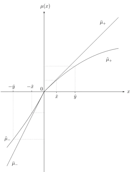
Some of our results in the following section hold independently of the functional form of gain-loss utility u(·). The remaining results depend on its specific shape. For the latter cases we will consider u functions that are usually proposed in the literature. This includes standard (weakly) concave as well as loss-averse S-shapedufunctions. S-shaped ufunctions are defined as being (weakly) concave in gains and (weakly) convex in losses (i.e. u00(τ) ≤
0 ∀τ >0 and u00(τ) ≥0 ∀τ <0). Following K¨obberling and Wakker (2005) we refer to loss aversion as a kink at the reference point zero (i.e. limτ→0u
0(−|τ|)
u0(|τ|) ≡λ >1). Furthermore, when
S-shaped utility is assumed we refer to loss-averse u functions as the standard case where
7K˝oszegi and Rabin (2006, 2007, 2009) further develop an equilibrium concept that restricts which choices
utility is diminishing faster or equally in gains than in losses (i.e.u00(τ)≤ −u00(−τ)∀τ > 0). This includes the case whereu(·) is piecewise linear with loss aversion. Often results differ for strict formulations of the functional characteristics above and the limiting cases. A limiting case of S-shaped u functions without loss aversion are symmetric S-shaped u functions. A linear u(·) is a limiting case of both weakly concave and S-shaped functions without loss aversion. Both limiting cases have in common that they are (two-fold rotational) symmetric around the reference point. This property is crucial in explaining why their results differ compared to their strict (and asymmetric) counterparts.8 Note that both strictly concave
and loss-averse S-shaped ufunctions share the common feature that losses loom larger than corresponding gains (i.e. u0(τ) < u0(−τ) ∀τ > 0).9 Throughout it is assumed that u(τ) is
strictly increasing, continuous and sufficiently often differentiable for allτ (∀τ 6= 0 if λ >1), and that u(0) = 0.
While we consider various general functional forms of u(·), we again follow K˝oszegi and Rabin (2007) in that we restrict m(·) to be linear (i.e. m0(·)> 0, m00(·) = 0).10 The reason
for this assumption is twofold. First, in models wherem(·) is assumed to be concave instead usually strong restrictions on the functional form of u(·) are needed to keep the model tractable.11 Since we are interested in the effect of reference dependence on higher-order risk 8A loss-averse S-shapedufunction is the typical assumption in the literature on reference dependence.
The reason why we additionally discuss concave as well as (two-fold rotational) symmetricufunctions is the following. In section 1.5 we consider alternative models, like disappointment or regret theory, in order to show that the results on expectational references cannot be derived using such alternative models. These alternative models can also be captured by (1.1) but with a different specification concerning the reference point. A common assumption in the regret literature is a concave u function. In their disappointment theories, Loomes and Sugden (1986) assume aufunction that is convex in gains and concave in losses but has the property of being (two-fold rotational) symmetric, while Bell (1985) assumes a piecewise linearu(·). Since there exists no a priori reason to assume that a specific functional form is limited to a specific reference scenario we rather consider all possibilities throughout.
9While evidence for this feature in the literature on reference dependence is vast, for evidence that regret
looms larger than rejoicing, see e.g. Inman, Dyer and Jia (1997) and Camille et al. (2004).
10With the exception of their proposition 9, this assumption is made throughout by K˝oszegi and Rabin
(2007) and for some results in K˝oszegi and Rabin (2006). Other more applied models in the literature impose this assumption as well (see e.g. Heidhues and K˝oszegi, 2010; Lange and Ratan, 2010; Meng, 2009; or Gill and Prowse, forthcoming). In the context of regret, Bleichrodt, Cillo and Diecidue (2010) show in an experiment thatm(·) isnot significantly different from linear. In the disappointment models of Bell (1985) and Loomes and Sugden (1986)m(·) is assumed to be linear as well.
11These models restrict attention to piecewise linear gain-loss utility (see Heidhues and K˝oszegi, 2008,
2010; Crawford and Meng, forthcoming; Meng, 2009; Herweg, M¨uller and Weinschenk, 2010; Herweg, 2010; Lange and Ratan, 2010; Macera, 2010; and some results in K˝oszegi and Rabin, 2006, 2007).
attitudes, we rather consider different functional forms that directly affect gain-loss utility u(·). Second and more importantly, higher orders are already well analyzed within classical EUT models. Assuming a concave m function would simply reintroduce higher-order effects of EUT into the gain-loss function and would therefore dilute the pure effect of reference dependence on higher-order risk attitudes.12 Moreover, reference dependence is especially
considered as important in situations where classical consumption utility is almost linear. In order to generate reasonable risk taking behavior, Rabin (2000) shows that consumption utility is compatible with risk neutrality for amounts as high as a monthly salary.
1.2.3
Higher Orders under Reference Dependence
For notational convenience we will use F|G % F0|G0 interchangeably to V(F|G) ≥
V(F0|G0) throughout the chapter. Since we are interested in higher-order risk preferences under reference dependence, we apply the gamble definitions of section 1.2.1 to the outlined model (1.1) in the following way.
Definition 1 A reference-dependent individual is said to be risk apportioning of order n(its opposite, neither nor) if and only if Bn|G (≺,∼) An|G0, or synonymously if and only if
V(Bn|G)>(<,=) V(An|G0), for ally, k,ε˜i.
Expectational references equate the reference distribution to the distribution of the chosen alternative, and we can therefore further specify the reference point.
Definition 2 If the reference point is determined by expectational references, G = Bn and
G0 =An.
Because we only have to consider pairwise choices in our analysis, it is often useful to transform the comparison of Bn|Gvs. An|G0 into a comparison that is easier to comprehend
but is behaviorally equivalent to the original comparison. We will systematically use two transformations that simplify comparisons. First, we will transform every gamble given a
12For instance, Macera (2010) needs to restrict consumption utility to be not too concave such that the
specific reference point distribution into an equivalent gamble with a hypothetical reference point of 0. Second, we will reduce both gambles that are compared to the components in which these two gambles differ. Both transformations make it much easier to derive behavioral predictions in cases where our results depend on the gain-loss utility u, since its functional characteristics are formulated in relation to the reference point 0. They further ensure that our results are comparable to each other.
For an illustration consider a situation in which either B2 or A2 has to be chosen. In
this hypothetical situation the assumed reference point distribution is [y+ ˜ε01+ ˜ε02] if B2 is
chosen and the assumed reference point distribution is [y;y+ ˜ε02] if A2 is chosen.13 Under
which conditions in the original comparison, which is
B2|[y+ ˜ε01+ ˜ε
0
2] (≺,∼) A2|[y;y+ ˜ε02]
⇔ [y]|[y+ ˜ε01+ ˜ε02] (≺,∼) [y+ ˜ε1]|[y;y+ ˜ε02], (1.2)
a certain preference relation holds may be hard to conceive intuitively. However, we can restate (1.2) by an equivalent comparison in which the reference point of both alternatives is [0]. This makes an intuitive assessment possible. Using the fact that ˜εi is symmetric we
can say that
M([y]) +U([˜ε01+ ˜ε02]|[0]) >(<,=) M([y+ ˜ε1]) + 12U([˜ε1]|[0]) + 12U([˜ε1+ ˜ε02]|[0]) (1.3)
is equivalent to (1.2). Since m(·) is linear, E[˜εi] = 0, and hence M([y]) = M([y+ ˜ε1]) and
M([˜ε1]) =M([˜ε1+ ˜ε2]), (1.3) in turn is equivalent to
13ε˜0
i and ˜εi are identically and independently distributed random variables. Note that this is a direct implication of the assumption that reference and outcome distributions are independent. We denote all random variables stemming from the reference point with a 0 to clarify the fact that ˜ε
i + ˜ε0i denotes the convolution of two random variables rather than the sum of outcomes.
M([˜ε01+ ˜ε02]) +U([˜ε01+ ˜ε02]|[0]) >(<,=) 12M([˜ε1]) + 12U([˜ε1]|[0])
+ 12M([˜ε1+ ˜ε20]) + 12U([˜ε1+ ˜ε
0
2]|[0]) (1.4) ⇔ [˜ε01+ ˜ε02]|[0] (≺,∼) [˜ε1; ˜ε1+ ˜ε02]|[0].
Although this comparison is already easier to conceive than the original comparison, we can further simplify (1.4) by eliminating components that are common in both gambles and can therefore not contribute to a preference of one gamble over the other, so that
M([˜ε01 + ˜ε20]) +U([˜ε01+ ˜ε20]|[0]) >(<,=) M([˜ε1]) +U([˜ε1]|[0]) ⇔ [˜ε01+ ˜ε02]|[0] (≺,∼) [˜ε1]|[0].
Clearly, the question whether an individual prefers the convolution of ˜ε1 and ˜ε2 over ˜ε1 given
the choice-independent reference point of 0 is more intuitive than the original comparison in (1.2). For most commonly used functional forms of u(·) an answer could be derived easier when the problem is stated in such residual gambles, whose preference relation is nevertheless equivalent to that of the original gambles.
We denote these residual gambles by [Bn|GhAn|G0i]|[0] and [An|G0hBn|Gi]|[0], respectively,
and apply them to the comparisons ofBn and An for alln≥2, whereM(Bn) =M(An) and
thus only the reference-dependent part differs. Generally, [Bn|GhAn|G0i]|[0] contains all
com-ponents that occur inBn|Gwith higher probability than inAn|G0. Similarly, [An|G0hBn|Gi]|[0]
only contains those components that have a higher probability inAn|G0than inBn|G. We
de-rive the densities of the residual gambles by applying the following procedure. The probabil-ity densprobabil-ity function of [Bn|GhAn|G0i]|[0] isfBA(x) = max{[fB(x)−fA(x)]/f; 0}where fB(x)
is the density of Bn|G, fA(x) is the density of An|G0, and f =
R
max{fB(x)−fA(x); 0}dx.
Similarly, the density of [An|G0hBn|Gi]|[0] is fAB(x) = max{[fA(x)−fB(x)]/f; 0}. These
changing relative densities. While such definitions may seem notationally cumbersome they precisely indicate how a residual gamble was derived. A special case arises if both gambles contain the same components with identical probabilities. The relation in the original com-parison is then equivalent to the comcom-parison of any arbitrary gambleC with itself, formally C|[0] is compared to C|[0]. Any such situation is then characterized by indifference without any further assumptions concerning the functional form of u(·).
1.3
Results
Our first result states that preferences are monotone. Note that the component of gain-loss utility does not influence this preference in any way, so the result is solely driven by pure consumption utility. Intuitively, in risk-less decisions, no feelings of gain or loss can arise when the outcome was expected.
Proposition 1 If preferences depend on reference points formed by expectations, individuals have monotone preferences, that is B1|B1 A1|A1.
In contrast to proposition 1, our results for all orders higher than one will be driven solely by the gain-loss utility component of overall decision utility (as formally expressed in lemma 1 in the appendix). Intuitively, because of the linearity of m(·) the expectational mean of two options is all that matters in terms of pure consumption utility, and it is easily verified that E[Bn] =E[An] for all n≥2 holds.
Our second result states the sufficient and necessary condition for second-order risk pref-erences. It replicates findings of the existing literature.
Proposition 2 If preferences depend on reference points formed by expectations, individuals are risk-averse (risk-seeking, risk-neutral), that is B2|B2 (≺,∼) A2|A2, if and only if
[0]|[0](≺,∼) [˜ε1+ ˜ε01]|[0].
Proposition 2 specifies risk aversion in a framework of expectational references. Since in the comparison of B2|B2 vs. A2|A2 densities of similar elements can be reduced as described in
the previous section, we can derive the last equivalence. Thus, [B2|B2hA2|A2i]|[0] equals [0]|[0]
and [A2|A2hB2|B2i|[0] is equal to [˜ε1 + ˜ε01]|[0]. Our result resembles the classical definition of
risk aversion if the choice is transformed such that the hypothetical reference point is [0]. An individual who dislikes the convolution of any symmetric and zero-mean ˜ε1 is classified
as being risk-averse.
As an illustrative example, suppose ˜ε1 = [−ε1;ε1] with ε1 > 0. Then, if an individual
chooses the gamble B2 and this is also his expectation, the choice would result in the utility
of M([y]) +U([0]|[0]) since the deterministic outcome of y is always correctly anticipated. However, if this individual chooses the gamble A2 and this is also his expectation, four
combinations of outcomes and reference points will be considered. With probability 1/2 the outcome is y+ε1. But only in half of these cases this outcome was also anticipated and
reduces to 0. In the other half of these cases y−ε1 was expected instead, which yields the
sensation of a gain of 2ε1. Also, with probability 1/2 the outcome is y−ε1. In half of these
cases this bad outcome was anticipated and reduces to 0. In the other half of these cases the good outcomey+ε1 was anticipated, yielding the sensation of a loss of 2ε1. Thus, the choice
ofA2would deliver a utility ofM([y−ε1;y+ε1])+U([0; 0;−2ε1; 2ε1]|[0]). Since for a linearm
function it follows thatM([y]) = M([y−ε1;y+ε1]), this individual prefersB2 overA2 if and
only if u(0) > 12u(0) + 14u(−2ε1) + 14u(2ε1). This can be further simplified to the condition
u(0) > 12u(−2ε1) + 12u(2ε1). In gamble notation, B2|B2 = [0]|[0] [0; 0;−2ε1; 2ε1]|[0] =
A2|A2 reduces to [B2|B2hA2|A2i]|[0] = [0]|[0][2˜ε1]|[0] = [A2|A2hB2|B2i]|[0].
It directly follows from proposition 2 that for u functions which are usually proposed in the literature individuals are risk-averse.
Corollary 1 If preferences depend on reference points formed by expectations, individuals with
(i) u00(·)<(>,=) 0 over the whole range are risk-averse (risk-seeking, risk-neutral); (ii) loss-averse S-shaped u(·) are risk-averse;
The next result is concerned with third-order risk preferences.
Proposition 3 If preferences depend on reference points formed by expectations, individuals are never prudent or imprudent, that is B3|B3 ∼A3|A3. This holds for all formulations of
u(·).
Proposition 3 constitutes a crucial result of our analysis. Since B3|B3 always contains the
same elements with identical probabilities as A3|A3, both choices are equally valued
re-gardless of the shape of u(·). Therefore, reference-dependent utility does not contribute to third-order risk preferences despite its effect on the second order.
For an illustration consider again an example where ˜ε1 = [−ε1;ε1]. If the choice of
an individual is B3 and he was expecting this choice, his utility will be determined by
comparing every possible outcome to every possible reference point. Thus, U(B3|B3) = 3 8u(0) + 1 8u(−k − ε1) + 1 8u(−k + ε1) + 1 8u(k −ε1) + 1 8u(k +ε1) + 1 16u(−2ε1) + 1 16u(2ε1).
However, if the individual chooses A3 and he was expecting this to be his choice his utility
will be identical to the expression above and hence U(B3|B3) = U(A3|A3). Since also
M(B3) = M(A3) holds, we can conclude thatV(B3|B3) = V(A3|A3) for all functional forms
of u(·).
The result of proposition 3 is in stark contrast to the usual properties of models in EUT. As an example, functional forms exhibiting constant or decreasing absolute risk aversion imply prudence in EUT. Within EUT only rarely used utility functions, like those with quadratic utility, never exhibit prudence or imprudence. In contrast, assuming dependence on expectational references eliminates any third-order risk preference. Since this holds for arbitrary u functions, proposition 3 has very general implications that are discussed in sec-tion 1.4. We will show that under reference dependence precausec-tionary saving is lower and insurance demand higher than in a classical EUT model of pure consumption utility.
In the next proposition we consider fourth-order risk preferences.
Proposition 4 If preferences depend on reference points formed by expectations, individuals are temperate (intemperate, neither nor), that is B4|B4 (≺,∼) A4|A4, if and only if
Proposition 4 specifies temperance when preferences depend on expectational references. It is similar to proposition 2 in that it resembles the general definition of temperance in case the choice is transformed such that the reference point is [0]. Since densities of identical elements inB4|B4 andA4|A4 can be reduced in comparison, [B4|B4hA4|A4i]|[0] equals [˜ε1+ ˜ε01; ˜ε2+ ˜ε02]|[0]
and [A4|A4hB4|B4i]|[0] is equal to [0; ˜ε1+ ˜ε01+ ˜ε2+ ˜ε02]|[0].
Unlike in propositions 2 and 3, fourth-order risk preferences differ for various shapes of u(·) that have been proposed in the literature.
Corollary 2 If preferences depend on reference points formed by expectations, individuals with
(i) u0000(·)<(>,=) 0 over the whole range are temperate (intemperate, neither nor); (ii) loss-averse S-shaped u(·) are intemperate;
(iii) u(·) being (two-fold rotational) symmetric around the reference point are neither tem-perate nor intemtem-perate.
As case (ii) of corollary 2 is the standard assumption in the literature on reference depen-dence, we find a clear difference in the predictions of standard EUT with commonly used utility functions and loss-averse models concerning temperance. The implication of proposi-tion 4, that typical loss-averseufunctions always induce intemperance, is in line with K˝oszegi and Rabin (2007, p1060) who show that in their model with a piecewise linear loss-averse u function and a linear m function “. . . behavior also approaches risk neutrality with even moderate amounts of background risk.”14
To receive some intuition for case (ii) of corollary 2 consider the example where ˜ε1 =
[−ε1;ε1], ˜ε2 = [−ε2;ε2] and ε1 =ε2. Then, if the choice isB4 and this was also expected, the 14K˝oszegi and Rabin (2007, p1052) “. . . identify common ways in which the decision maker becomes
less risk-averse if she had been expecting, or is now facing, more risk.” This is in line with our results not only for surprise situations (comparing their proposition 1 with our Table 1.3 in section 1.5.3), but also for expectational references. More specifically, in their proof of proposition 5 (p1068) they show that, for some lotteries G and F, U(F|F) ≤ U(G+F|G+F)−U(G|G) holds. Rewriting this inequality as
U(F|F) +U(G|G)≤U(G+F|G+F) offers the direct interpretation that a person satisfying this inequality would rather aggregate than disaggregate the two lotteries. This is exactly the interpretation of intemperance. Moreover, by applyingF=y+ ˜ε1,G=y+ ˜ε2, andu(0) = 0 it can be shown that this inequality corresponds
individual will experience with probability 1/4 a gain of 2ε1 and with probability 1/4 a loss
of the same size. With probability 1/2 he will experience neither a gain nor a loss. If the individual chooses A4 instead and also expected this choice, he will face a gain of 2ε1 with
probability 1/8 and a gain of 4ε1 with probability 1/32. However, with probability 1/8 he
will also face a loss of 2ε1 and with probability 1/32 a loss of 4ε1. With probability 11/16 he
will experience neither a gain nor a loss. Note that choosingB4 results in feelings of loss with
a higher probability than choosing A4. At a first glance, A4 may still seem less attractive
because the maximal potential loss is higher. However, because of the weakly decreasing sensitivity in losses, a loss of 4ε1 can have at most twice the effect as a loss of 2ε1. Hence,
the danger of a larger loss with A4 is always overcompensated by the smaller probability of
experiencing a loss.
Propositions 3 and 4 are special cases of the following theorem that identifies risk pref-erences of arbitrary order n when reference points are formed by expectations.
Theorem 1 If preferences depend on reference points formed by expectations, individuals are,
(i) for even orders (n2 ∈ N) and n ≥4, risk apportioning of order n (its opposite, neither nor), that is Bn|Bn(≺,∼) An|An, if and only if
[Bn|BnhAn|Ani]|[0] = h An−2|An−2hBn−2|Bn−2i;Bn−2|Bn−2hAn−2|An−2i+ ˜ε(n2)+ ˜ε0(n 2) i |[0] (≺,∼) h Bn−2|Bn−2hAn−2|An−2i;An−2|An−2hBn−2|Bn−2i+ ˜ε(n 2)+ ˜ε 0 (n2) i |[0] = [An|AnhBn|Bni]|[0];
(ii) for odd orders (n
2 ∈/ N) and n ≥ 3, never risk apportioning of order n or its opposite,
that is Bn|Bn∼An|An. This holds for all formulations of u(·).
In order to get an intuition for the general structure of the results of proposi