Costly financial crises

Working Paper 99-33

Business Economics Series 7

May 1999

Departamento de Economia de la Empresa

Universidad CarIos III de Madrid

Calle Madrid, 126

28903 Getafe (Spain)

Fax (34) 91 624-9608

COSTLY FINANCIAL CRISES

Margarita Samartin'

Abstract _ _ _ _ _ _ _ _ _ _ _ _ _ _ _ _ _ _ _ _ _ _ _ _ _ _ _ _ _ _ _

_

This paper presents a model consistent with the business cycle view of the origins of banking

panics. As in AlIen and Gale [1], bank runs arise endogenously as a consequence of the standard

deposit contract in a world with aggregate uncertainty about asset returns. The purpose of the

paper is to

show

that AlIen and Gale's result about the optimality of bank runs depends on

individuals's preferences. In a more general framework, considered in the present work, a

laisse-faire policy can never be optimal, and therefore, regulation is always needed in order to achieve

the first best. This result supports the traditional view that bank runs are costly and should be

prevented with regulation.

Key Words and Phrases

Optimal risk-sharing, Deposit Contracts, Bank runs, Bank regulation.

'Samartfn, Departamento de Economfa de la Empresa de la Universidad Carlos HI de Madrid.

email: [email protected]

This research is partially funded by the Spanish Ministry of Education and Culture, project:

PB97-0089, DGES. The author owes special thanks to Sandro Brusco for his comments and

suggestions.

1.- Introduction

The banking system has traditionally been vulnerable to the problem of bank runs, in which many or all depositors at a bank attempt to withdraw their funds simultaneously. If these withdrawals at a particular bank are then spread across banks in the same region or country they may generate a banking panic. These financial crises are costly and are prevented with different intervention measures.

Banking panics were common in the US and Europe prior to the 20th century. Suspension of convertibility or central bank intervention were the usual tools to deal with panics. However, most of the regulatory systems that prevailed in the US and Europe until the 1980s, evolved as a consequence of the financial crisis of the 1930sl

. The Great Depression (1929-1933) had an important effect on the financial system of the US and led to the creation of the Federal Deposit Insurance Corporation. This institution insured deposits up to 2500$. Deposit insurance2 _{was an excellent measure to eliminate runs and there was a calmer period after} World War

n.

However, the market induced desintermeditation of the 1970s and the Banking Directives in Europe generated a deregulation of the banking systems in the US and Europe in the 1980s. The experience with bank deregulation has not been entirely pleasant. Many Savings and Loans failed in the 1980s and some European countries have also experienced problems in the 1990s. On the other hand many emerging countries have had severe problems in recent years. All this has led to a rethinking of the framework of banking regulation.

Recent research of the banking theory, has provided insights into the underlying reasons of panics, especially by examining the economic function of deposit contracts (e. g. Diamond and Dybvig [4], Bhattacharya and Gale [2], Jacklin and Bhattacharya [7], Chari and Jagannathan [3] and AlIen and Gale [1]). This stream of research has approached banking panics through two different types of models.

First, the models of pure panic runs comprise those models in which bank runs occur as random phenomena, with no correlation with other economic variables. Diamond and Dybvig [4] made a significant contribution by introducing into the model the demand for liquidity and the transformation service provided by banks. They demonstrated that demand deposit contracts, which enable the transformation of illiquid assets into more liquid liabilities, provide a rationale both for the existence of banks and for their vulnerability to runs. The optimal contract yields a higher level of consumption for those who withdraw early than the technological return. Bank runs, thus, take place when the idea of deposit withdrawals spills over economic agents (an

essential point is that banks satisfy a sequential service constraint). The model states that under no aggregate uncertainty, a suspension of convertibility policy can hinder the bank run equilibrium. Otherwise, a deposit insurance policy would be more effective. Diamond and Dybvig's model attracted severe criticisms (e.g., Gorton [5]) for assuming that bank runs are random phenomena, and thus, uncorrelated with other economic variables. Gorton [5], in an empirical study of bank runs in the US during the National Banking Era (1863-1913), found support for the notion that bank runs tended to occur after business cycle peaks. Bhattacharya and Gale [2] considered a variation of the Diamond and Dybvig's model with many intermediaries subjected to privately observed liquidity shocks. They demonstrated that unconstrained Walrasian trading among intermediaries would lead to underinvestment in liquid assets. Moreover, their model showed the welfare gains from setting up an institution such as a central bank, offering borrowing and lending opportunities at a subsidized rate.

Second, models of information-induced runs assert that bank runs occur due to the diffusion of negative information among depositors about bank's solvency, and therefore are not the result of sunspots. These type of models is consistent with the business cycle view of the origin of panics (e.g., JackIin and Bhattacharya [7], Chari and Jagannathan [3] and AIlen and Gale [1] among others). Jacklin and Bhattacharya [7] examined the relative degrees of risk-sharing provided by bank deposit and traded equity contracts. They focused on the relationship between riskness and information of the stream of returns and the desirability of equity over deposit contracts. They found that deposit contracts tended to the better for financing Iow risk assets. Chari and Jagannathan [3] drew on both information-induced and pure panic runs models3

to study the effects of extra market constraints, such as suspension of convertibility on bank runs. They concluded that such constraints prevent bank runs and result in superior allocations. Despite the importance of this contribution, it raised considerable criticisms due for: i) the ambiguous role of banks or any other fmancial intermediary in the model,

ii) being assumed that individuals were risk neutral. An interesting addition to this literature is the recent paper

by Allen and Gale [1]. In constrast to previous literature4_{, which has focused mainly on modelling bank runs,} this paper analyses the optimal intervention policy that should be implemented, if any, to deal with panics. As in Diamond and Dybvig, individuals have corner preferences, that is, at date I, agents have realized utility for date 1 or date 2 consumption only. However, in this model the bank invests in a risky technology and individuals receive information about returns at date 1. Bad information has then the power to precipitate a crisis. The paper shows that under certain circumstances, bank runs can be first best efficient, as they allow

efficient risk sharing between depositors and they allow banks to hold efficient portfolios. This result seems to contradict the traditional history of regulation, based on the premise that banking panics are bad and should be eliminated. However, if there are liquidation costs or markets for risky assets are introduced, laissez-faire is no longer optimal, and central bank intervention is needed to achieve the first best.

This paper presents a model consistent with the business cycle view of the origins of banking panics. As in Allen and Gale [1], bank runs arise endogenously as a consequence of the standard deposit contract in a world with aggregate uncertainty about asset returns. The difference is that in this paper individuals' preferences are describable as smooth, that is, at date 1 agents derive utility for consumption in both periods of their lifess. The aim of the present paper is to show that Allen and Gale's result depends on individuals's preferences. In a more general framework, with interior preferences, a laisse-faire policy can never be optimal, and therefore, regulation is always needed in order to achieve the first best. This result supports the traditional view that bank runs are costly and should be prevented with regulation.

The structure of the paper is as follows: The basic framework of the model is presented in section 2. The optimal, incentive-compatible risk-sharing problem is presented in subsection 2.1. In this case, the optimal allocation can be made contingent on the return on the risky asset, and is considered as the benchmark case. In subsection 2.2 we consider the case in which banks offer standard contracts, that are not contingent on the return on the risky asset. However, individuals can observe this return and make their withdrawal decision conditional on it. In this framework, bank runs can never achieve optimal risk-sharing and therefore regulation is needed in order to achieve first-best efficiency. Section 3 concludes the paper.

2.- The model

There is an economy going through a sequence of three periods (T=O, 1,2) and one good per period. There are two types of assets: a safe asset and a risky one. The safe asset transforms one unit of the consumption good at T into one unit of the consumption good at T + 1. It can be thought of as a storage technology. The risky asset transforms one unit of the consumption good at T=O into

R

units of the consumption good at T=2, and where

R

is a nonnegative random variable with a density function f(R). For simplicity, it is assumed that the long-term technology cannot be liquidated early.

On the household side of the economy there is a continuum of ex-ante identical agents, who are endowed with ko units of the good at T=O and that maximize expected utility of consumption. They are subject at T=l to a privately observed uninsurable risk of being of either of two types. They can be of

type-I with probability t\ or of type-2 with probability t₂• The difference between types is that type-l agents

derive relatively more utility from consumption in the first period with respect to type-2 agents. The following form for the utility function is assumed:

[1]

where i = type = 1, 2. For simplicity, the following values for the parameter Pi will be considered

At T=1 depositors observe a signal, which can be thought of as a leading economic indicator. This signal predicts with perfect accuracy the value of R that will be realized at date 2.

It is finally assumed no aggregate uncertainty so that with probability 1 a fraction t\ of consumers are of type-l and a fraction t2 of type-2 and also E[R] > 1 , that is, the risky asset is more productive than the safe one.

The following notation will be used throughout the paper:

I-p

j . L = -P

[2]

It can be verified that _{tlm +t2m =tl +t2} = 1.

2.1.- The optimal incentive-compatible risk sharing problem.

As a benchmark case, it is first assumed that banks can write contracts contingent on R. The deposit contract can be represented by the functions c\i(R), c_2i(R) (i = 1,2), which specify consumption at dates 1 and 2 for a type i consumer.

The optimal risk sharing problem can be written as follows:

s.t. kl +

Is

s.ko

11 C ll (R) + 12 C12 (R) :'!.kl

tl [CZl (R)+ C_u (R)] + t2 [c₂₂ (R) +C₁₂ (R)] s. kl +IsR

Ui(c1j(R),C₂iR),pJ2: [uj(cSjcli(R),(1-cSi)Cli(R)+C2i(R)pA] for i*j; i,j=1,2 Os.cSj:'!.l

[3]

[4]

[5]

where clj(R) represents consumption at time T=l for a type j agent, c2j(R) consumption at time T=2 for a

type j agent, kl is the investment in the safe asset at T=O and

Is

is the investment in the risky asset at T=O. The first constraint states that the total amount invested must be less or equal to the amount deposited. The second constraint says that the investment in the safe asset should be enough to cover consumption at date 1. The third one represents the fact that the investment in the risky asset plus the amount of the safe one that is left over from period one should be enough to cover consumption at date 2, that is:

[6]

The last two constraints are incentive compatibility constraints. In the case of a type-2 agent, incentive compatibility requires that the utility obtained from the consumption bundle the individual receives if he is honest (c_I2,

c

_{22 ),} should be at least as large as the utility obtained by lying and behaving like a type-l agent, that is, obtaining the consumption bundle (cll' C₂₁) and then reinvesting his first period consumption in the storage technology in the optimal way for him. This means consuming cS₂ c_ll (R) in the first period and (1-cS_{2)cu (R) +c21}(R) in the second period. The same for type-l agents6_•

However, in solving the optimal risk sharing problem, the incentive compatibility constraints can be dispensed with. The problem is solved subject to the three constraints and it can be shown that the incentive constraints are always satisfied. The following result is obtained:

Theorem 1.-The solution [kpkz.cq.<R)], to the optimal risk sharing problem is characterized by the following conditions :

if rod (easel) J.L kl e₂₁ (R)

=

e 12 (R)

= - - --

[tlm + r t 2mJ 1+ J.L tlm if r> I (ease2) I kl e ( R ) = -11 I + J.L t lm J.L kl e ( R ) = -12 I + J.L tlm J.L

~

1

~

C (R) = - -- r c (R) = - - - r 21 1 + J.L t lm 22 1 + J.L tlm

and k" kz, the values that maximize the following expression:

[7]

[8]

where U*(I) and U*(2) are the utility functions corresponding to the cases r ~ 1 and r> 1 respectively, and where the random variable r (from now on, the specific return) is defined as follows:

r=R (kzlkl ) (t_2mlt_lm)

Proof: See Appendix A for a detailed resolution of the problem.

[9]

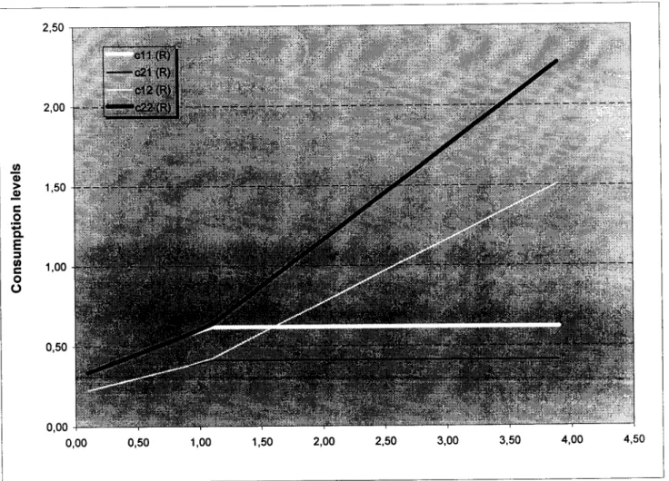
An example of the optimal contract is illustrated in figure 17. As long as r ~ 1 , the optimal allocation involves carrying over some of the liquid asset to date 2 to supplement the low returns on the risky asset in this period. When the signal indicates that R wiII be high at date 2 (Le r> 1), then the liquid asset is completely exhausted for date 1 consumption, since consumption at date 2 will be high in any case. For the parameter values of the example, the optimal levels of the initial investments are kol =0.52 and ko2 =0.48 and the expected utility achieved is -0.3757.

2.2. -Optimal risk-sharing through deposit contracts with bank runs

The optimal risk -sharing problem defined in the previous section serves as a benchmark for the risk -sharing that can be achieved in practice. It is now assumed that banks are limited to offer a standard deposit contract that

promises agents a fixed amount at each date: cll' C₂₁ for type-l and e₁₂, c

22 for type-2

8_{, and whenever that is} not possible, all available funds are divided equally among those withdrawing (as in Alien and Gale [1], it is

not assumed a sequential service constraint). In this case, when the bank is restricted to use a standard contract bank runs become a possibility. It will be denoted by 05: a(R) 5: t_{2 ,} the fraction of type-2 agents that choose to

run, or equivalently, that demand the type-l contract when the value of R becomes sufficiently small (that is, when their incentive compatiblity constraint is not satisfied). Let a be defined as follows:

a(R) =0 if (1 -p _{)lncl2 +} p _{lnC22 2} (1 -P)ln[02 Cll] + P In[(1-o_{2)cll +c21]}

a (R) > 0 otherwise

The bank chooses a portfolio kl''s., the consumption functions clj(R), c₂/R) (j= 1,2), the deposit

parameters c_lj' c_2j (j= 1,2) and the withdrawal function a(R) that maximizes the following expression:

[tl + a(R)]cll (R) + [t2 -a (R)] _Cl2 (R) d _l [t_l + a _(R)](C21 (R) + Cll (R» + [t_{2 -«(R)](C22 (R)+CI2} (R» 5:'s.R [11] (1) (2) (3) (4) (5) [tt+a(R)]clI(R)+[t2-a(R)]c12(R)=kl ifc_l1<c_l1 (7) cl/R)

s.c

lj

c

2iR)

s.c

2jR (i = 1,2) (8) Os. a(R) 5:t 2 (9)

The first five constraints are familiar. The first one states that the total amount invested must be less or equal to the amount deposited. The second constraint says that the investment in the safe asset should be enough to cover consumption at date 1. The constraint takes into account the fact that some type-2 agents may choose to run, that is, to demand the type-1 contract. The third one states that the investment in the risky asset plus the amount of the safe one that is left over from period one should be enough to cover consumption at date

explanation. As mentioned above, the bank offers individuals a fixed payment at each date _{c1j' c2j} (j

=

1, 2), although second period consumption will depend on R. If this return is sufficiently high, the contract is incentive compatible, that is, 2 agents always prefer their allocation to the possibility of receiving the type-1 allocation and using the storage technology. However, there is a critical value of R, below which, the contract is no longer incentive compatible and some or all type-2 agents will decide to run on the bank. These withdrawals will stop when the utility of the two groups is equated or equivalently. when the incentive compatibility constraint for type-2 agents is restored (constraint (6». Whenever there are runs, and therefore type-l agents cannot receive their promised payment at date 1 (c_ll), _{the bank exhausts the liquid asset among} depositors: type-l and some type-2 that demand the type-l contract (and are treated on an equal basis) and other type-2 that demand their promised payment at date 1. This is represented by constraint (7).

It is implicitly assumed that those type-2 agents that demand the type-l contract can use the storage technology, and smooth consumption in the optimal way for them, and so in equilibrium their consumption will be the same as the rest of the type-2 agents.

The solution to the bank's problem defined above is given by the following theorem:

Theorem 2.- The solution [ki>~,clJ"c2jR,cij(R), a; (R)] (j = 1,2), to the bank's problem is characterized by the following conditions: 1 kl C = -11 1 + \.I. t_lm \.I. kl C = -12 1+11 t ... Im ( A- Ptnc22 ) c ll (R) =e I-p ( l-P)B-AP) c (R) -lr R c (R) -e 1-2p 21 -"'2 22 -B=pLnk₁ +(1-p)Ln(~R) [12] [13]

if r_l<rsl (case 2): 1 kl C ( R ) = -11 1+1.1." _t lm 1.1. kl C ( R ) = -12 1 + 1.1. " _t lm 1.1. kl 1 kl c (R)=-- - r c ( R ) = - - - r 21 1 + 1.1." 22 1 + 1-1 t" tlm Im [14] if r> 1 (case 1): 1.1. kl c ( R ) = -12 1 + 1.1. " _t lm 1.1. kl 1 kl C (R) = - -

- r c

(R)

= - -

- r

21 1+1l t" 22 1+1-1" Im tlm [15] a(R) =0

" "

" tl +

t2

Il 1-1l 0: IX

and where _{t lm} = =tlm + a - - (t_{l =tl} + a, t2 =t2 - a).

1 +Il 1+1l

and kl'

kz,

the values that maximize the following expression:

[16]

Proof:

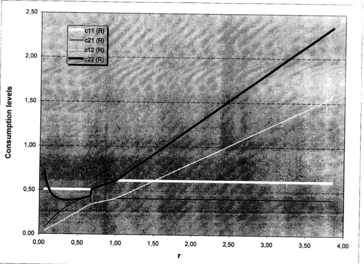
See Appendix B for a detailed resolution of the problem.

The optimal consumption levels are illustrated in figure 2, for the parameter values of the example. It can be observed that for values Of'::;;'1 =0.66 bank runs involve all type 2 agents, and the consumption levels are those given by case 3 of theorem 2. For 0.66 < r ::;; 1, bank runs will be partial and the consumption levels are those given by case 2. Finally, when

,>1

there are no bank runs and individuals will consume what was planned by the bank, as given by case 1.

If we compare the optimal consumption functions for the two problems, it can be shown that the expected utility achieved with the standard contract is always less than in the first best case. This result is expressed by the following theorem:

Theorem 3.- A banking system subject to runs can never achieve first-best efficiency using a standard contract, and therefore regulation is always needed in order to achieve the first-best.

The proof is as follows: As mentioned above, the bank offers individuals a standard contract, which is not contingent on the risky return (although second period payments will depend on it). For values of the specific return higher than one (r> 1), the contract is incentive compatible and there are no runs (a.(R) =0). In this case, the consumption functions coincide with those obtained in the first best case, in theorem 1 (notice that in this case t;'".

=

tlm)' For values of the specific return r_l <r ~ 1, the contract is no longer incentive compatible and there

would be partial bank runs, involving only a fraction of type-2 consumers (a.(R». It can be shown that

1 " ~m

substituting this value a(R), in the expression for t~m

=

t_lm + a _-_r , it is obtained

t;'".

= , and again the

1 + 1.1. t_lm +rt_2m

consumption functions given by the two theorems coincide. Finally, for very low values of the specific return, r~rl' all type-2 agents will decide to run on the bank (a(R) =t_2). This is the main difference with respect to Allen and Gale's results. In their case, due to the corner preference assumption, bank runs were always partial.

As long as there is a positive value of the

risky

asset, there must be a positive fraction of late consumers who

wait until the last period, (page 1259l. In this case, for very low, but positive values of the risky asset, bank

runs involve all type-2 consumers and are costly as they do not allow for optimal risk-sharing. Therefore, the expected utility achieved with the standard contract is always less than in the first best case.

The above result contradicts the one obtained by AlIen and Gale (theorem 2), and provides a rationale for banking regulation. In this sense, a suspension of convertibility policy, that restricts payments at date I, would implement the first-best. Payments in the first period would be restricted to a level of k<kl' where

- 1 kl

k = - - - - [ t_lm + rt_2m]. 1 +1.1. _tlm

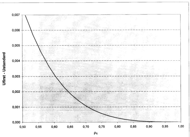
Figure 3 plots the expected utility of the first best allocation minus the standard contract as a function of p. The figure illustrates that the optimality of bank runs depends on individuals' preferences. As p -1 (AlIen and Gale's case) the difference in utility becomes zero, and hence bank runs can achieve optimal risk sharing. 3.-Concluding remarks

The motivation of this paper has been to show that AlIen and Gale's result about the optimality of bank runs depends on individuals's preferences. In a more general framework, considered in the present work, a laisse-faire policy can never be optimal, and therefore, regulation is always needed in order to achieve the first best. This result supports the traditional view that bank runs are costly and should be prevented with regulation.

Appendix A

A.- Optimal incentive compatible risk-sharing problem.

The first best allocation is obtained as a solution to the following problem:

s.t.

kl

+

kz

5.ko

tl cll (R) + t₂c_l2 (R) s.kl

tl _{[C21 (R)+cu (R)]} +~[C22(R)+CI2 (R)] S.kl +'s,R

Uj(CIj(R),c2iR)'Pj)~ [Uj(ajc]j(R),(l-a)Cli(R)+C2i(R)Pj)] for i#j; i,j=1,2

05.(\ s.1

[17]

[18]

[19]

In solving the optimal risk-sharing problem the incentive compatibility constraints can be dispensed with. The problem is solved subject to the three constraints and it can be shown that the first-best solution is always incentive compatible. For each value of R the the consumption levels ciR) solve the problem:

[20]

s.t. tl c_ll (R) + t₂c12 (R) 5. kl

[21] tl [C21 (R) + _{c ll (R)] +t2[C22 (R)+CI2 (R)]} d ₁ +'s,R

The Lagragian is formed by using the lagrangian multipliers A 1 and A2 of the two first resource constraints. The Kuhn-Tucker conditions are:

1 tl PI - --Altl +t1A2 =0 cll(R) 1 tl ( l - P I ) - - +tl A2 =0 C_{21 (R)} 1 t2 P_{2- -}-A,t_{2 +t2A2 =0} c₁₂(R) 1 t 2(l-P2) - -+t2A2 =0 c2

i

R) tl cl1(R) +t2c'2(R) -k, =0 tJ(c_l1(R) +c₂,(R)] +t₂[c,iR) +c₂₂(R)] -k,-~R Let and if cll(R) >0 if C 21(R)>0 if c,iR)>0 if c 22(R»O if )..1>0 if )..2>0

I-p

~=-­ p [a] [b] [cl [d] [f] [g] r = R

(k,.1

kl ) (t2mltlm)

This random variable r is essential in defining the ex ante risk-sharing problem. The following cases may be considered:

The optimal solution to this problem yields:

1 kl

C 11 (R) = c₂₂ (R) = - - - -[tlm + r t_2m] 1 + ~ tlm

In this case it is assumed that Al =0, or equivalently:

[22]

[23]

[24]

[25]

[26]

Substituting C;I(R) and c;2(R) in the above expression, the following condition for this case to hold is obtained,

The optimal solution is: f1 kl C ( R ) = -12 1 + f1 t_1m f1 kl 1 k\ c (R)=-- - r c ( R ) = - - - r 21 1 + f1 t_1m 22 1 + f1 t1m

In this case it is assumed AI> 0, from [a] and [b]:

1 1 A =p---(1-p)-->O 1 . • cu(R) C21(R) [27] [28]

Substituting the optimal consumption levels in the above expression we

would obtain that this case holds for

r>1.

The incentive compatibility constraints when storage is allowed are the

following ones: Type-2 agents:

c;

(R) =C₂₁ (R) _[29] Type-l agents: [30] c (R) +c (R) (b) c;(R) = 12 22 1+f1

It can be easily shown that in case 1 (r s 1), the incentive compatibility

constraints are always satisfied. In case

2 (r> 1), the incentive compatibility constraint for type-2 agents

«b»

is satisfied when n 1.

In a second step the values kl'

Is,

are obtained by maximizing the

[31]

where U*(l) and U*(2) are the utility functions corresponding to the cases r:<;; 1 and r> 1 respectively. B.- Optimal risk-sharing through deposit contracts with bank runs

The bank chooses a portfolio ki'~' the consumption functions c1iR), c2j(R) (j= 1,2), the deposit parameters c_lp c_2j (j= 1,2) and the withdrawal function a(R) that maximizes the following expression:

[32] (1) (2) (3) (4) (5) o~ a(R) ~t2 (9)

We solve the problem by parts:

Fixed payments at each date: the bank maximizes the expected utility of depositors subject to the constraints

[33]

The optimal solution to this problem yields: 1 kl C = -11 1 + _1.1. t _Im 1.1. kl C = -12 1 + 1.1. t lm - 1.1. kl 1 k, c R=----r c R=-- --r 21 1 + 1.1. t lm 22 1 + 1.1. tlm

This solution is incentive compatible for type-2 agents as long as r ~ 1 .

If r ~ 1 individuals consume what planned by the banle

If r_l ~r< 1 there will be partial bank runs, as some type-2 agents will claim the type-l contract. [34]

Let a(R) be defined as the proportion of type-2 agents that choose to run. These withdrawals will stop when the incentive compatibility constraint is restored, that is,

a(R) is S.t. ra. = 1

~ t~m

where ra. =R--k ta. 12m a. 1-11 tl =t +a(R)--m Im 1 +1.1.

Solving for a(R) in the above expression yields:

1 1 + [ t -t r

1

a(R) = -

---..!:

t - t + Im 2m ~ t 2 1 - 2m Im t + t r 2 1.1. lm 2m [35] [36]

Consumption of individuals in each period would be obtained by maximizing the expected utility subject to the constraints:

[t_l +a(R)] c_l1(R) + [t₂ -a (R)] C₁₂(R)

=

kl

[t_l +a(R)] c₂₁(R) + [t₂ -a(R)] C₂₂(R) = ~R

and incentive compatibility constraints «5) and (6». with solution: 1 kl c_l1 (R) = -1+1.1. ta. lm 1.1. kl C ( R ) = -12 1 + 1.1. tU lm 1.1. kl 1 kl C 21(R)=-- --r _{1 + 1.1. ta.} c ( R ) = - - - r 22 1 + 1.1. ta. lm Im [37] [38]

t

a(R) 5 t₂-nq.L ~

=

r_l and so for values of r<r_l bank runs will involve all type-2 agents. t2m

If r<r_l all agents will run on the bank and so in this case the constraints would become:

and the optimal consumption levels,

c_{l l}(R) =k_l C₂₁(R) =k₂R where A = (1-p)Ln(kl

+~R)~)+

P

7j_kl_+_~_R)

1+~

J..I"\

1+~

B=pLnkl +(l-p)Ln(~R) [39] [40]

In a second step, the optimal levels of the initial investments (ki' ~) are the values that maximize the following expression:

[41]

It remains to be shown that when _r<rl suspending convertibility a level k<kl implements the first best. In this case the bank would maximize the expected utility subject to the following constraints:

[42]

and incentive compatibility «5) and (6».

In this case, the bank does not exhaust the liquid asset and so the suspension level would be

- 1 kl

k = - - - -[tlm + rt_2m] and the optimal consumption levels: 1 +~ t_lm

as in the first best case.

References

1.- Alien, F. and D. Gale, 1998, Optimal financial crises, Journal of Finance 53, 1245-1284.

2.- Bhattacharya, S. and D. Gale, 1987, Preference shocks, Liquidity and Central Bank Policy, New Approaches to Monetary Economics, WA, Barnett and K.J Singletons (eds). Cambridge University Press, 69-88.

3.- Chari, V. and R. Jagannathan, 1988, Banking Panics, Information and Rational Expectations Equilibrium, Journal of Finance 43(3), 749-761.

4.- Diamond, D. and P. Dybvig, 1983, Bank Runs, Deposit Insurance and Liquidity, Journal of Political Economy 91(3), 401-419.

5.- Gorton, G. 1988, Banking panics and business cycles, Oxford University Press.

6.- Jacklin, C. 1987, Demand Deposits, Trading Restrictions and Risk Sharing, E.C Prescott and N.Wallace (eds.), Contractual Arrangements for Intertemporal Trade, University of Minnesota Press 26-47.

7.- Jacklin, C. and S. Bhattacharya, 1988, Distinguishing Panics and Information-based Bank Runs: Welfare and Policy Implications, Journal of Political Economy 96, 568-592.

8. - Samartin, M. 1997, Financial intermediation and public intervention, PhD dissertation, Core, Universite Catholique de Louvain.

III

a;

2,50 2,00 ~ 1,50 c

o

;: c..

E

~ ~ 1,00

o

o

0,50 0,00 0,00 0,50 1,00 1,50 2,00 2,50

Figure 1.- Optimal consumption levels in the first best allocation

R

r C11 C12 ~1 0,100 0,094 0,339 0,226 0,226 0,300 0,281 0,397 0,265 0,265 0,500 0,468 0,455 0,303 0,303 0,700 0,656 0,513 0,342 0,342 0,900 0,843 0,571 0,381 0,381 1,100 1,030 0,620 0,413 0,426 1,300 1,218 0,620 0,413 0,503 1,500 1,405 0,620 0,413 0,580 1,700 1,592 0,620 0,413 0,658 1,900 1,780 0,620 0,413 0,735 2,100 1,967 0,620 0,413 0,813 2,300 2,154 0,620 0,413 0,890 2,500 2,342 0,620 0,413 0,967 2,700 2,529 0,620 0,413 1,045 2,900 2,716 0,620 0,413 1,122 3,100 2,904 0,620 0,413 1,199 3,300 3,091 0,620 0,413 1,277 3,500 3,278 0,620 0,413 1,354 3,700 3,465 0,620 0,413 1,432 3,900 3,653 0,620 0,413 1,509 3,00 3,50 4,00 4,50 C22 0,339 0,397 0,455 0,513 0,571 0,638 0,754 0,871 0,987 1,103 1,219 1,335 1,451 1,567 1,683 1,799 1,915 2,031 2,147 2,263

tn Q) > .,S! c: 0 ;; c.

E

:l (1) c: 0 0 2,00 1,50 1,00 0,50 0,00 0,00 0,50 1,00 1,50 2,00 r

Figure 2.- Optimal consumption levels with the standard contract

R r a C11 C12 0,100 0,096 0,500 0,510 0,098 0,300 0,289 0,500 0,510 0,266 0,500 0,481 0,500 0,510 0,371 0,700 0,674 0,487 0,512 0,341 0,900 0,866 0,179 0,571 0,380 1,100 1,059 0,000 0,611 0,408 1,300 1,251 0,000 0,611 0,408 1,500 1,444 0,000 0,611 0,408 1,700 1,636 0,000 0,611 0,408 1,900 1,829 0,000 0,611 0,408 2,100 2,022 0,000 0,611 0,408 2,300 2,214 0,000 0,611 0,408 2,500 2,407 0,000 0,611 0,408 2,700 2,599 0,000 0,611 0,408 2,900 2,792 0,000 0,611 0,408 3,100 2,984 0,000 0,611 0,408 3,300 3,177 0,000 0,611 0,408 3,500 3,369 0,000 0,611 0,408 3,700 3,562 0,000 0,611 0,408 2,50 3,00 3,50 4,00 ~1 C22 0,049 0,580 0,147 0,391 0,245 0,395 0,341 0,512 0,380 0,571 0,432 0,647 0,510 0,765 0,589 0,883 0,667 1,001 0,746 1,118 0,824 1,236 0,902 1,354 0,981 1,471 1,059 1,589 1,138 1,707 1,216 1,825 1,295 1,942 1,373 2,060 1,452 2,178

-l

0,007 - , - - - , - - - _I 0,006 0,005 0,004 0,003 0,002 0,001 0,000 +----,--...-.-:~--...,..__--...,._~-...,._--_,__--=:::::;=~"""""_--__,__-~ 0,50 0,55 0,60 0,65 0,70 0,75 0,80 0,85 0,90 0,95 1,00 Pi

Notes

1. See Samartin {8] for a detailed description of bank regulation in the US and Europe in the 20th century.

2. It should be noticed that mast deposit insurance systems in Europe were created in the 1970s.

3. In the madel, panic runs may occur due to the fact that uninformed individuals condition their beliefs about the bank's long-term technology on the size of the withdrawal queue at the bank. If this size is large (due to a high liquidity shock only) they may nevertheless infer sufficiently adverse information to precipitate a bank run.

4. Another exception is Bhattacharya and Gale [2] or a few other references mentioned in Allen and Gale {l}.

5.

Allen and Gale {I] follow the Diamond and Dybvig {4] specification of preferences, in which individuals derive utility for consumption either in period 1 or in period 2. However, as Jacklin {6] has noted, this assumption on preferences has the feature that banks and morkets are equivalent risk sharing instruments, and therefore this rules out a positive role for a financial intermediary.

6. The incentive compatibility constraints are derived in more detail in Appendix A.

7 .In the numerical example, a triangular distribution for the random variable has been assumed.

8. Note that the standard contract is noncontingent on R, although the feasibility constraints will make second period payments depend on it.

9.It should be noticed that in Allen and Gale's case TI = I.L tlm = 0 as I.L = I-p =0 and therefore bank runs are always partial.