From Constant to Stochastic Volatility: Black-Scholes Versus Heston Option Pricing Models

(1)

Bard College Bard College

Bard Digital Commons

Senior Projects Spring 2019 Bard Undergraduate Senior Projects Spring 2019

From Constant to Stochastic Volatility: Black-Scholes Versus

Heston Option Pricing Models

Hsin-Fang Wu

Bard College, hw7415@bard.edu

Follow this and additional works at: https://digitalcommons.bard.edu/senproj_s2019 Part of the Other Mathematics Commons

This work is licensed under a Creative Commons Attribution-Noncommercial-No Derivative Works 4.0 License. Recommended Citation

Recommended Citation

Wu, Hsin-Fang, "From Constant to Stochastic Volatility: Black-Scholes Versus Heston Option Pricing Models" (2019). Senior Projects Spring 2019. 163.

https://digitalcommons.bard.edu/senproj_s2019/163

This Open Access work is protected by copyright and/or related rights. It has been provided to you by Bard College's Stevenson Library with permission from the rights-holder(s). You are free to use this work in any way that is permitted by the copyright and related rights. For other uses you need to obtain permission from the rights-holder(s) directly, unless additional rights are indicated by a Creative Commons license in the record and/or on the work itself. For more information, please contact

(2)

From Constant to Stochastic Volatility:

Black-Scholes Versus Heston Option Pricing

Models

A Senior Project submitted to

The Division of Science, Mathematics, and Computing

of

Bard College

by

Hsin-Fang Wu

Annandale-on-Hudson, New York

May, 2019

(3)

(4)

Abstract

The Nobel Prize-winning the Black-Scholes Model for stock option pricing has a simple formula to calculate the option price, but its simplicity comes with crude assumptions. The two major assumptions of the model are that the volatility is constant and that the stock return is normally distributed. Since 1973, and especially in the 1987 Financial Crisis, these assumptions have been proven to limit the accuracy and applicability of the model, although it is still widely used. This is because, in reality, observing a stock return distribution graph would show that there is an asymmetry or a leptokurtic shown in the stock return.

Therefore, we propose that by introducing the Heston Model, we can tackle these two prob-lematic assumptions in the Black-Scholes Model. The Heston Model considers the leverage effect and the clustering effect, which allows the volatility itself to be random and also allows it to take the non-normally distributed stock return into account.

In our project, we aim to show whether the Heston model can actually improve the option pricing estimates by using theS&P 500 Index European Call Option to compare it to the Black-Scholes Model. We find that even though the results show that the Heston Model performs worse than the Black-Scholes Model when the option expiration date is soon to expire, the Heston Model significantly outperforms the Black-Scholes Model in almost all combinations of moneyness and maturity scenarios. There remains further work to improve the Heston Model.

(5)

(6)

Dedication

I want to dedicate this project to my parents in Taiwan, Anna Cheng and Tai-Ju Wu. I am really grateful for their supports, love, and encouragements. I am really appreciated that I have very wonderful parents who give so many guidelines and always supports me to do a lot of different things. I really appreciate that I decided to come to Bard to study both math and music in 2015. It is a very tough program, but I really learn so much at Bard. I grow so much and learn how to find my own path here. I am glad that I make it to the place where I am today. I hope I can dream higher and be more fearless in trying and learning different new things in my life.

(9)

(10)

Acknowledgments

I thank for my advisor, Stefan for working with me on this topic. I thank my parents for their endless supports and love. I thank Jane for always helping me when I need the supports, thank for Paul meeting with me to improve my project, and thank professor Li on the other side of the world to answer my questions and provide the guidelines. I cannot finish this project without my beloved two friends Alisa and Corrina. We have too many memories throughout the 4 years at Bard. I appreciate all these supports I got from Bard. I thank for professor Gautam for suggesting this topic for me. This really opens a new door for me and I would like to explore more applied math in finance and consider working in quantitative finance. At last, I thank Michael, for always being by my side, supporting me and encouraging me when I am down.

(11)

(12)

1

Introduction

The purpose of my project is to compare the accuracy of two financial models–the Black-Scholes-Merton (BSM) model and the Heston Model–that are used to estimate the price of an option. I will give an example of what a call option is first and will move into the backgrounds of these two models.

Imagine one day that you cannot wait to get the new iPhone for your little brother for Christmas, but the store is running low on stock and you are afraid the price will go up. And you only have budget of $200 and the price of the iPhone is $220. Someone unknown comes up to you and says “if you give me $4, I can guarantee that you can buy the new iPhone on December 21st for $195.” If on December 21st, the price is cheaper than $195, you will just buy it directly from the market since the price is cheaper than $195 offered by the stranger. In this case, you will just lose $4 for accepting this stranger’s offer.

Paying the $4 is called buying a call option. Call options are a formal contract between a buyer and a seller. The holder of a call option (in this case, you) has the right, but not the obligation, to buy a commodity at a specified price on a specified date. Options are important not only because they can serve as an insurance to protect your investment when the market is not doing well but also you can own a commodity without really paying the actual commodity price until the option expires. This saves you money and you can use that money to make other

(13)

2 INTRODUCTION

investments. Thus options are very a flexible and powerful tool for investors to make money from the market.

In my example, the price of the commodity is $220, the maturity is December 21st, and the price which you (the buyer) and the stranger (the seller) agree on while you accept the offer (called a strike price) is $195. If all these quantities are fixed, the question becomes what is a fair price for the option? If we can have a way to calculate a fair option price, then we can see whether the option price being offered (in this case, $4) to you is worth it or not before you agree to buy the option.

The Black-Scholes-Merton (BSM) model for option pricing was developed by Fischer Black, Myron Scholes and Robert Merton in 1970s. This impacted the financial world because it became possible to price options using a relatively simple explicit closed-form formula provided by the BSM for the first time. But this simple model comes with many assumptions that are not consistent with what is observed in the financial market, which we will explain later on. This model is still widely used not just because it becomes the standard and traditional way to calculate the , and was awarded the 1997 Nobel Prize in Economics. But also it is easy to implement. If everybody is using the BSM to price options, it make sense to take a look at what assumptions this model are based on and how the model is implemented.

There are only five parameters needed for the BSM to estimate the, which are stock price, strike price, interest rate, maturity date, and implied volatility (the standard deviation or the amplitude) of the stock. The five parameters are represented mathematically as follows:

BSM(stock price, strike price, interest-rate, maturity, σ) = theoretical option price

The output of the BSM, in its initial formulations, gives a theoretical option price that is not rooted in realistic situations. The first four parameters, stock price, strike price, interest rate, maturity, are observable market data. These variables can be easily determined by looking at market data. The only parameter left, σ, represents the implied volatility of the stock return, which is not easily observable in the market. Thus the way to solve the implied volatility is to set the market price as the fair option price and to solve the BSM backward to find the appropriate

(14)

INTRODUCTION 3

σ that makes the output of the BSM equal to the market . That is why it is called “implied” volatility because it is the value that is implied by the market option price.

But the simplicity of the formula comes with crude assumptions. I will mainly deal with two major assumptions in the BSM in this project–the constant stock volatility (a measure of how far the stock return is from the mean; the standard deviation) and the lognormal stock returns (the normal distribution,or bell-curved distribution, of the log stock returns). As described in [1], since the 1987 stock market crash, these assumptions have been proven wrong. A volatility smile or skew observed in the market shows that the BSM assumption on constant volatility is wrong.

As pointed out in [3], the volatility smile is the consequence of the lognormal stock return assumptions in BSM proposed by John C. Hull and Nattenburn. Also the stock return in the real market is actually not normally distributed. There are asymmetry and fat tails (the longer tails extended on the both sides of the distribution) shown in the stock return distribution as mentioned in [3]. It is obvious that both the constant volatility and the lognormal stock return in the BSM cannot represent the real financial market. The question becomes how to price options in a way that takes the real financial market into account.

One of the approaches to tackle this problem is to allow the volatility to be random, or stochastic. There have been many models proposed for stochastic volatility. But Heston remains one of the most popular ones due to its closed-form solutions for the European options. Scott (1987), Hull and White (1987), Wiggins (1987) generalized the model to allow volatility as a stochastic process. However, as described in [4], their models require quite an amount of numerical computations and do not really take into account the fact that volatility is correlated with stock returns.

In 1993, the Heston Model was developed by Steven Heston. It provides a stochastic model that extends the BSM. It addresses both the constant volatility and the lognormal stock returns assumptions by relaxing these assumptions. It allows the volatility itself to be a random variable and also allows the log of stock returns to be nonstandard normal distribution. By allowing

(15)

4 INTRODUCTION

non-constant volatility and non standard normal distribution of the stock returns, the Heston Model can take the asymmetry, the fat tails observed in the stock return distribution, and the volatility smile into account.

As described in [28], the Heston Model assumes both the stock price and the variance of the stock price follow the Brownian motions (a random, or stochastic process). And these two Brow-nian motions are correlated. In reality, the correlation is usually negative in the equity world. That means increases/decreases in the stock price tend to be coupled with a decrease/increase in volatility, which is called the leverage effect in finance. Besides taking into account the corre-lation between stock price and volatility, the main attraction of the Heston Model is its closed-form solution. This makes the calibration of the model feasible as described in [6]. The Heston parameters can be obtained by calibrating to market data. We used the lsqnonlin nonlinear least-squares optimization method in MATLAB to calibrate the Heston Model in the project.

Besides thelsqnonlin method, there are many different optimizations for calibrating the He-ston Model, including but not limited to the Adaptive Simulated Annealing(ASA), Generalized Reduced Gradient, and Genetic Algorithm(GA). All calibration algorithms search for a region of the parameters while trying to minimize the error metrics. We can see [24] and [28] for more detailed information about using different optimisations to calibrate the Heston Model. But both [24] and [28] prove the lsqnonlin nonlinear least-square method in MATLAB is faster in obtaining the five unknown parameters in the Heston Model, and that the five unknown param-eters obtained by using the lsqnonlinmethod generate more accurate option prices among the other optimizations.

In this project, we need to deal with a total of 3,774 S&P 500 Index European call option data for the whole month. Thus we choose lsqnonlin due to its speed and accuracy. But the method is sensitive to the choice of the initial point. The way to address the sensitivity is to define the range of acceptable solutions, which at least guarantees that the solutions are not just mathematically feasible but also make sense economically.

(16)

INTRODUCTION 5

My main focus will be the comparison of the estimates given by the Heston Model, the Black-Schoels model, and the actual market option price from iVolatility.com. I use the mean absolute percentage error (MAPE) as my accuracy comparison criteria. The smaller the number is, the more accurate it is. My results show that the Heston Model is more accurate than the BSM in estimating theS&P 500 Index European call option price.

It is worth mentioning that most of the papers testing the accuracy of the BSM and the Heston Model do not use enough data sets to calibrate the Heston Model. They only choose certain segments of data sets without fully taking all possible scenarios into account. Thus their calibration processes are less time-consuming and easier because they do not use enough market data to calibrate the Heston Model. Thus the five unknown parameters (initial volatility, long-term volatility, mean-reversion speed, the correlation between stock price and volatility) cannot fully explain the market behaviors, even though the results might still show that the Heston is more accurate in predicting option prices compared to the BSM.

Thus we want to consider as many scenarios as possible in trading European call options. So I use a total of 3,774S&P 500 Index European call options which covers a total of 96 different maturities and of 98 different strike prices traded in the market from February 4th to March 4th in 2019 to calibrate the Heston Model in order to accommodate more trading call option situations by using more different maturities and strike prices. This is not an easy task because I use a larger amount of data compared to many papers which only use less than 300 data to run the results. I divide a total of 3,774 data into 15 files; each file represents one scenario depending on the combination of moneyness (the degree of whether you make money or lose money) and maturities. By doing this, I can show a clearer picture of how both models perform under these 15 different scenarios. It is worth mentioning that using the whole month data to calibrate the Heston Model requires a great deal of computer memory than a standard Macbook to find the five unknown parameters. I needed to run the algorithm on an iMac in the lab since a standard Macbook crashed due to lack of memory. Thus the whole process for analyzing the whole day data traded in the market is quite time-consuming.

(17)

6 INTRODUCTION

Many researchers only use a few maturities and strike prices to calibrate the Heston Model, and use the five unknown parameters obtained from the calibration in the Heston Model to estimate the option prices. But, without using enough data sets to calibrate the Heston Model, the results can only reflect the behavior of the market under those segments of data, which fails to give more realistic and more accurate estimations that take enough trading situations into account. Thus in my project, we try to take more different strike prices and maturities into account and hope to obtain the five unknown parameters that reflects more different trading situations observed in the market into account by using the whole month S&P 500 Index European call option data. After obtaining these five parameters, we use them afterwards in the Heston Model and compare the Heston’s estimates, the BSM’s estimates and the real market data for a total of 3,371 call options traded on March 19th in 2019.

The purpose of my project is to compare the accuracy of the BSM and the Heston Model. Thus our focus will be on the implementation of these two models. For the details of the derivation of these two models, see [2] and [4]. For the data, we will mainly deal with S&P 500 Index European call options. The basic concepts for the options will be presented in Chapter 2.

1.1

Method

To test the accuracy of the BSM and the Heston Model for Index, I first obtained the data from iVolatility.com on March 19th , which includes stock price, maturity, strike price, mid price, bid price, ask price and implied volatility. For the interest rate, I looked up 1-year yields from the treasury.gov. I filtered out the data with too short or too long maturities, negative volatility, and the very deep-in-the-money (the position where you make a lot of money from the options) and very deep-out-of-the money (the position where you lose a lot of money), since these cases are quite rare and short-lived in the market. I was left with 3, 371 call options with a total of 23 maturities and a total of 103 different strike prices. I categorized them into 15 files in Excel depending on their maturity and the moneyness.

(18)

1.2. STRUCTURE 7

It is a lot easier to implement the BSM since it has simple formula and it does not require extra calibration before implementing the model as the Heston Model does. Thus for the BSM, we use the MATLAB code in the Appendixbsm callto estimate theS&P 500 Index European call options under the BSM. But for the Heston Model, it requires a calibration process to find the five unknown parameters which I will introduce later. Once obtaining the five unknown parameters, we have all the input parameters needed in the Heston Model and thus can implement the Heston Model using the functioncall heston cf in MATLAB (see Appendix A).

The approach for the calibration process is to calibrate the Heston Model to the real market data to obtain the five unknown parameters, which are the initial volatility (V0), the long-term volatility ( ¯V), the volatility of the variance process (η), the mean-reverting speed for the volatility process (a), and the correlation between the stock price and the volatility (ρ). For the calibration data, I obtained one month ofS&P 500 Index European call options from iVolatility.com from February 4th to March 4th in 2019. I filtered out the negative volatility, too short, too long maturity, very deep-in-the-money and very deep-out-of-the-money. I was left with 3,774 call options with a total of 96 different maturities and a total of 98 different strike prices. I used thelsqnonlinnonlinear least-square method in MATLAB to search for the parameters by minimizing the squared error between the model price and the market price. Once I had the five parameters, I plugged those values into call heston cf in MATLAB to estimate the values of the option prices. Finally, we can compare the estimates of the Heston Model and the estimates by the BSM to the market data we obtained on March 19th by using the forecast error called the mean absolute percentage error (MAPE).

1.2

Structure

This project is divided into the following chapters. In Chapter 2, we introduce the basic finance concepts and the Black-Scholes Model, but the attention will be given to the volatility and the limitations of the BSM, which will lead to the assumptions of the Heston Stochastic Volatility Model. In Chapter 3 , we introduce the Heston Stochastic Volatility Model and discuss the

(19)

in-8 INTRODUCTION

fluence of the five missing parameters in the Heston Model in great detail. The ways to obtain these missing five parameters will require the calibration process. Thus in Chapter 4, we intro-duce the different optimizers to calibrate the Heston and uses the standard approach–lsqnonlin

nonlinear least-squares method in MATLAB–to calibrate the Heston Model in order to obtain the five missing parameters. In Chapter 5, we present the results in the comparison of the accu-racy between the BSM and the Heston Model using mean absolute percentage error (MAPE). Chapter 6, we present the conclusion and discuss what further work remains to be done in order to improve my results. Appendix A contains all the MATLAB codes used for the calculations throughout the project.

1.3

Terminology

The following terms and notations will be used a lot in the project, but will be explained fully in the following chapter. This section is mainly cited from [33].

• Call,C: An option that gives the holder the right to buy a share of stock on a given date at a predetermined price.

• Put, P: An option that gives the holder the right to sell a share of stock on a given date at a predetermined price.

• Strike Price, K: The price at which the holder can buy or sell the underlying stock.

• Expiration data or Maturity date, t: The date at which the underlying stock is selling at datet.

• Option price: The price at which the option is sold or bought.

• Risk-free interest rate,r: The rate of of an investment with no risk of financial loss, over a given time period.

(20)

2

The Black-Scholes Option Pricing Model

In this chapter, we introduce the finance terms and the basic financial concepts that are fun-damental to the Black-Scholes Merton (BSM) model and the Heston Model. In this project, we only focus on pricing European call options in order to align with the BSM assumption in options being European style, or European options. In brief, European options only can be exercised on the expiration date, whereas American options can be exercised before, or on, the expiration date. The main attention will be drawn to the Black-Scholes Model session and its limitations session.

2.1

Derivative Contracts

Derivatives are contracts based on the the underlying asset price. They can be applied to almost any types of asset such as oil, gasoline, gold, commodity and stocks. In this project, we will focus on derivatives based on stocks. That is stock options. Thus we will introduce the definitions of stock and stock return first, and the main attention will be given to European call options. This section is mainly cited from [7], [13], [8], [27], and [34].

(21)

10 2. THE BLACK-SCHOLES OPTION PRICING MODEL

Definition 2.1.1. As described in [7], A stock also known as “shares” or “equity” is a type of security that signifies proportionate ownership in the issuing corporation. This entitles the

stockholder to that proportion of the corporation’s assets and earnings. 4

Definition 2.1.2. Let P0 be a stock price at initial buying time, let P1 be stock price at sell time, and let D be the dividends. The stock returns means the net lost or gain made on an investment, which is given by the formula

Total Stock Return = (P1−P0+D)

P0

.

4

Definition 2.1.3. As described in [13],optionsare financial derivative sold by an option writer to an option buyer. They are typically purchased through online or retail brokers. The contract offers the buyer the right, but not the obligation to buy or sell the underlying asset at an agreed

upon price under a certain period of time or on a specific date. 4

Definition 2.1.4. A European call option is a contract that gives its holder the right, but not the obligation, to buy one unit of a stock S for a specified price also known as strike price

K on a time maturity dateT but not before or after time maturity date T.

A European put option is a contract that gives its holder the right, but not obligation, to sell one unit of a stockS for a specified strike priceK on a time maturity dateT but not before or after time maturity date T.

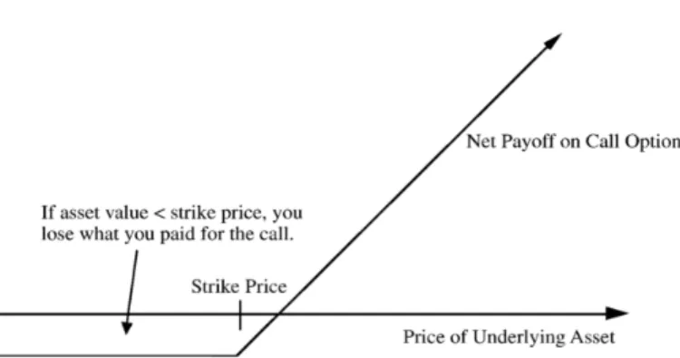
The payoffs for the European call option and put option are given by

Call =

(

(ST −K)−call option price forST > K

call option price forST ≤K

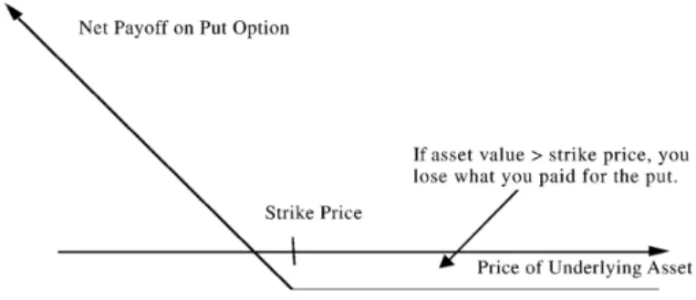
and for the European put option in the analogous way

Put =

(

put option price + (K−ST) forST < K

put option price forST ≥K.

(22)

2.1. DERIVATIVE CONTRACTS 11

Example 2.1.5. Consider an investor who buys a European call option contract on Apple stock with a strike price $100 to purchase 100 shares of the stock. Suppose that the current stock price is $100, the maturity date of an option is in 3 months, and the price of this option to purchase one share is $2.00. The initial investment of buying this call option is $100×$2 = $200. Since it is European call option, the investor can exercise the option only on the maturity date. We divide our scenario into two cases.

• Scenario one: When the option expires, Apple is trading at $105.

The call option gives the buyer the right to purchase those shares at $100 per share. In this scenario, the buyer could use the option to purchase those shares at $100, then immediately sell those same shares in the open market for $105. The buyer can immediately gets additional $5 per share and make the total extra $5×$100 = $500. Since the investor purchased this option for $200, the total payoff to the buyer is ($105−$100)×100 shares−

$200 = $300.

• Scenario two: When the option expires, Apple is trading at or below $100.

The investor will clearly choose not to exercise and let the contract expire worthless. So the investor will only lose the $200 initial investment.

♦

(23)

12 2. THE BLACK-SCHOLES OPTION PRICING MODEL

Figure 2.1.2. Payoff on Put Option

Definition 2.1.6. Moneynessis the relationship between the strike price of an options contract and the price of the underlying security at the time of maturity. The followings main three terms are in terms of call options.In-the-money means when underlying stock price of an option is higher than the strike price of the option.At-the-moneymeans when strike price is equal to the underlying stock price of an option. Out-of-the-Money means the strike price is higher than the underlying stock price of an option. For put options, they will have the opposite relationship. The moneyness for call options is defined as the percentage difference between the stock price (S) and the strike price (K):

moneyness = S

K −1.

4

Moneyness serves as an important criteria when you are an option trader. For example, if you are buying option contracts on an underlying asset that you are expecting to move dramatically in price in a short time, then buying out-of-the-money contracts would maximize your potential profits. If you are expecting smaller movement, then in-the-money contracts would probably represent a better, less risky investment. [8] provides further information.

2.2

Black-Scholes-Merton model

The Black-Scholes-Merton (BSM) model was developed in 1973 by Fischer Black, Robert Merton, and Myron Scholes and is still widely used today. BSM is the first pricing model used to determine the theoretical value for European call options. It is based on five input parameters: stock price

(24)

2.2. BLACK-SCHOLES-MERTON MODEL 13

S, strike price K, maturityt, risk-free interest rater and implied volatility of stock returns, or standard deviation of stock returnσ.

BSM has become the common language among option traders. It is regarded as the benchmark to determine option prices due to the fact that it is the most standard and traditional option pricing model, it has the simplest formula and it is easy to implement. Option traders use the BSM to buy call options priced higher than the BSM and sell options that are priced higher than the BSM.

2.2.1 Black-Scholes Formula

LetC be the European call option price,S be the current stock price,K be the strike price,r

be the risk-free interest rate, σ be the standard deviation of the logarithm of stock return, or implied volatility,tis the maturity,N be the standard normal cumulative distribution function with mean 0 and standard deviation 1 and N(d) be the value of the cumulative standardized normal distribution evaluated at d1 andd2.

The The Black-Schoels Model Formulafor European call options is defined as:

C(S, K, σ, t, r) =SN(d1)−Ke−rtN(d2) (2.2.1) where N(z) = Z z −∞ 1 √ 2πe −z2 2 for all−∞< z <∞, d1 = log(_KS) + (r+σ₂2)t σ√t d2= log(_KS) + (r−σ2 2)t σ√t =d1−σ √ t

andN(d1) and N(d2) are probability factors.

2.2.2 Explanations for the Black-Scholes Formula

This section is consulted from [25]. e−rt is the present value factor, and reflects the fact that the strike priceK on the call option does not have to be paid until expiration. The termKe−rt

(25)

14 2. THE BLACK-SCHOLES OPTION PRICING MODEL

price will be at or above the strike price when the option expires. In other words, N(d2) is the probability that the option will be exercised. Therefore, the term Ke−rtN(d2) means the strike price discounted back to present value times the probability that the option is at or above the strike price when the option expires.

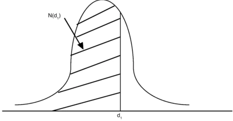
N(d1) is roughly, looking for the area under the bell curve up tod1. See Figure 2.2.1. N(d1) can also be interpreted as the probability that the future price will be above the strike price on the expiration date. See Nielsen [30] for the more details about N(d1) andN(d2).

In general, we can view SN(d1) as how much you get for exercising this option, or return. We can viewKe−rtN(d2) as how much you pay for the option, or the cost of the option. Thus

SN(d1)−Ke−rtN(d2) is the total profit you get minus the total cost of the option. Roughly, it is an investor’s return minus the cost of the option.

Figure 2.2.1. Cumulative Normal Distribution

2.2.3 The BSM Assumptions

When the Black-Scholes Formula was published, it was under the following assumptions. This section is mainly cited from [19].

1. The stock priceS follows a stochastic process, geometric Brownian motion,dS=µSdt+

σSdz, with constant driftµ, standard deviation of the stock returnσ anddz is a standard Wiener Process.

(26)

2.2. BLACK-SCHOLES-MERTON MODEL 15

2. The stock return involving in the computation of the Black-Scholes formula is log-normally distributed with constant mean and variance rates.

3. No traction costs and no taxes;

4. No dividends are paid during the life of the options;

5. There are no risk-less arbitrage opportunities;

6. Based on European options;

7. Continues trading;

8. The risk-free rate of interestr is constant for different maturities.

.

2.2.4 BSM Parameters

The value of a European call option in the BSM is determined by five parameters relating to the commodity and financial markets. The details for each parameter is presented. This section is cited from [34].

1. Current Stock PriceS

Options are assets that derive value from an underlying asset (stock). Therefore, changes in the value of the underlying asset affect the value of the options on that asset. Since call options provide the right to buy the underlying asset (stock) at a fixed price (strike price), an increase in the value of the asset will increase the value pf the call options. Puts, on the other hand, become less valuable as the value of the asset increases.

2. Implied Volatilityσ

Implied Volatility represents the standard deviation. The buyer of an option acquires the right to buy or sell the underlying asset (stock) at a fixed price. The higher the standard deviation in the value of the stock, the greater the value of the option. This is true for both

(27)

16 2. THE BLACK-SCHOLES OPTION PRICING MODEL

calls and puts. While it may seem counterintuitive that an increase in standard deviation should increase value, options are different from other derivatives since buyers of options can never lose more than the price they pay for them; in reality, they have the potential to ear significant returns from large price movements.

3. Strike PriceK

Strike price is the price that the buyers and the sellers agree to buy or sell. In the case of call options, where the holder acquires the right to buy at a fixed price, the value of the call will decline as the strike price increase. We can see from Equation 2.2.1. If theSN(d1) stays the same, the increase in the K−rtN(d2) will decrease the output of the BSM. In other words, the call option value will become less.

4. Time to Expiration, or Maturityt

Both calls and puts are more valuable, when the maturity is greater. This is because the longer time to expiration provide more time for the value of the underlying asset (stock) to move, increasing the value of both types of options. Besides, in the case of call, where the buyer has to pay a fixed price at expiration, the present value of this fixed value decrease as the life of the option increases, increasing the value of the call.

5. Risk-free Interest Rate r

Since the buyer of an option pays the price of the option up front, an opportunity cost is involved. This cost will depend on the level of interest rate and the time to expiration of the option. The risk-free interest rate also enters into the valuation of options when the present value of the strike price is calculated, since the strike price does not have to be paid (received) until expiration on calls or puts. Increase in the interest rate will increase the value of calls.

(28)

2.3. IMPLIED VOLATILITY–THE ONLY MISSING PARAMETER IN THE BSM 17

2.3

Implied Volatility–The Only Missing Parameter in the BSM

The Black-Scholes Model requires only five inputs into the model. These five inputs are stock price (S), strike price maturity (K), maturity (t), risk-free interest rate (r), and standard devi-ation of the stock return (σ), or implied volatility. The formula for the BSM can be expressed as

BSM(S, K, t, r, σ) = Theoretical Call Option Price.

The first four parameters S, K, t and r are easily observable in the market. They can be determined by looking at the market data. The only missing parameter in the BSM is the standard deviation of the stock return,σ, which is not observable in the market. To calculate

σ, we first make the BSM equal to the market price and then solve the equation backwards to find the appropriateσ that makes the equation equal to the option market price.

In other words, implied volatility is the value of the volatility parameter σ that must go into the BSM formula (see Equation 2.2.1) to match the market price:

BSM(S, K, t, r, σ) =Cmarket (2.3.1)

where Cmarket is the easily observable market call option price, S is the stock price, K is the strike price,t is the maturity, r is the risk-free interest rate and σ is the implied volatility, or standard deviation of stock return.

As we have seen thatimplied volatility is the value we get from equating the option market value to its BSM value. It reflects the volatility suggested by the market and also tells us how volatile the stock would be in the future.

2.3.1 The Newton-Raphson method

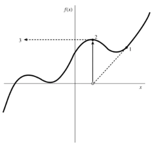
This section is mainly cited from [36]. One of the most efficient algorithms to estimate the implied volatility from the market observed price and the theoretical Black-Scholes formula is the Newton-Rahpson method. Newton-Raphson method is used to find the zeros of a real valued function. This means if there is a function f(x), then the root of the function would

(29)

18 2. THE BLACK-SCHOLES OPTION PRICING MODEL

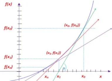
be such that f(x) = 0. The Newton Method is well suited on computers because it is iterative in nature. This feature of Newton-Raphson method has attracted many scientists and many scientific application programs use Newton-Raphson method as one of the root finding tools. The Newton-Raphson methodin one variable is implemented as follows:

Given a function f(x) defined over the real x, and its derivativef0(x) , we begin with a first guess x0 for a root of the functionf. Provided f0(x)6= 0, a better approximation x1 is

x1=x0−

f(x0)

f0₍_x

0)

.

Geometrically, (x1,0) is the intersection with the x-axis of a line tangent to f at (x0, f(x0)). The process is repeated as

xn+1 =xn−

f(xn)

f0₍_x

n)

(2.3.2)

until a sufficiently desired accurate value is obtained. See Figure 2.3.1 for the geometric inter-pretation of Newton-Raphson Method.

Figure 2.3.1. Geometric Interpretation of Newton-Raphson Method

2.3.2 How to apply the Newton Method to calculating the implied volatility?

In order to apply the Newton method to calculating the implied volatility, we need to find a functionf(σ) so we can use the Newton method to find theσ such thatf(σ) = 0. We can view the BSM as a function called BSM(σ) which only depends onσ, provided that the other four

(30)

2.3. IMPLIED VOLATILITY–THE ONLY MISSING PARAMETER IN THE BSM 19

parameters S,K,t, r are known and they are constant. To calculate the implied volatility, we let the BSM equal to the market observed price Cmarket which is a constant. The process is presented as

BSM(σ) =Cmarket. (2.3.3)

Then we let f(σ) to be difference between the market observed option priceCmarket and the BSM theoretical option price such that

f(σ) =BSM(σ)−Cmarket. (2.3.4)

Our objective is to estimatef(σ) by using the Newton method until theσvalue is close enough so that the method converges such thatf(σ) = 0. However, when we applied the Newton method to calculate the implied volatility in MATLAB, we encountered the problem that our initial guess forσ is not “good” enough so the Newton method fails to find the root.

2.3.3 Weaknesses of Newton Method

This section is mainly cited from [37]. As we see in Equation 2.3.2, the Newton method keeps iterating until a sufficient desired accurate value is found. This kind of iterative process would make the Newton method quite analytically trackable. However, when we applied the Newton Method to calculate the implied volatility in MATLAB, we encountered the problem that our initial guess forσis not “good” enough so the Newton method fails to find the root. So we ended up trying many different initial guess value forσ to make the Newton method work. As pointed out in [21], Newton method is indeed quite sensitive to the initial value (σ) you start with. Thus J¨ackel in [21] comes up with a new way to solve the implied volatility in the Black-Scholes Model, which we will discuss in the next session.

The two main weaknesses of the Newton method are presented in this subsection, but both of them are related to the location of the initial value in the function. This section will show the fact that the Newton method is quite sensitive to the initial value. Figure 2.3.2 and Figure 2.3.3 illustrate the initial sensitivity problem.

(31)

20 2. THE BLACK-SCHOLES OPTION PRICING MODEL

1. When Newton method encounters a local minimum or maximum σ, the iteration is not able to continue. See Figure 2.3.2.

2. When Newton method encounters a non-convergent cycle, it produces a situation where you do not know what to predict and it is hard to recovery once within this non-convergent region. See Figure 2.3.3.

Figure 2.3.2. encounters a local extremum and shoots off to outer space

Figure 2.3.3. encounters a non-convergent cycle

2.3.4 Suggestions for improving the Newton Method

As we have shown that the Newton method has problems when the initial point is located in a non-convergent area, or in a local maximum and local minimum value for σ. Thus the Newton

(32)

2.4. THE LIMITATIONS OF THE BSM 21

method fails to give a good approximation when we encounter these situations. Thus we suggest to use Peter Jäckel’s method which tackles the sensitivity of the initial point problem in the Newton method. This method not only tackles the sensitivity problem in the Newton method but also requires only two iterations to get the implied volatility in the BSM with maximum attainable precision on standard hardware for all possible inputs. Peter Jäckel’s Method for solving the implied volatility in the BSM has high accuracy and only requires two iterations. The main advantage of the Peter Jäckel’s method is that he tackles the sensitivity in the initial point shown in the Newton method by reconstructing the BSM formula. By doing this, we can decompose the initial guess function into four branches. This avoids the problems of having initial value in non-convergent area, or in the local maximum and in the local minimum area. He uses the rational approximations for each branch. Finally, he divides the objective function that is used to find the rootσ into three branches and then uses the third order iterative root-finding algorithm called Householder method to find theσ. The overall procedure is shown below:

σ(β) =σHH3 σHH3 σ0(β)

where the σ0 is the four-branch initial guess function, HH3 stands for the third order House-holder iteration method and β is the output of the reconstructed normalized Black-Scholes formula. However, the efficiency and the attainable accuracy comes with the complexity of the method. Since the focus of the project is on the comparison of the BSM and the Heston Model, we will not go into the details for his method. For more information about his method, see [21].

2.4

The Limitations of the BSM

The BSM model has been a benchmark for option pricing and has been recognized by both the finance industry and academia. Its importance in option pricing cannot be mentioned enough. However, since the 1987 financial crisis, its drawback in inability to accurately capture the market behaviors has been widely recognized. There are a few drawbacks in the BSM mainly due to the fact that many of the BSM idealized assumptions do not hold in the real world. First, the volatility smile observed in the market contradicts with the constant volatility assumption

(33)

22 2. THE BLACK-SCHOLES OPTION PRICING MODEL

in the BSM. Second, the asymmetry, fat tails, and high peaks reflect the fact that the lognormal stock return assumption in BSM is not sufficient enough to accommodate what is observed in the market. Third, the leverage effect and the clustering effect observed in the market are both not taken into account in the BSM. The greater details of these drawbacks will be presented in the section.

2.4.1 Volatility Smile

This section is mainly cited from [19] and [8]. Recall that definition of implied volatility from section 2.3. Implied volatility is the value of volatility parameter σ that must go into the BSM to match the market price. Based on the BSM assumptions, the implied volatility is constant regardless of which strike price we use. But, in reality, the implied volatility is different across different strike prices. This phenomena is known as the volatility skew. The U-shape curve resembling a smile in Figure 2.4.1 is called volatility smile, which is a particular kind of volatility skew. As we see in Figure 2.4.1, the implied volatility for out-of-the-money options and in-the-money options are higher than those of at-the-in-the-money options.Thus it is obvious that the BSM constant volatility assumption does not hold in the real market.

Figure 2.4.1.

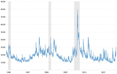
Besides the volatility smile, the S&P 500 volatility index in Figure 2.4.2 also shows that volatility is not constant across different timing. Figure 2.4.2 shows that the implied volatility

(34)

2.4. THE LIMITATIONS OF THE BSM 23

from 1990 to today stayed mostly below 30% with some occasional spikes. The biggest spike occurred during financial crisis in 2008. Even during some periods when the implied volatility was very low and stable, it was never constant.

Figure 2.4.2. the daily level of the CBOE VIX Volatility Index implied by S&P 500 back to 1990

2.4.2 Shortcomings of the stock log-normal distribution

The BSM assumes the lof of stock return is normally distributed, but in reality, the stock return distribution is not normally distributed. There is asymmetry and extreme outlier along x axis compared to the normal distribution, which reflects the stock return is not normally distributed. The degree of asymmetry and outlier can be measured by skewness and kurtosis separately in statistics.

We will first give the definition of normal distribution and log-normal variable in order to give the mathematical sense of what it means for the log of stock return to be normally distributed. We can view the stock return as x in the following definitions. After we introduce the log of stock return is normally distributed, we move into the definitions of skewness and kurtosis. We will discuss how skewness and kurtosis indicate the risk of stock investment. The definitions and the figures for this section are cited from [12],[13], [11],[15], and [10] .

(35)

24 2. THE BLACK-SCHOLES OPTION PRICING MODEL

Definition 2.4.1. A random variable x is normal or normally distributed with mean µ

and varianceσ2, if it is continuous with probability density function

f(x) = √1

2πσe

−(x−µ)2

2σ2 for all −∞< x <∞.

The distribution of such an x is called the normal distribution with mean µ and variance

σ2. 4

Definition 2.4.2. A variable xis a log-normal random variable with meanµand variance

σ2 if logX is a normal random variable with mean µ and variance σ2,which is defined by the formula

Y =ex withx being a normal random variable.

4

The purpose of introducing both Definition 2.4.2 and Definition 2.4.2 is to show that the fact that log of stock return (x) is normally distributed means that the stock return is log-normally distributed. But, in this project, we use the term– log-normal stock return to describe log of stock return is normally distributed.

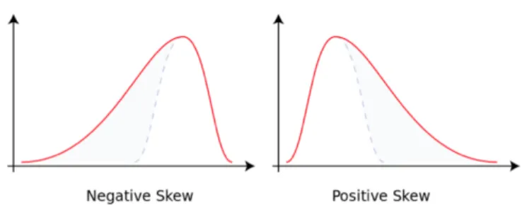
Definition 2.4.3. . Skewness is a measure of how asymmetric the data are. A distribution with a skewness of zero is perfectly symmetric. In comparison, a distribution with a negative skewness will have a longer tail on the left side than on the right side; the opposite is true of positive skewness, as it is shown in the Figure 2.4.3 cited from [11].

1. Right SkewedorPositive Skewedmeans the tail on the right side of the distribution is longer than the left side. A relatively high positive skewness indicates stock returns deep in the right tail of the distribution as described in [15]. This means that there is more chance for gain than loss. Thus having right skewed means the investment is less risky.

2. Left Skewed orNegative Skewed means the tail on the left side of the distribution is longer than the tail of the right side. A relatively high negative skewness indicates the big

(36)

2.4. THE LIMITATIONS OF THE BSM 25

downside moves, or loss of stock return are more likely than big upside moves, or gain. Thus having left skewed means the investments are more risky.

4

Figure 2.4.3. Skewness

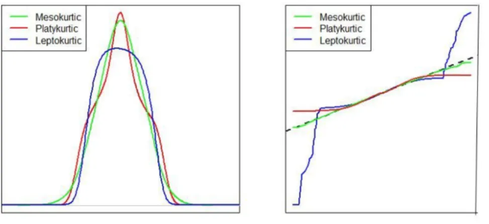
Definition 2.4.4. Kurtosis is a measure of whether the data are heavy-tailed or light-tailed relative to a normal distribution. That is, data sets with highkurtosistend to have heavy tails, or outliers. Data sets with lowkurtosis tend to have light tails, or lack of outliers. The figure 2.4.4 is cited from [13]. Kurtosis helps the investor gauge an asset’s level of risk.

There are three types of kurtosis depends on the kurtosis values, which are mesokurtic, leptokurticand platykurtic. Basically mesokurtic is the normal distribution(bell-curve). We will focus on leptokurtic and platykurtic, especially leptokurtic.

1. when kurtosis value is positive, it is called leptokurtic. It is a statistical distribution where there are extreme outliers or points alongx-axis, resulting in a higher kurtosis than found in a normal distribution.

For investors, having leptokurtic distribution for stock return means the investors will experience occasional large fluctuations more often than predicted by the normal distribu-tions. This is due to the extreme values, or outliers which gives more chance of losing or gaining suggested by the normal distribution.

2. when kurtosis value is negative, it is called platykurtic. It is a particular statistical distribution with thinner tails than a normal distribution. Because this distribution has thin tails, it has fewer outliers than mesokurtic and leptokurtic distributions.

(37)

26 2. THE BLACK-SCHOLES OPTION PRICING MODEL

For investors, having platykurtic distribution for the stock return means there are less extreme values than the normal distribution. This means the investment is less risky and stable and has less major fluctuations.

4

Figure 2.4.4. Kurtosis

Generally, the stock investors care more about the left skewed and the leptokurtic because having leptokurtic distribution indicates that there are higher chance of extreme values for stock return and higher chance of loss and gain, and having left skewed distribution indicates that big downsides moves are more likely than big upsides moves. We will use two figures to show that the BSM assumptions in log-normal stock return is not consistent with what is observed in the market.

Figure 2.4.5 cited from [18] is the frequency distribution of SPX log returns over 77-year period from 1928 to 2005. The x-axis is the continuously compounded stock return and the y-axis is the density. Notice that the x-axis has been extended to the left to accommodate the return. We can see that this distribution is not normally distributed; instead it is highly peaked and leptokurtic (fat-tail, outlier).

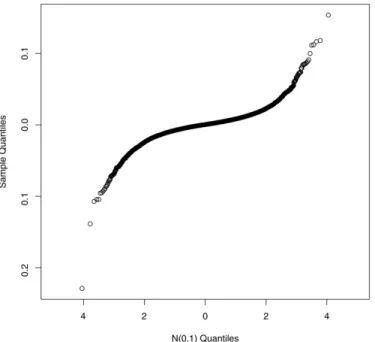
Figure 2.4.6 cited from [18] is the Q-Q plot, which shows how extreme the tails of the empirical distributions of returns are relative to the normal distribution. The plot would be a straight line

(38)

2.4. THE LIMITATIONS OF THE BSM 27

Figure 2.4.5. Frequency distribution of 77 yeas of SPX daily log-returns compared with the normal distribution.

of the empirical distribution were normal. We can see the long tail toward both sides and this is called leptokurtic as described in 2.4.4. Both Figure 2.4.5 and Figure 2.4.6 show that the BSM log-normal stock return assumption does not hold in the reality. There are usually high peak, fat tails observed in the market. As described in [18], the high peak and fat tails are the characteristics of mixture distribution with different variance. Thus it is necessary to move from the constant volatility assumption in the BSM to stochastic volatility.

Figure 2.4.6. Q-Q plot of SPX daily log returns compared with the normal distribution. Note the extreme tails.

(39)

28 2. THE BLACK-SCHOLES OPTION PRICING MODEL

2.4.3 Leverage Effect and Clustering Effect

The Leverage Effect is the negative correlation between the stock price and the volatility. This means when there are high drops in the stock price, the volatility increases; when there in an increase in the stock price, the volatility decreases. This makes sense intuitively because the investors usually react more, when there are negative stock returns; whereas the investors become more confident, when there are positive stock returns.

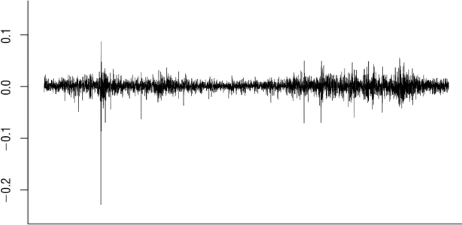
TheClustering Effectmeans the larger market moves are followed by large moves. While the smaller market moves are followed by small moves. This is the feature that cannot be captured by a model assuming a constant volatility. As we see in Figure 2.4.7, it is the log return of the SPX over a 15-year period. The x-axis is the time in years and the y-axis is log return of the SPX Index. We can see the volatility is actually auto-correlated, which means the volatility process might have some extreme cases but over the long-run it self-adjust to the mean value. See Figure 2.4.7. This tendency of toward the mean is a mean-reverting volatility process.

However, despite the fact that the limitations of the BSM, which shows the idealized assump-tions are not consistent with what is observed in the market, the BSM is still widely used. The main reason is its simple formula, which allows people to quickly estimate the option prices. It has become the benchmark among the option pricing models. But, it is still worth seeing how we can improve the BSM by changing its problematic assumptions, especially constant volatility to make the BSM more consistent to the reality. Thus in the next section, we will move from the constant volatility to stochastic volatility.

2.5

Moving to Stochastic Volatility

We have seen the constant volatility and the normally distributed stock return assumptions are not consistent with what is observed in the real market. The existence of volatility smile, the asymmetry and the fat tails show that the BSM leaves much room for improvement.

Many researches have done to improve its drawbacks and various models are proposed. One of the approach is to allow the volatility itself to be a random process. the Heston Model remains

(40)

2.5. MOVING TO STOCHASTIC VOLATILITY 29

Figure 2.4.7. SPX daily log-returns from December 31, 1984 to December 31, 2004. Note the -22.9% return om October 19, 1987.

the most popular one since its many advantages, which we will discuss in the details in the next chapter. Before moving into the Heston Model, it is important to understand the basic concept of the stochastic process. Remember that in the BSM, the stock price is assumed to be a stochastic process, but not the volatility. We will present the details of stochastic process in the following session.

2.5.1 Stochastic Process

This section is mainly cite from [20]. We will move from Wiener process to the generalized Wiener process. The understanding of this section will lay out the foundation for the Heston Model because the Heston Model involves two correlated Wiener process–one for the stock price and the other for the volatility. The appearance of the Winner process is where the randomness comes in the Heston Model.

Any variable whose value changes over time in an uncertain way is said to follow astochastic process.Stochastic processcan be classified as discrete time or continuous time. A discrete-time stochastic processis one where the value of the variable can change only at certain fixed points in time, whereas acontinuous-time stochastic processis one where changes can take place at any time.

(41)

30 2. THE BLACK-SCHOLES OPTION PRICING MODEL

A Markov process is a particular type of stochastic process where only the present value of a variable is relevant for predicting the future. The past history of the variable and the way that the present has emerged from the past are irrelevant.

The Brownian Motionsometimes also known as Wiener process is a particular type of Markov stochastic process. We consider a variable follow the Brownian Motion if it has the following two properties:

1. The change ∆z during a small period of time ∆ is

∆z=

√

∆t

where has a standardize normal distribution with mean 0 and standard deviation 1

N(0,1).

2. The value of ∆zfor any two different short intervals of time, ∆t, are independent. The value ∆zhas a normal distribution with mean of 0, standard deviation of√∆t, and variance of ∆t.

A generalize Wiener processfor a variablex is defined in terms ofdz as

dx=adt+bdz (2.5.1)

whereaand b are constants anddz is Wiener process.

The adt term implies that x has an expected drift rate of a per unit of time. The bdz term can be regarded as adding noise or variability to the path followed by x. The amount of this noise or variability isb timesdz (Wiener process).

A Wiener process has a standard deviation of 1. It follows thatb times a Wiener process has a standard deviation ofb. In a small time interval ∆t, the change ∆x in the value of x is given by

∆x=a∆t+b

√

∆t (2.5.2)

wherehas a standard normal distribution. It is shown that the change ofxin any time interval

(42)

2.5. MOVING TO STOCHASTIC VOLATILITY 31

generalized Wiener processgiven by Equation 2.5.1 has an expected drift rate( average drift rate per unit of time) ofaand a variance rate(variance per unit of time) of b2. It is illustrated in Figure 2.5.1.

(43)

(44)

3

The Heston Stochastic Volatility Model

Since the 1987 financial crisis, a number of models have been proposed to improve the BSM in order to reflect the market behaviors better than the BSM. The Heston Stochastic Volatility Model, for European option pricing, was developed by Steven Heston in 1993 to overcome the shortcomings of the BSM, especially the constant volatility assumption and the log-normal stock return assumption. It is one of the most popular stochastic volatility pricing models not only because it address the two major assumptions in the BSM by allowing the volatility itself to be a random variable, but also it takes the volatility smile, the leverage effect and the important mean-reverting property of volatility into account.

The Heston Model is based on nine input parameters, which are stock priceS, strike priceK, the risk-free interest rate r, maturity t, initial volatility V0, long-term volatility ¯V, the mean-reverting speed for volatilitya, and the correlation between stock price and volatilityρ. The first four input parameters are easily observable market data, which can be determined by looking at the market. The last five input parameters can be obtained using the calibration process which will be presented in the next chapter. The following sections are mainly cited from [24], [31], [17] and [29] .

(45)

34 3. THE HESTON STOCHASTIC VOLATILITY MODEL

3.1

the Heston Model

LetStbe the price of the underlying asset at timet,η be the volatility of the volatility process,

r be the risk-free interest rate,µ be the drift coefficients of the stock price, Vt be the variance at timet, ¯V be the long-term mean of variance,abe the rate of mean-reversion,dW_t1 anddW_t2

be two correlated Brownian motions andρ be the correlation coefficient.

Heston assumes the underlying asset S at time t with risk-free interest rate r follows the risk-neutral dynamics such that

dSt=µStdt+ p VtStdWt1 (3.1.1) dVt=a( ¯Vt−Vt)dt+η p VtdWt2 (3.1.2) dW_t1dW_t2 =ρdt (3.1.3) wherea, η, Vt>0.

Equation 3.1.1 shows that the stock price follows the stochastic process. Equation 3.1.2 shows that the volatility follows the stochastic process but also the volatility is toward the mean. Equation 3.1.3 shows that the two stochastic processes for both volatility and stock price are correlated. The details for each equation is presented in the following section.

3.1.1 Geometric Brownian Motion

Equation 3.1.1 is called geometric Brownian motion, which is the same assumption proposed in the BSM. This geometric Brownian motion can derived from viewing the generalized Wiener process in Equation 2.5.1 in terms of variable stock priceS and multiplyingS to the right side of the equation. By multiplying the stock price S on the right side means the stock price is proportional to its mean and to its standard deviation in the stochastic process. The µ is the expected rate of stock return and the √Vt is the volatility of the stock price.

√

VtdWt1 is the stochastic component of the return, or randomness component.

(46)

3.1. THE HESTON MODEL 35

3.1.2 Mean-Reverting Process

Besides keeping the same assumptions about stock price follows the stochastic process, Heston adds dVt = a( ¯Vt−Vt)dt+η

√

VtdWt2, which is a mean-reverting process also known as Cox-Ingersoll-Ross (CIR) process. This means the volatility tend to bounce toward its long-term mean.

This assumption is consistent with the behavior observed in financial market. If volatility were not mean-reverting, markets would be characterized by a considerable amount of assets with volatility exploding or going near zero. However, in practice, these cases are quite rare and generally short-lived as mentioned in [24].

The deterministic terma( ¯Vt−Vt) ensures the mean reversion of the volatility toward the long run value ¯Vt, with the speed of adjustment governed by the strictly positive parametera.

The standard deviation factorη√Vtavoids the possibility of negative volatility for all positive values ofη and θ, When the volatilityVt is close to zero, the standard deviationη

√

Vtbecomes very small, which dampens the effect of the random shock on the volatility. In other words, when the volatility gets close to 0, its evolution becomes dominated by the deterministic term, which pushes the volatility towards the long-term mean.

3.1.3 Correlated shocks between stock price and volatility

Heston introduces a correlated relationship between stock returns and volatility. This assumption allows modelling the statistical dependence between the stock return and and its volatility, which is a prominent feature of financial markets. In stock markets, volatility tends to increase when the stock price return decrease; whereas volatility tends to decrease when the stock price return increases. This is quite intuitive because investors usually react more, which drives the volatility to be higher, when there are high drops in the stock returns. Whereas when the stock return increases, investors become more confident which leads the volatility to be less .

The Heston Model provides a modeling framework that can take many of the specific char-acteristics that are typically observed in the behavior of financial market into account. But, its

(47)

36 3. THE HESTON STOCHASTIC VOLATILITY MODEL

advantages come at the expense of higher complicity. Compared to the BSM, the implementa-tion of the Heston Model requires more sophisticated mathematics and it takes more time to calculate the option price since it involves a challenging calibration to the market price in order to find the five missing parameters. We will explain the calibration later on.

3.2

Closed-Form Solution of the Heston Model

In this section, we follow the reasoning in Heston paper [4], but we cite the new formulation of Heston solutions from [24] and cite the pros and cons of the Heston Model from [?MRZEK]. Equa-tion 3.2.4, EquaEqua-tion 3.2.5, EquaEqua-tion 3.2.6, EquaEqua-tion 3.2.7, EquaEqua-tion 3.2.8 and EquaEqua-tion 3.2.9 are proposed by [24] who modifies the Heston characteristic function proposed by [18].

The present value of a European call option can be estimated using a probabilistic approach

C0 =S0Π1−e−rTKΠ2 (3.2.1)

,where the first term S0Π1 represents the present value of the underlying given an optimal exercise and the second terme−rTKΠ2 is the present value of the strike price of the strike price payment. Moreover, Π1 is the delta of the European call option and Π2 is the conditional risk neutral probability that the asset price will be greater thanK at the maturity. Both Π1 and Π2 represent the conditional probability of call option expiring in-the-money.

Provided that characteristic functionψHeston_{ln (}_S

t) (w) are known, the terms Π1 and Π2 are defined

via the Fourier transformation,

Π1 = 1 2+ 1 π Z ∞ 0 Re " eiwlnKψlnST(w−i) iwψlnST(−i) # dw (3.2.2) Π2 = 1 2+ 1 π Z ∞ 0 Re " eiwlnKψlnST(w−i) iw # dw (3.2.3)

Where Equation 3.2.2 and Equation 3.2.3 are smooth functions that decay rapidly and present no difficulties as mentioned in [4].

(48)

3.3. IMPLEMENTATION 37

Heston considers the characteristic function of these probabilities in the form

ψHeston_{ln (}_S_t₎ (w) =e

C(t,w)V+D(t,w)v0+iwlnS0ert

, (3.2.4)

and shows that

C(t, w) =a r ·t− 2 η2 ln 1−ge−ht 1−g (3.2.5) D(t, w) =r 1−e −ht 1−ge−ht, (3.2.6) where r±= β±h η2 ;h= p β2₋₄_αγ _(3.2.7) g= r r+ (3.2.8) α=−w 2 2 − iw 2 ;β =α−ρηiw;γ = η2 2. (3.2.9)

3.3

Implementation

1. Compute the Heston Characteristic Functionψ_{ln (}Heston_S

t) (w) in Equation 3.2.4

2. Substitute Heston Characteristic Function into Equation 3.2.2 and Equation 3.2.3 to com-pute Π1 and Π2.

3. After calculating probabilities Π1 and Π2, plug them back to Equation 3.2.1.

4. Equation 3.2.1 returns a European call option price under the Heston Model.

3.4

Influence of Parameters

The section including the figures are mainly cited from [31], [35] and [17]. There have been many empirical studies that show the stock return is not normally distributed. There are fat tails (leptokurtic) and asymmetry shown in the stock returns. It is also suggested that the correlation

(49)

38 3. THE HESTON STOCHASTIC VOLATILITY MODEL

between stock return is negative, which is called the leverage effect. There is also the volatility clustering effect observed in the market. Thus it is important to understand the meaning of the Heston parameters which takes those above phenomena into account. The following five parameters are generated through the calibration process, which we will introduce in the next chapter.

• Initial variance parameterV0

As mentioned in [17], changing the initial variance allows adjustment in the height of the smile curve rather than the shape. Increasing the initial volatility, √V0 moves the implied volatility smile upwards. See Figure 3.4.1.

Figure 3.4.1. The effect of changing the initial variance v=√V0

• Long term variance parameter ¯V

Changing the long-term variance ¯V has the similar effect as changing the initial varianceV0. See Figure 3.4.2. The θ in the Figure 3.4.2 is the ¯V here.

• Mean-reversion speed parameter a.

As mentioned in [17], the mean reversion speed can be viewed as the degree of volatility clus-tering. As mentioned before, volatility clustering can be observed in the market; it means that large moves are followed by large moves, while small moves are more likely followed by small

(50)

3.4. INFLUENCE OF PARAMETERS 39

Figure 3.4.2. The effect of changing the long-term variance ¯V which is denoted asθ

moves. The mean reversion controls the curvature of the curve. If there is a increase in the mean reversion parameter, it flattens the volatility smile. If there is a decrease in the mean reversion parameter, the effect is the opposite. See Figure 3.4.3. Thek in Figure 3.4.3 is theahere.

Figure 3.4.3. The effect of changing the mean reversion speedawhich is denoted ask in the figure

• The volatility of volatility parameterη

The parameter η controls the kurtosis (peak) of the underlying asset return distribution. When η is zero, the volatility becomes deterministic. In other words, the volatility is constant, so the distribution of stock price follows the normal distribution. Otherwise, asηincreases causes the kurtosis to increase,which creates the fat tails on the both sides. Note the higher η means the volatility is more volatile, which states that the market has a greater chance of extreme movements. See Figure 3.4.4. Theσ in the Figure 3.4.4 means the volatility of varianceη here.

(51)

40 3. THE HESTON STOCHASTIC VOLATILITY MODEL

Figure 3.4.4. The effect ofη which is denoted asσon the kurtosis of the density function

The parameterρis the correlation between the log-returns and volatility of the stock. It affects the skewness or asymmetry of the underlying asset return distribution. See Figure 3.4.5.

If ρ >0, the volatility will increase as the stock price increase. This will spread the right tail and squeeze the left tail of the distribution creating a long right-tailed distribution, which is called right skewed. See Figure 3.4.5, when ρ is 0.9, there is a right skewed.

If ρ < 0, the volatility will decrease while the stock price decrease.This will spread the left tail and squeeze the right tail of the distribution creating a long left-tailed distribution, which is called left skewed. See Figure 3.4.5, whenρ is -0.9, there is a left skewed.

If ρ= 0, there is no effect to the skewness of distribution. Thus, the distribution is normally distributed. See Figure 3.4.5, whenρ is 0, it is a normal distribution.

3.5

Advantages and Disadvantages of the Heston Model

Many researchers and scholars have studied the importance of the Heston, but this is still a model. In other words, this is a model which is used to estimate the market option price, but it is not a perfect model. This section summarize both the advantages and disadvantages of the Heston Model. We cite the information from [17] and [29].

(52)

3.5. ADVANTAGES AND DISADVANTAGES OF THE HESTON MODEL 41

Figure 3.4.5. The effect ofρon the skewness of the density function

The advantages of the Heston Model:

1. The closed-form solution allows the calibration.

2. Heston models takes into account the leverage effect (negative correlation of stock returns and implied volatility), and it permits the correlation between the stock price and the volatility to be changed.

3. The volatility is mean-reverting.

4. The form of the Heston Model used to model price dynamics allows for non-lognormal probability distribution.

The disadvantages of the Heston Model:

1. Since volatility is not easily observable in the market, the parameters values in the Heston Model are not easily estimated. The values depend on the algorithms being used in the calibration process.

2. The price produced by the Heston Model are quite parameter sensitive, thus the fitness of the model depends on the calibration. In other words, to have more realistic model