Working Paper No. 3 November 2007
Faculty of Management
Technology
W o r k i n g P a p e r S e r i e s
Ranking of Mutually Exclusive
Investment Projects
How Cash Flow Differences can
solve the Ranking Problem
by
Christian Kalhoefer
Faculty of Management Technology German University in Cairo
Al Tagamoa Al Khames 11835 New Cairo City – Egypt [email protected]
Ranking of Mutually Exclusive Investment Projects
How cash flow differences can solve the ranking problem
by
Christian Kalhoefer November 2007
Abstract
The discussion about the best method to be used in capital budgeting has been long and intensive. Differences between Net Present Value and Internal Rate of Return seem to cause everlasting problems, while especially the Internal Rate of Return often is neglected as an appropriate measure. A famous example of the problems caused by the different approaches is the ranking of mutually exclusive projects. The following paper is presenting an easy explanation, without introducing new and more complicated measures, but by simply explaining the nature of and differences between Net Present Value and Internal Rate of Return.
JEL classification
G31; G11
Keywords
Capital budgeting; internal rate of return; net present value; ranking problem; incremental approach; reinvestment rate
1.
Introduction
The ranking of mutually exclusive investment project is interesting for practice as well as in a theoretical point of view and has been broadly discussed since many years. The main concern is the potential difference between the assessment results derived from either Net Present Value (NPV) or Internal Rate of Return (IRR). These differences between Net Present Value and Internal Rate of Return seem to cause everlasting problems, while especially the Internal Rate of Return usually is neglected as an appropriate measure.
While several attempts have been made to deal with this problem, it seems as if previous solu-tions didn’t come to the core of the problem. Proposed suggessolu-tions usually either try to solve the problem by finding a new “interpretation” of the IRR or by creating highly sophisticated mathematical add-ons for or modifications of the IRR in order to get the same ranking infor-mation as the NPV.
From a mathematical point of view, the reasons for the different results are the cash flow dif-ferences between different investment projects. The major question when applying investment appraisal techniques to rank mutually exclusive projects is how to deal with these differences. This paper is presenting an explanation for these ranking differences, without introducing new and more complicated measures, but by analyzing the nature of and differences between Net Present Value and Internal Rate of Return. The aim of this paper is to explain how a correct usage of both investment appraisals leads to identical results, and it should clearly be men-tioned these results should not be misunderstood as a pleading to use the IRR as investment appraisal tool. The weaknesses of the IRR are still valid, but the ranking differences are ex-ceptional not a weakness the IRR can be blamed for.
Applying this approach, it will be shown that there are no different results between the two methods if they are applied correctly. In addition, the common explanation of different “rein-vestment assumptions” of the two methods will be confuted. Furthermore, the superiority of the Net Present Value approach will be confirmed.
2.
The Ranking Problem in Capital Budgeting
The most important and broadly used approaches in capital budgeting are the Net Present Value (NPV) and the Internal Rate of Return (IRR) (Tang and Tang 2003, Graham and Har-vey 2001, Drury and Tayles 1997, Bacon 1977).
The NPV is the sum of the discounted cash flows of the project.
( )
∑
= − + ⋅ = n 0 t t t 1 i CF NPV (1)where NPV = Net Present Value t = time index
n = end of maturity CFt = cash flow at t
i = interest rate
An investment should be accepted if the NPV is exceeding zero. Therefore, the interest rate used to discount the cash flows is the hurdle rate for the decision.
The IRR is the interest rate that, when applied to the NPV formula, gives a NPV of zero. In other words, it is the interest rate where the sum of the discounted cash flows equals the initial investment (Crean 2005, 324, Schuck 1995, 40).
( )
∑
= − + ⋅ = = n 0 t t t 1 r CF NPV 0 (2)where r = internal rate of return
The IRR shows the effective return of the internally invested capital. An investment should be undertaken if the IRR exceeds the applied interest rate i, because in this case it will have a positive net present value (Shapiro 2005, 22). Therefore, for the appraisal of a single invest-ment, both measures are equivalent: if the NPV of a cash flow is positive, the IRR will also exceed the interest rate i. It should be mentioned that the previous statement should not be misunderstood as a recommendation to use the IRR for investment decisions, as the problems of the IRR are well known, especially
(1) in some special cases the mentioned equality between IRR and NPV might not be true, and
(2) the IRR can only be used if a reasonable rate of return can be calculated. Due to the nature of the IRR as a root of a polynomial, in case of some special cash flow patterns this may not be possible (Brown 2006, 195).
Although these problems are well known, it seems as if decision makers still prefer the IRR over the NPV, maybe because it is easier or more common to understand and communicate. While the technical problems (see e.g. Brown 2006 for a summary) as well as differences
3
between NPV and IRR when judging a single project occur only in special cases, the IRR is probably still an accepted invested appraisal measure. The usage of the IRR is significantly more error-prone if the investor has to decide between mutually exclusive investment pro-jects. Therefore, in the following the focus will not be on the technical problems with IRR, but on the well know ranking problem. In this case, different ranking results are possible while using the two approaches. Therefore, the recommendation of which project to choose is not clear. Reasons and consequences have been broadly discussed, and several proposals have been made to overcome these inconsistencies. The solutions often create more complicated measures that should be used in addition or alternatively to the IRR (e.g. Crean 2005, Barney and Danielson 2004, Lefly 2003) or attempt to give a different interpretation of the measures (Tang and Tang 2003). This paper will show that all this is not necessary if both measures are applied correctly.
One of the main arguments used to explain the different results is called reinvestment assump-tion. It states the – generally correct – finding that differences between intermediate cash flows have to be recognized. The specific argument is that this is done through an assumption about their reinvestment rate and a broad discussion about this topic started in the 1950ies (e.g. Solomon 1956, Bierman and Smidt 1957) and is still ongoing. For the discussed invest-ment appraisal techniques the common understanding is that the NPV assumes a reinvestinvest-ment of intermediate cash flows at the cost of capital while in case of the IRR the cash flow rein-vestment rate equals the IRR (Shapiro 2005, 26, Van Horne and Wachowicz 2005, 329, Pogue 2004, 40, Lefley 2003, 18). Although the reinvestment argument is common to explain different results between IRR and NPV, it is based on a wrong interpretation. To begin with a mathematical analysis of the formulas presented above, it can be seen that no reinvestment assumption is necessary to calculate NPV and IRR (Dudley 1972, 907). Therefore, the reason for the different results is something else, namely an inconsequent application of the two methods: if the investment projects have different cash flow patterns, both of them are not directly comparable, at least not by an undifferentiated application of the investment apprais-als, because this may lead to a misinterpretation of the results. Instead, to make a proper deci-sion between mutually exclusive projects, an investor has to consider what will happen to the cash flow differences in between. Differences may exist in the initial investment, timing and amount of the following cash flows, and the maturity of the projects (Van Horne and Wa-chowicz 2005, 326).
If, for example, two mutually exclusive investment projects have to be compared, the first one with an initial investment of $ 100,000 and the second with an initial investment of $ 90,000, the investor must consider what happens to the $ 10,000 difference. This is of course true for all cash flow differences over the time. It is possible that the investment project originally being rejected becomes the superior one if these cash flow differences are recognized in an appropriate way.
The comparison of different cash flow patterns (CFP) by their differences is known as incre-mental approach (Hajdasinski 2004, Hajdasinski 1997, Fisher 1930), but the implications of this approach have not been stressed enough in the earlier literature. The usability of this ap-proach will be shown in the following sections. It will be clarified that no additional assump-tions or measures are necessary if investors fully understand the statements of NPV and IRR. It will also be pointed out, that, if applied and interpreted properly, both measures do not de-liver different ranking information.
3.
Explicit Handling of Cash Flow Differences – the Special Case
Assuming two investment projects A and B, the differences between the cash flow patterns can be mathematical described by A – B, or B – A respectively. In German literature, the re-sulting cash flow pattern is usually named “difference investment”, abbreviated DI. There-fore, the cash flow pattern of the DI can be calculated as follows:
A B DI CF CF
CF = − (3)
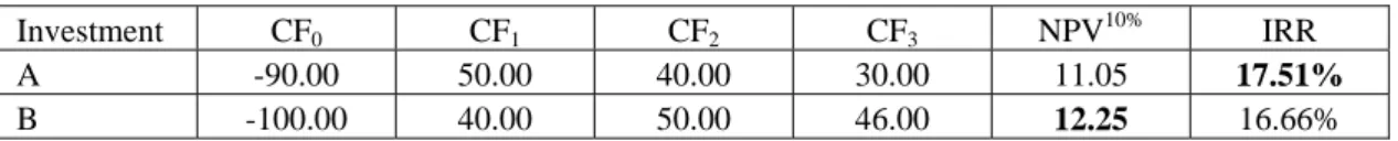
The investor must take into consideration what is going to happen to this difference ment. To explain the ranking problem with mutually exclusive projects, assume two invest-ment projects A and B, both with a CFP showing one initial cash outflow, followed by several cash inflows. This assumption assures that no mathematical problems occur while calculating the IRR. As usual, all cash flows are accumulated at yearend. Furthermore, the initial cash outflow of A is assumed to be smaller than the one B; and the calculation of NPV and IRR will result in a higher NPV for B, while the IRR of A is higher. Recommendation is to choose B if the investor is referring to NPV, or to choose A if the investor refers to the IRR. There-fore, the decision which investment to choose is not clear. The following Table 1 shows a numerical example that fits to this description. The NPV has been calculated at i = 10%.
5
Investment CF0 CF1 CF2 CF3 NPV10% IRR
A -90.00 50.00 40.00 30.00 11.05 17.51%
B -100.00 40.00 50.00 46.00 12.25 16.66%
Table 1: Exemplary data for mutually exclusive investment projects
As investment A is reporting the lower NPV, including the DI into the considerations might result in A plus the DI giving a higher NPV than B. With reference to the above description, the DI can be calculated as B – A. With the assumption about the initial investments (A being less expensive than B), their difference (CF0DI) will be negative. This simply stresses the
in-terpretation of a difference investment as a cash flow pattern starting with a cash outflow; however, this is not a necessary condition for the following arguments.
Investment CF0 CF1 CF2 CF3
A -90.00 50.00 40.00 30.00
B -100.00 40.00 50.00 46.00
DI = B – A -10 -10 10 16
Table 2: Derivation of the difference investment
The DI cash flow represents either an investment (if negative) or a credit taken (if positive). Therefore, the cash flows will have financial effects in later years, where either an investment will give some return or a credit has to be paid back. It is assumed that both alternatives are constructed as zero coupon bonds with a certain interest rate z. The financial effects of the DI are included in the calculation by compounding the relevant DI cash flows with the interest rate z to the last year. The results are shown in Table 3.
t / In-vestment cash flow 0 1 ... n A A 0 CF CF 1A ... A n CF B B 0 CF CF 1B ... CF nB DI A 0 B 0 DI 0 CF CF CF = − CF1DI =CF1B −CF1A ... CFnDI =CFnB −CFnA A + DI B 0 A 0 B 0 A 0 DI 0 A 0 CF CF CF CF CF CF = − + = + B 1 A 1 B 1 A 1 DI 1 A 1 CF CF CF CF CF CF = − + = + ...
(
)
(
)
∑
∑
= − = − + ⋅ − + = + ⋅ − + + n 0 t t n DI t B n n 0 t t n DI t DI n A n z 1 CF CF z 1 CF CF CFIncluding the DI leads to identical cash flows of B and (A + DI) for all t < n. In the last year, the cash flow of (A + DI) equals the cash flow of B plus the sum of the compounded cash flows of DI.
A note should be made concerning the algebraic sign of the compounded DI cash flows in t = n. It must be stated as minus, because if the original DI cash flow has been negative (repre-senting an investment), the latter one must be positive (repre(repre-senting the positive return of the investment). In case of an originally positive DI cash flow (representing a credit taken by the investor), the last year’s cash flow must be negative to indicate the payback of the credit. An important result of the previous considerations is that – as all cash flows for t < n are iden-tical – both investment alternatives can be compared simply by comparing the last year’s cash flows. The project with the higher cash flow will be selected. This result highlights the impor-tance of the DI, because the cash flow in t = n is dependent on the interest rate z used to com-pound the DI cash flows. To get an idea about this rate of return, it will be interesting to in-vestigate the rate where both investments are equal. Apparently, this will be the case if the future value (FV), expressed as sum of the compounded DI cash flows, equals zero, because in this case CFnA + CFnDI + 0 = CFnB. To fulfill this requirement, z must be the IRR of the DI
cash flow. This special interest rate is called Fisher’s rate of intersection f (Van Horne and Wachowicz 2005, 328). The following formula shows this effect mathematically.
(
)
∑
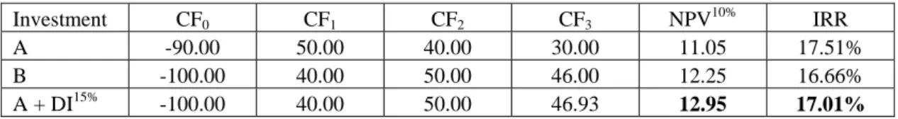
= − = + ⋅ − = n 0 t t n DI t DI n CF 1 f 0 FV (4)In the example, f is 13.20%. The knowledge of f has an important consequence: as soon as z is exceeding f, the combination of A and DI will result in a higher last year’s cash flow; there-fore the combination of A and DI will be superior to B. The exemplary calculation in Table 4 uses z = 15%. As 15% exceeds 13.20%, the combination of A and DI is better than B, a fact that can easily be recognized by a comparison of the two cash flow patterns. They are identi-cal except for the third year, where the cash flow of (A + DI) is higher than the one of B.
Investment CF0 CF1 CF2 CF3 NPV10% IRR
A -90.00 50.00 40.00 30.00 11.05 17.51% B -100.00 40.00 50.00 46.00 12.25 16.66% A + DI15% -100.00 40.00 50.00 46.93 12.95 17.01%
Table 4: Exemplary calculation of A and DI with z = 15%
It should be mentioned that, up to this point, none of the typical investment appraisal tech-nique is necessary to get this result. It is nothing but a simple comparison of cash flows.
Ap-7
parently, if the investor evaluates the two described cash flows B and (A + DI), B will have the lower NPV and the lower IRR. These ratios are shown in Table 4 for the example, where both measures are higher for the combination of A and DI. There is no discrepancy between NPV and IRR. With respect to this clear finding, different appraisal results offered by NPV and IRR are even more astonishing. The reason will be explained in the last chapter.
4.
Explanation of Ranking Differences – the Common
Application of Investment Appraisals
The previous analysis has shown that any investor explicitly knowing or assuming an invest-ment rate z and properly applying it to the DI as described above will not face the problem of different results with NPV and IRR. The investment rate z can also directly be used to find the better alternative: if z is exceeding f, the investor should choose the project with the lower NPV together with the DI, as the combination of both will have a higher NPV (and IRR!) than the alternative project. But to assume an appropriate z might be difficult or impossible for an investor and it is not the purpose of this paper to enter the discussion about the determination of an appropriate rate (see e.g. Meyer 1979). Therefore, the next step will be to analyze the situation without an explicit assumption. This analysis is especially important as it considers the typical application of NPV and IRR, i.e. investors usually don’t assume an explicit z when working with NPV and IRR.
Generally speaking, as long as the investor doesn’t assume an explicit rate of return for the DI, the simple application of NPV and IRR calculation will result in an implicit assumption, while the problem is that these assumptions differ between the two methods. In other words: the mathematical interpretation of NPV and IRR is true only if z is applied in a specific way. It should be mentioned again that the investment rate z is not the commonly discussed rein-vestment rate for intermediate cash flows, but only necessary for the difference inrein-vestment within the ranking decision.
To understand the mathematical consequences of the implicit assumptions, it has to be proven under which circumstances NPV and IRR deliver the correct mathematical result when in-cluding the DI. Starting with the NPV, without an explicit assumption of z the result of the calculation of the NPV is correct only if z = i. Applying this to the previously explained for-mula, the FV of the DI can be written like
(
)
( )
⎥ ⎦ ⎤ ⎢ ⎣ ⎡ − − ⋅ + =∑
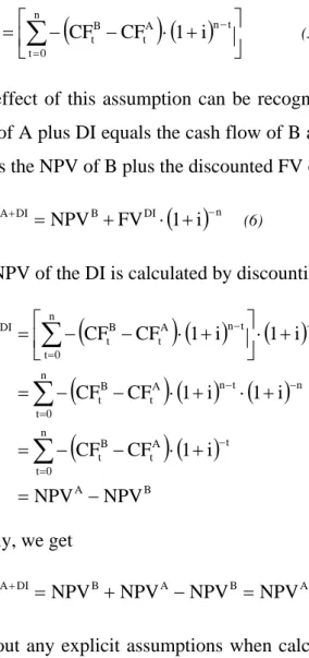
= − n 0 t t n A t B t DI n CF CF 1 i FV (5)The effect of this assumption can be recognized by calculating the NPV again. As the cash flow of A plus DI equals the cash flow of B at any time except for t = n, the NPV of (A + DI) equals the NPV of B plus the discounted FV of the DI.
( )
n DI B DI A i 1 FV NPV NPV + = + ⋅ + − (6)The NPV of the DI is calculated by discounting the Future Value as shown in equation (5).
(
)
( )
( )
(
)
( ) ( )
(
)
( )
B A n 0 t t A t B t n n 0 t t n A t B t n n 0 t t n A t B t DI NPV NPV i 1 CF CF i 1 i 1 CF CF i 1 i 1 CF CF NPV − = + ⋅ − − = + ⋅ + ⋅ − − = + ⋅ ⎥ ⎦ ⎤ ⎢ ⎣ ⎡ + ⋅ − − =∑
∑
∑
= − − = − − = − Finally, we get A B A B DI A NPV NPV NPV NPV NPV + = + − = (7)Without any explicit assumptions when calculating the NPV to compare different cash flow patterns, implicitly a rate of return of i is assumed for the difference investment (again: not for a reinvestment of the cash flows themselves!), because otherwise the calculated result would not be correct. As a result, it can be seen that a ranking decision based on the NPV will be correct, because an investment rate of i for the DI doesn’t change the calculated NPV.
The following Table 5 shows the results for the previous example. Again, both investment appraisals will result in the same ranking if applied correctly, i.e. on the complete cash flow.
Investment CF0 CF1 CF2 CF3 NPV10% IRR
A -90.00 50.00 40.00 30.00 11.05 17.51% B -100.00 40.00 50.00 46.00 12.25 16.66%
A + DI10% -100.00 40.00 50.00 44.41 11.05 16.06%
Table 5: Results of the implicit assumption of the NPV
The assumption of z = i matches the common prerequisite of a perfect capital market. There-fore, an investor not willing or not able to assume a reasonable investment rate z is doing fine with the application of the NPV as an appraisal technique. It can be seen that the correct
ap-9
plication will lead to a lower IRR for the alternative with the lower NPV, so there are no dif-ferent signals between the two methods.
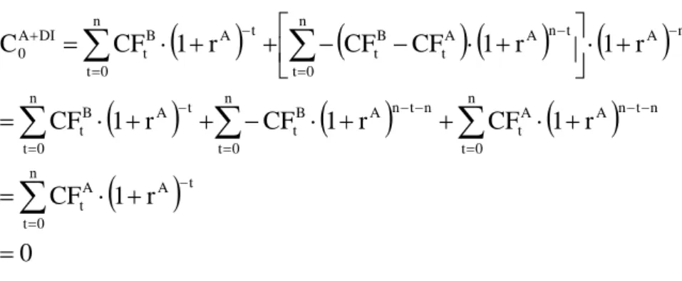
For the IRR, the explanation is quite similar. The mathematical information of the IRR, ap-plied to the total cash flow (project and DI) is correct only if the investment rate z equals the IRR of the project. The following equation describes this effect for the combination of A and DI.
(
)
(
) (
) (
)
(
)
(
)
(
)
(
)
0 r 1 CF r 1 CF r 1 CF r 1 CF r 1 r 1 CF CF r 1 CF C t A n 0 t A t n t n A n 0 t A t n t n A n 0 t B t n 0 t t A B t n A n 0 t t n A A t B t n 0 t t A B t DI A 0 = + ⋅ = + ⋅ + + ⋅ − + + ⋅ = + ⋅ ⎥ ⎦ ⎤ ⎢ ⎣ ⎡ − − ⋅ + + + ⋅ = − = − − = − − = = − − = − = − +∑
∑
∑
∑
∑
∑
The equation shows that the result of the discounting can be zero only if the IRR of A is used as z. Therefore, it is obvious that the investment with the higher IRR has to be preferred, as the same higher IRR will be applied for the DI. But as before, applying the NPV on the com-plete cash flow will give the same ranking as the IRR, so the correct application of both NPV and IRR will lead to the same results. Correct means using the complete cash flow, i.e. includ-ing the DI. The application of these findinclud-ings on the example data can be seen in Table 6.
Investment CF0 CF1 CF2 CF3 NPV10% IRR
A -90.00 50.00 40.00 30.00 11.05 17.51% B -100.00 40.00 50.00 46.00 12.25 16.66% A + DI17.51% -100.00 40.00 50.00 48.29 13.96 17.51%
Table 6: Results of the implicit assumptions of IRR
Although the NPV/IRR discrepancy might be solved by the correct interpretation of the num-bers, the application of the IRR method still owns it’s broadly discussed problems. Within the ranking problem, the most crucial fact is, as several different cash flows usually lead to sev-eral different IRRs, consequently sevsev-eral different investment rates z are applied to judge in-vestment projects. This is not rational, because as a result the return of the DI would be di-rectly dependent on the original cash flow. Furthermore, the return of future investment op-portunities will usually not be related with today’s investment projects’ IRR. In addition, the application of an interest rate other than i for the difference investment doesn’t follow the assumptions of a perfect capital market. Therefore, if the investor is not able or willing to
se-lect an appropriate rate of return for the difference investment, it is still recommended to use the NPV for investment decisions.
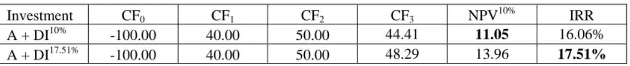
To summarize the analysis for the exemplary data, both relevant cash flows for investment A are mentioned in Table 7. It can again be recognized that the original mathematical results of NPV and IRR (see Table 1) are derived from different assumptions regarding the cash flows, which is the reason for the different ranking recommendation when compared to investment B.
Investment CF0 CF1 CF2 CF3 NPV10% IRR
A + DI10% -100.00 40.00 50.00 44.41 11.05 16.06% A + DI17.51% -100.00 40.00 50.00 48.29 13.96 17.51%
Table 7: Comparison between NPV and IRR cash flows
From the previous analysis the reason for different results between IRR and NPV in the rank-ing problem is easy to address. Without an explicit assumption the mathematical results of both appraisals are correct only if specific interest rates are assumed for the DI: i for the NPV and r for the IRR. These different interest rates lead to different cash flows, so at the end both techniques will not assess identical cash flows. Apparently, under these conditions the results can be different. The problem can obviously be avoided if both appraisals are applied to iden-tical cash flows as described in this paper.
5.
Conclusion
The broadly discussed ranking problem is a result of an insufficient application of the invest-ment appraisal techniques. For mathematical reasons, the results of the calculations are cor-rect only if certain assumptions are made concerning the investment rate for the difference investment. As these assumptions are not identical, both methods will finally assess different cash flows. Therefore, the results can be different. To avoid this problem, both investment appraisal techniques should be applied on identical cash flows. In this case, different rankings are not longer existent. These findings of course do not prevent the investor to make a deci-sion concerning the difference investment. As long as he is not able or willing to choose an appropriate explicit rate of return for the difference investment, he will still have to choose between net present value and internal rate of return. Although the ranking problem can be avoided when applying the methods correctly, as the assumption concerning z when applying IRR is questionable and the other well-known problems of the IRR still exist, the usage of the
11
NPV is recommended if no explicit choice for the return of the difference investment can be made.
References
Bacon, P.W. (1977): The Evaluation of Mutually Exclusive Investments. Financial Manage-ment, 6, No. 2: 55 – 58
Barney, L.D. Jr. and Danielson, M.G. (2004): Ranking Mutually Exclusive Projects: The Role of Duration. The Engineering Economist 49: 43 – 61
Bierman, H. and Smidt S. (1957): Capital Budgeting and the Problem of Reinvesting Cash Proceeds, The Journal of Business, 30, No. 4: 276 – 279.
Brown, R.J. (2006): Sins of the IRR, Journal of Real Estate Portfolio Management 12: 195 – 199
Copeland, T.E., Weston, J.F., and Shastri, K. (2005): Financial Theory and Corporate Policy, Fourth International Edition, Boston et al.
Crean, M.J. (2005): Revealing the True Meaning of the IRR via Profiling the IRR and Defin-ing the ERR, Journal of Real Estate Portfolio Management, 11: 323 – 330
Drury, C. and Tayles, M. (1997): The misapplication of capital investment appraisal tech-niques, Management Decision, 35/2: 86 – 93
Dudley, C.L. Jr. (1972): A Note on Reinvestment Assumptions in Choosing between Net Pre-sent Value and Internal Rate of Return, The Journal of Finance, 27, No. 4: 907 – 915. Fisher, I. (1930): The Theory of Interest, Macmillan
Graham, J.R. and Harvey, C.R. (2001): The theory and practice of corporate finance: Evi-dence from the field, Journal of Financial Economics, 60: 187 – 243
Hajdasinski, M.M. (1997): Technical Note – Comments on “Using Heuristics to Evaluate Projects: The Case of Ranking Projects by IRR”, The Engineering Economist, 42: 163 – 166
Hajdasinski, M.M. (2004): Technical Note – The Internal Rate of Return (IRR) as a Financial Indicator, The Engineering Economist, 49: 185 – 197
Meyer, R.L. (1979): A Note on Capital Budgeting Techniques and the Reinvestment Rate,
The Journal of Finance, 34, No. 5: 1251 – 1254.
Pogue, M. (2004): Investment appraisal: a new approach. Managerial Auditing Journal, 19: 565 – 570
Schuck, E. (1995): Reinvestment rate risk analysis: a comment. Journal of Property Evalua-tion and Investment, 13: 39 – 50
Shapiro, A.C. (2005): Capital Budgeting and Investment Analysis, Upper Saddle River Solomon, E. (1956): The Arithmetic of Capital budgeting Decisions, Journal of Business
XXIX, No. 2: 124 – 129.
Tang, S.L. and Tang H.J. (2003): Technical Note: The Variable Financial Indicator IRR and the Constant Economic Indicator NPV. The Engineering Economist 48: 69 – 78
Van Horne, J.C. and Wachowicz, J.M. jr. (2005): Fundamentals of Financial Management, twelfth edition, Harlow et al.