!
Università degli studi di Trieste
XXVII CICLO DEL DOTTORATO DI RICERCA IN ASSICURAZIONE E FINANZA: MATEMATICA E GESTIONE
PRICING THE GUARANTEED LIFETIME
WITHDRAWAL BENEFIT (GLWB) IN A
VARIABLE ANNUITY CONTRACT
(Settore scientifico-disciplinare: SECS-S/06)
Dottoranda
MARIANGELA SCORRANO Coordinatore
PROF. GIANNI BOSI Supervisore di tesi
PROF.SSA ANNA RITA BACINELLO Co-Supervisore di tesi
DOTT. MASSIMILIANO KAUCIC
Contents
Introduction v
1 Variable Annuity products 1
1.1 Introduction to annuities . . . 1
1.2 History and development of the Annuity market . . . 6
1.3 Variable annuity products: the GMxB features . . . 8
1.4 Risks underlying Variable Annuities . . . 21
1.5 Variable annuities during the recent market Crisis . . . 26
1.6 Variable annuities around the world . . . 30
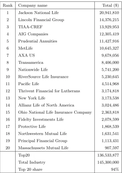
1.6.1 U.S.A . . . 30
1.6.2 Japan . . . 36
1.6.3 Europe . . . 41
1.7 A brief literature review . . . 44
2 The GLWB option: the valuation model 47 2.1 The structure of the contract . . . 47
2.2 The valuation model . . . 50
2.2.1 The financial market . . . 51
2.2.2 The mortality model . . . 56
2.2.3 The combined model . . . 60
3 The deterministic model: numerical results 67
3.1 Numerical results . . . 67
4 Generalization of the pricing model: stochastic interest rate 83 4.1 Stochastic interest rates models . . . 83
4.2 The CIR model . . . 85
4.3 Numerical results . . . 87
5 Generalization of the pricing model: stochastic volatility 97 5.1 Stochastic volatility models . . . 98
5.2 Numerical results . . . 100
6 The multi-factor model 107 6.1 Multi-factor models . . . 107
6.2 Heston-CIR hybrid pricing model . . . 107
7 Conclusion 115 A An introduction to Stochastic Calculus 117 A.1 Preliminary notions . . . 117
A.2 Stochastic Processes . . . 119
A.2.1 The Wiener process . . . 121
A.3 Stochastic Differential Equations . . . 122
A.4 Numerical approaches to SDEs . . . 124
A.4.1 Time discrete approximations . . . 125
A.4.2 Convergence of SDE solvers . . . 127
Acknowledgements
This thesis has been submitted to the University of Trieste in fulfillment of the re-quirements for the Doctoral degree in “Insurance and Finance: Mathemathics and Management” at the Department of Economics, Business, Mathematical and Statisti-cal Sciences “Bruno De Finetti”. I want to start expressing a sincere acknowledgement to my supervisors Prof.ssa Anna Rita Bacinello and Dott. Massimiliano Kaucic, for their guidance and encouragement. Special thanks go to Prof. Gianni Bosi, and to his predecessor, Prof. Vicig Paolo, who provided me with the opportunity to embark on this journey. Finally, a special thanks to my parents for their support, patience and love, for giving me the possibility to study.
Introduction
The purpose of life insurance is to provide financial security to policyholders and their families. Traditionally, this security has been guaranteed through a lump sum payable according to the death or survival of the insured. Against the payment of one or more premiums for the duration of the contract, the policyholder was enti-tled to the insured sum. These annuities used to provide policyholders with a good return in bull markets, since the guaranteed amount was determined by the policy-holder’s age and the level of interest rates. However, in the last decades, as interest rates declined, these contracts became less appealing. Insurance markets around the world have begun to change. Increasing life expectancy, as well as reduction of state retirement pensions in several countries have led to the rapid growth of new needs among consumers, and to the subsequent introduction of new products. The public has become more aware of investment opportunities outside the insurance sector and is increasingly trying to seize all the benefits of equity investment in conjunction with mortality protection. Over the last years, the competition with alternative invest-ment vehicles offered by the financial industry has generated substantial innovation in the design of life products and in the range of provided benefits. In particular, equity-linked policies have become ever more popular, exposing policyholders to fi-nancial markets and providing them with different ways to consolidate investment performance over time as well as protection against mortality-related risks.
Interesting examples of such contracts are variable annuities. First introduced in 1952 in the United States, this kind of policy experienced remarkable growth in Europe, especially during the last decade, characterized bybearish financial markets
and relatively low interest rates. The success of these contracts is due to the presence of tax incentives, but mainly to the possibility of underwriting several rider benefits that provide protection of the policyholder’s savings for the period before and after retirement. These forms of guarantees fall in two main categories: living benefits and death benefits. In particular, the provision of more and more attractive living benefits, in order to meet consumers’ new needs, has been an important factor in the success of variable annuities.
In this thesis, we focus on the Guaranteed Lifetime Withdrawal Benefit (GLWB) rider. This option offers the security of guaranteed capital and covers the longevity risk, while providing flexible payout options. Moreover, it enables policyholders to take advantage of continuous participation in the value appreciation of the fund in-vestments (by means of “ratchet” mechanisms, which link the increase of the account value with the one in the guaranteed amounts). For the affluent baby-boomers who are now approaching retirement, such variable annuities have been particularly ap-pealing as protection against market and longevity risks, when making the transition from the accumulation to the decumulation phase.
In this thesis, we propose a valuation model for the policy using tractable financial and stochastic mortality processes in a continuous time framework. We analyze the policy considering two points of view, the policyholder’s and the insurer’s, and assum-ing a static approach, in which policyholders each year withdraw just the guaranteed amount. In particular, we have based ourselves on the model proposed in the paper
“Systematic mortality risk: an analysis of guaranteed lifetime withdrawal benefits in
variable annuities” by M. C. Fung, K. Ignatieva and M. Sherris (2014), with the
aim of generalizing it later on. The valuation, indeed, is performed in a Black and Scholes economy: the sub-account value is assumed to follow a geometric Brownian motion, thus with a constant volatility, and the term structure of interest rates is assumed to be constant. These hypotheses, however, do not find justification in the financial markets. In order to consider a model better reflecting the market, we seek to weaken these misspecifications with the introduction of a stochastic process for the term structure of interest rates and for the volatility of the underlying account. We
address these two hypotheses separately at first, and then afterwards. As part of our analysis, we implement the theoretical model using a Monte Carlo approach. To this end, we have created ad hoc codes based on the programming language MATLAB, exploiting its fast matrix-computation facilities.
The work is organized as follows.
Chapter 1. This chapter has an introductory purpose and aims at presenting the
basic structures of annuities in general and of variable annuities in particular. We offer an historical review of the development of the VA contracts and describe the embedded guarantees. We examine the main life insurance markets in order to high-light the international developments of VAs and their growth potential. In the last part we retrace the main academic contributions on the topic.
Chapter 2. Among the embedded guarantees, we focus in particular on the
Guaran-teed Lifetime Withdrawal Benefit (GLWB) rider. We analyze a valuation model for the policy basing ourselves on the one proposed by M. Sherris (2014). We introduce the two components of the model: the financial market, on the one hand, and the mortality intensity on the other. We first describe them separately, and subsequently we combine them into the insurance market model. In the second part of the chapter we describe the valuation formula considering the GLWB from two perspectives, the policyholder’s and the insurer’s.
Chapter 3. Here we implement the theoretical model creating ad hoc codes with the
programming language MATLAB. Our numerical experiments use a Monte Carlo ap-proach: random variables have been simulated by MATLAB high level random num-ber generator, whereas concerning the approximation of expected values, scenario-based averages have been evaluated by exploiting MATLAB fast matrix-computation facilities. Sensitivity analyses are conducted in order to investigate the relation be-tween the fair fee rate and important financial and demographic factors.
Chapter 4. The assumption of deterministic interest rates, which can be
accept-able for short-term options, is not realistic for medium or long-term contracts such as life insurance products. GLWB contracts are investment vehicles with a long-term horizon and, as such, they are very sensitive to interest rate movements, which are
uncertain by nature. A stochastic modeling of the term structure is thus appropriate. In this chapter, therefore, we propose a generalization of the deterministic model al-lowing interest rates to vary randomly. A Cox-Ingersoll-Ross model is introduced. Sensitivity analyses have been conducted.
Chapter 5. Empirical studies of stock price returns show that volatility exhibits
“random” characteristics. Consequently, the hypothesis of a constant volatility is rather “counterfactual”. In order to consider a more realistic model, we introduce the stochastic Heston process for the volatility. Sensitivity analyses have been con-ducted.
Chapter 6. In this chapter we price the GLWB option considering a stochastic
pro-cess for both the interest rate and the volatility. We present a numerical comparison with the deterministic model.
Chapter 7. Conclusions are drawn.
Appendix. This section presents a quick survey of the most fundamental
con-cepts from stochastic calculus that are needed to proceed with the description of the GLWB’s valuation model.
Chapter 1
Variable Annuity products
1.1
Introduction to annuities
Among all the hurdles that investors face when saving for retirement, the most challenging is perhaps the risk of running out of money before they die.
Analyses show that the years just before and after retirement are a critical phase for the savings accumulated by investors throughout their working life. Traditional asset investments and the consequent sustainable retirement income streams are very sensitive to market fluctuations; a downturn in the markets could reduce savings to a level that will not provide sufficient revenue, and there may be not enough time for investors to recover their losses. Another remarkable source of uncertainty is the survival threshold. The fact that a retiree doesn’t know his/her date of death makes it harder to choose a consumption profile. Indeed, if he/she consumes relatively little in the first few years of retirement, he/she will make adequate provisions for a very long life. There is a chance, however, that he/she will die with a large sum of remaining capital. Alternatively, if the individual consumes excessively in the short term, he/she might need to reduce consumption later if he/she lives longer than expected. As a consequence, the fear of out-living one’s assets drives some investors to adopt unnecessary frugal lifestyles; while, at the opposite extreme, some investors will spend too much depleting their savings early in their retirement years.
Annuities can solve the retiree’s consumption problem, avoiding these extreme outcomes through a proper combination of traditional investment products (such as mutual funds) and insurance products that can offer a guaranteed income stream for life.
At a basic level, annuities are financial contracts (usually offered by insurance com-panies) that, in return for an initial capital payment, assure a steady stream of income for an agreed-upon span of time. They can provide periodic payouts for a fixed number of years (annuities certain), or for the duration of one or more people (the annuitants’) lives (life annuities).
Annuities are sometimes referred to as “reverse life insurance”. In fact, with life in-surance, the policyholder pays the insurer each year until he or she dies, after which the insurance company pays a lump sum to the insured’s beneficiaries. With annu-ities, instead, the lump sum payment is from the annuitant to the insurance company before the annuity payout begins, and the annuitant receives regular payouts from the insurer until death.
The annuity payout rate rises based on the annuitant’s prospective mortality risk and on the rate of return that the annuity provider can earn on invested assets. Younger individuals (the same applies to women), because they are expected to receive pay-ments for a longer time period, receive lower annuity payouts than older (or men) annuitants do for a given amount of capital invested.
There are two possible phases for an annuity, the first one in which customers deposit and accumulate money into an account (the deferral or accumulation phase), and another phase in which they receive payments for some period of time (the annu-ity or income phase). The policy, hence, has both a savings component (especially when it exhibits long accumulation phases) and an insurance component. During the accumulation phase, purchase payments are made and allocated to a number of investment options. The money invested will increase or decrease over time, depend-ing on the fund’s performance. At the beginndepend-ing of the payout phase, policyholders receive their purchase payments plus investment income and gains (if any) as a lump-sum payment, or they may choose to receive them as a stream of payments at regular
intervals (generally monthly). In the latter case, they may have a number of choices of how long the payments will last. Under most annuity contracts, the policyholder can choose to have his/her annuity payments last for a period that he/she sets (such as 20 years) or for an indefinite period (such as his/her lifetime or the lifetime of the annuitant and his/her spouse or other beneficiary). During the payout phase, the annuity contract may permit to choose between receiving payments that are fixed in amount or payments that vary based on the performance of the mutual fund invest-ment options. The amount of each periodic payinvest-ment will depend, in part, on the time period selected for receiving payments.
Annuity contracts with a deferral phase always have an annuity phase and are called
deferred annuities. In this case, usually the onset of annuity payments is deferred
until the annuity owner retires. These policies are therefore structured to meet the investor’s need to contribute and accumulate capital over his/her working life to build a sizable income stream for retirement. Sometimes, when establishing a deferred an-nuity, an investor may transfer a large sum of assets from another investment account, such as a pension plan. In this way the investor begins the accumulation phase with a large lump-sum contribution, followed by smaller periodic contributions. Types of deferred annuities include those with single, periodic or flexible premium. When an investor deposits a single lump sum and the annuity benefits are deferred until a later date, the annuity is called a single-premium deferred annuity. An annuity contract can also allow an investor to make periodic payments on a scheduled basis, either monthly, quarterly or annually during the policy’s accumulation phase. The annuity pays out its benefits at the end of this phase or possibly some years afterward and is referred to as a periodic-payment deferred annuity. The multiple premium payments could represent a saving plan for an individual who plans to use an annuity to draw down accumulated resources. The flexible-premium deferred annuity, instead, per-mits annuitants to make cash contributions at times of their choosing and allows the premiums accumulated value to be converted into an annuity at some future date or specified age of the annuitant.
such a contract is called an immediate annuity. It is paid in completely up front and payments start immediately (hence the name). Typically this type of annuity is chosen in case of a one-time payment of a large amount of capital, such as lottery winnings or inheritance and by investors who need immediate income from their an-nuity. Immediate annuities are a good option for investors who are already retired, but they are attractive also for people very close to retirement because they provide a guaranteed rate of return rather than risking their nest egg on the open market.
Regarding the return derivable from this kind of contract, another classification can be made:
- fixed annuities. They provide at least a guaranteed minimum rate of investment return over the length of the annuity. Since the rate is guaranteed, it typically won’t be as high as it would otherwise be if the same amount of money is invested in the stock market or mutual funds. The advantage to having a fixed annuity is that the return is guaranteed, and therefore relatively risk free, so most investors who choose this option aren’t looking to strike it rich;
- variable annuities. With a variable annuity, contract owners are able to choose from a wide range of investment options called sub accounts, each of which generally in-vests in shares of single underlying mutual funds, such as equity funds, bond funds, funds that combine equities and bonds, actively managed funds, index funds, do-mestic funds, international funds, etc. The investment return of variable annuities fluctuates. During the accumulation phase, the contract value varies based on the performance of the underlying sub accounts chosen. During the payout phase of a deferred variable annuity (and throughout the entire life of an immediate variable annuity), the amount of the annuity payments may fluctuate, again based on how the portfolio performs;
- indexed annuities. An indexed annuity operates as a combination of fixed and variable annuities. In fact, it is a fixed annuity that typically provides the contract owner with an investment return that is a function of the change in the level of an
Table 1.1: Classification of annuities’ contracts
Method of paying Number of lives covered Waiting period for Nature of payouts
premiums benefits to begin
- single premium -one - none - fixed annuity - fixed annual premium -more than one (joint life, (immediate annuity) - variable annuity - flexible premium joint and survivor - some waiting period
annuities) (deferred annuity)
index, such as the S&P500, while guaranteeing no less than a stated fixed return on the investment. These products are designed for investors who want to partake in the benefits of a market-linked vehicle with a protected investment floor if there is a downturn in the benchmark index.
An important distinction among annuity products concerns the nature of the payout stream. Historically, most annuities provided fixed nominal payouts. They dis-tributed a given principal across many periods, but they didn’t provide a constant real (i.e. adjusted for inflation) payout stream if the price level changed. Even mod-est inflation rates, in fact, can reduce the real value of annuity payouts. Variable annuities are designed to solve this problem. Indeed, they offer the opportunity to link payouts to the returns on an underlying asset portfolio. If the underlying assets provide a hedge against inflation, so will the payouts on the variable annuity. Be-cause variable annuities are defined in part by the securities that back them, they are more complex than fixed annuities. In spite of their complexity, however, they have become one of the most rapidly growing annuity products in recent years. They merge the most attractive commercial features of unit-linked and participating life insurance contracts: dynamic investment opportunities, protection against financial risks and benefits in case of early death. Further, they offer modern solutions in regard of the post-retirement income, trying to arrange a satisfactory trade-off be-tween annuitisation needs and bequest preferences. This work will focus on this class of annuities.
Table 1.1 summarizes the previous annuities’ classification.
1.2
History and development of the Annuity market
Although annuities have only existed in their present form for a few decades, the idea of paying out a stream of income to an individual or family dates clear back to the Roman Empire. The Latin word “annua” means annual income and ancient Roman contracts known asannuapromised an individual a stream of payments for a specified period of time, or possibly for life, in return for an up-front payment. The Roman speculator and jurist Gnaeus Domitius Annius Ulpianis is cited as one of the earliest dealers of these annuities, and he is also credited with creating the very first actuarial life table. Roman soldiers were paid annuities as a form of compensation for military service. During the Middle Ages, annuities were used by feudal lords and kings to help cover the heavy costs of their constant wars and conflicts with each other. At that time, annuities were offered in the form of a tontine. In return for an initial lump-sum payment, purchasers received life annuities. The amount of the payments was increased each year for the survivors. In fact, when investors eventually died off, their payments ceased and were redistributed to the remaining investors, with the last investor finally receiving the entire pool. This provided investors the incentive of not only receiving payments, but also the chance to “win” the entire pool if they could outlive their peers. The tontine thus combined insurance with an element of lottery-style gambling. European countries continued to offer annuity arrangements in later centuries to fund wars, provide for royal families and for other purposes. They were popular investments among the wealthy at that time, due mainly to the security they offered, which most other types of investments did not provide. Up until this point, annuities cost the same for any investors, regardless of their age or gender. However, issuers of these instruments began to see that their annuitants generally had longer life expectancies than the population at large and started to adjust their pricing structures accordingly. Annuities came to America in 1759 in the form of a retirement pool for church pastors in Pennsylvania. These annuities were funded
by contributions from both church leaders and their congregations, and provided a lifetime stream of income for both ministers and their families. They became the forerunners of modern widow and orphan benefits. Benjamin Franklin left the cities of Boston and Philadelphia each an annuity in his will; incredibly, the Boston annuity continued to pay out until the early 1990s, when the city finally decided to stop receiving payments and take a lump-sum distribution of the remaining balance. But the concept of annuities was slow to catch on with the general public in the United States because the majority of the population at that time felt that they could rely on their extended families to support them in their old age. Instead, annuities were used chiefly by attorneys and executors of estates who had to employ a secure means of providing for beneficiaries as specified in the will and testament of their deceased clients. Annuities did not become commercially available to individuals until 1812, when the “Pennsylvania Company for insurance on Lives and Granting Annuities” was founded and began marketing ready-made contracts to the public. During the Civil War, the Union government used annuities to provide an alternate form of compensation to soldiers instead of land. President Lincoln supported this plan as a means of helping injured and disabled soldiers and their families, but annuity premiums only accounted for 1.5% of all life insurance premiums collected between 1866 and 1920. Annuity growth began to slowly increase during the early 20th century as the percentage of multigenerational households in America declined. The stock market crash of 1929 marked the beginning of a period of tremendous growth for these vehicles as the investing public sought safe havens for their hard-earned cash. The first variable annuity was unveiled in 1952, and many new features, riders and benefits have been incorporated into both fixed and variable contracts ever since. Indexed annuities first made their appearance in the late 1980s and early 1990s, and these products have grown more diverse and sophisticated as well. Despite their original conceptual simplicity, modern annuities are complex products that have also been among the most misunderstood, misused and abused products in the financial marketplace, and they have had more than their fair share of negative publicity from the media.
1.3
Variable annuity products: the GMxB features
As variable annuities (VAs) are essentially a quite new product class, an industry standard definition does not yet exist. Ledlie et al. (2008) define them asunit-linked or managed fund vehicles which offer optional guarantee benefits as a choice for the
customer. They are generally issued with a single premium (lump sum) or single
recurrent premiums. The total amount of premiums is also named the principal of the contract or the invested amount. Apart from some upfront costs, premiums are entirely invested into a well diversified reference portfolio. In USA the National Association of Variable Annuity Writers explain that “with a variable annuity, con-tract owners are able to choose from a wide range of investment options called sub accounts, enabling them to direct some assets into investment funds that can help keep pace with inflation, and some into more conservative choices. Sub accounts are similar to mutual funds that are sold directly to the public in that they invest in stocks, bonds, and money market portfolios”. Customers can therefore influence the risk-return profile of their investment by choosing from a selection of different mutual funds, from more conservative to more dynamic asset combinations. 1 Unlike in unit-linked, with profit or participating policies, reference funds backing variable annuities are not required to replicate the guarantees selected by the policyholder, as these are hedged by specific assets. Therefore, reference fund managers have more flexibility in catching investment opportunities. During the contact’s lifespan, its value may increase, or decrease, depending on the performance of the reference port-folio, thus policyholders are provided with equity participation. Under the terms and conditions specified by the contract, the insurer promises to make periodic payments to the client on preset future dates. These payments are usually determined as a fixed or variable percentage of the invested premium. The possibility of fluctuating payments is both an attraction (it provides potential protection against rising
con-1
From the insurer’s perspective, the buyer’s portfolio choice can have a substantial impact on the profitability of the variable annuity. Individuals could increase risk and return in their portfolios to the point that the guarantee becomes unprofitable for the insurers. This is the reason why many actual prospectus of offered VAs restrict investment choices for their buyers.
sumer prices) and, for some potential buyers, a disadvantage (the nominal payout stream is not certain).
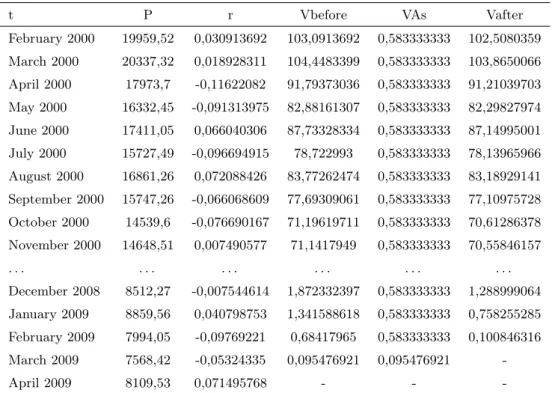
Table 1.2 shows how a basic VA contract operates. Suppose that the policyholder in-vests part of his/her savings in an immediate variable annuity contract depositing an amount of money equal, for the sake of simplicity, to $100 on the 1st February 2000. Among the available funds for the investment portfolio, the policyholder chooses to invest the entire premium in the Nikkei 225 index. Assume that the fixed annual withdrawal rate provided by the contract is equal to 7%, so the insured has the pos-sibility to withdraw $7 every year until the drawdown process will exhaust, sooner or later, the VA sub-account. Fulfilling the financial needs of the client, the insurance company makes monthly payments which amount to $(7/12) = $0.58333. In the table, the first column reports the life span of the contract split in monthly install-ments. In the second column historical prices of the index are recorded; in particular we have considered the closing prices recorded on the first day of each month and ad-justed to consider possible dividends payable. In the third column we have calculated the monthly index yield rate through the formula r= (Pt−Pt−1)/Pt−1, where Ptis
the index price at timet,Pt−1 is the index price at immediately before month. The
later columns recorded the value of the VA sub-account before (Vbefore) and after (Vafter) withdrawals and the amount of periodical withdrawals (VAs). The example underlines the effective dependence of the VA sub-account’s value on the investment portfolio’s performance, it being understood that the policyholder is still alive. For example, at the end of the first month considered, due to the positive return of the index, the value of the account increases from $100 to$(100(1 + 0.0309)) = $103.091. From this amount we have to deduct the monthly withdrawal, so that the account value becomes equal to $(103.091-0.5833) = $102.508. At the end of the third month, instead, the negative performance of the investment portfolio drives down the value of the account. We notice that on March 2009 the account value before withdrawals amounts to $0.09547. This sum of money is not sufficient to cover the periodic with-drawal equal to $0.58333. A standard VA policy, in this situation, runs out. The total withdrawals amount to $(109×0.5833 + 0.09547)= $63.092. It’s well-rendered
Table 1.2: How a basic variable annuity works
t P r Vbefore VAs Vafter February 2000 19959,52 0,030913692 103,0913692 0,583333333 102,5080359 March 2000 20337,32 0,018928311 104,4483399 0,583333333 103,8650066 April 2000 17973,7 -0,11622082 91,79373036 0,583333333 91,21039703 May 2000 16332,45 -0,091313975 82,88161307 0,583333333 82,29827974 June 2000 17411,05 0,066040306 87,73328334 0,583333333 87,14995001 July 2000 15727,49 -0,096694915 78,722993 0,583333333 78,13965966 August 2000 16861,26 0,072088426 83,77262474 0,583333333 83,18929141 September 2000 15747,26 -0,066068609 77,69309061 0,583333333 77,10975728 October 2000 14539,6 -0,076690167 71,19619711 0,583333333 70,61286378 November 2000 14648,51 0,007490577 71,1417949 0,583333333 70,55846157 . . . . December 2008 8512,27 -0,007544614 1,872332397 0,583333333 1,288999064 January 2009 8859,56 0,040798753 1,341588618 0,583333333 0,758255285 February 2009 7994,05 -0,09769221 0,68417965 0,583333333 0,100846316 March 2009 7568,42 -0,05324335 0,095476921 0,095476921 -April 2009 8109,53 0,071495768 - -
-the risks underlying -the contract. A prolonged negative performance of -the reference portfolio during the lifespan of the contract could preempt its end and consequently reduce the total withdrawals received by the policyholder. The same happens for example if the annuitant dies few years after the contract’s drafting, unlike his/her expectations. Just to face these risks that the VA market has begun to develop, insomuch as this class of annuities has achieved resounding success among investors. Many other features, in fact, contributed to make these products attractive.
The demand for this kind of policy is supported by two main factors: the pref-erential tax treatment and the possibility of underwriting several rider benefits that provide a protection of the policyholder’s savings account for the period before and after retirement.
The success of variable annuities is no doubt due to the presence of tax incentives, in-troduced by governments to support the development of individual pension solutions
and contain public expenditure. From a tax perspective, annuities have the following key features that until now were not available with other investment products:
- tax deferability of investment earnings until the commencement of withdrawals; interests, dividends and capital gains that accrue on assets held in variable annuity accounts, in fact, are not taxed until the policyholder receives its payouts. Thus, the sum invested in the contract can grow faster. This tax-advantaged treatment is not offered to variable annuities that are owned by a non-natural person, such as a corporation or certain trusts. In most USA traded VAs, when the policyholder takes his/her money out of a variable annuity, however, he/she will be taxed on the earnings at ordinary income tax rates rather than capital gains rates that might be lower. Moreover, if taken prior to age 5912, withdrawals may be subject to a 10% federal additional tax. In general, when a variable annuity is part of a retirement plan, the benefits of tax deferral will outweigh the costs only if the tax rate in the decumulation phase is lower than in the accumulation phase and the variable annuity is hold as a long-term investment to meet retirement and other long-range goals;
- favorable tax treatment of annuity income payments through the determination of an exclusion ratio to allow for a portion of each payment to be considered return of principal and a portion to be considered return of taxable investment earnings;
- tax-free transfer of funds between VA investment options. “Section 1035 exchanges” of the Internal Revenue Code in the USA allows a policyholder to make a direct transfer of accumulated funds in one annuity policy into another annuity policy without creating a taxable event; an individual can exchange one company’s prod-uct for another’s and the earnings from the original investment will remain tax deferred until the annuity owner withdraws money from the variable annuity con-tract;
- protection of VA assets from the insurance company’s creditors in the event of an insurer bankruptcy. The funds invested in a variable annuity contract are held in designed “sub accounts” that are kept separate from the insurance company’s
other assets. So the assets are not subject to claims by the insurance company’s creditors if it became insolvent.
In respect of traditional life insurance products, the main feature of variable annuities is the possibility of enjoying of a large variety of benefits represented by guarantees against investment and mortality/longevity risks. In particular, these products are designed to guarantee a minimum performance level of the underlying, thus protecting the policyholder against market downfalls, both in case of death and in case of life. Over the years, the guarantees offered on variable annuity products have evolved as the market has adapted to meet customer needs. While the vast majority of current variable annuities offers a death benefit rider as a default fea-ture, more sophisticated designs include a variety of living benefit riders. Available guarantees are usually referred to as GMxB, where “x” stands for the class of benefits involved. A first classification, as above mentioned, is between:
- Guaranteed Minimum Death Benefits (GMDB);
- Guaranteed Minimum Living Benefits (GMLB).
The Guaranteed Minimum Death Benefit (GMDB) is usually available during the accumulation period even if some insurers are willing to provide them also after retirement, up to some maximum age (say, 75 years). It addresses the concern that the policyholder may die before all payments are made. If it happens, the beneficiary receives a death benefit equal to the current asset value of the contract or, if higher, the guaranteed amount, which typically is the amount of premiums paid by the deceased policyholder accrued at the guaranteed rate.
In contrast, living benefits can be described as preservation or wealth-decumulation products as they enable the policyholder to preserve wealth during the drawdown period. There are three common types of living benefit riders:
- Guaranteed Minimum Accumulation Benefits (GMAB);
- Guaranteed Minimum Income Benefits (GMIB);
The Guaranteed Minimum Accumulation Benefit (GMAB) is designed as a wealth-accumulation product, available prior to retirement. It guarantees that the final con-tract value at the end of the accumulation phase will not fall below a specific level regardless of the actual investment performance. This type of guarantee is particu-larly enticing to younger investors.
The other living benefits focus on the decumulation or payout phase of a variable annuity.
The Guaranteed Minimum Income Benefit (GMIB) rider is designed to provide the investor with a base amount of lifetime income at retirement, which is at least as valuable as the account value of the investments at the point of conversion. Triggering this guarantee is similar to purchasing an annuity in the traditional sense.
The Guaranteed Minimum Withdrawal Benefit (GMWB) riders guarantee that a certain percentage (usually 5% to 7%) of the invested premium can be withdrawn annually until the entire amount is completely recovered, regardless of market per-formance. So periodical withdrawals are allowed even if the account value reduces to zero because of bad investment performances. The contract may include clauses that serve to discourage excessive withdrawal. For example, when the policyholder withdraws at a higher rate than that contractually specified, the guarantee level could be reset to the minimum of the prevailing guarantee level and the account value. Also a percentage penalty charge could be applied on the excessive portion of the withdrawal amount. In this work we will refer to this last rider, and to be more precise, to its ultimate version, represented by the Guaranteed Lifetime Withdrawal Benefit.
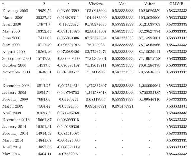
To facilitate the understanding of the GMWB policy, in Table 1.3 we consider its workings through a numerical example. Consider the same policy described in Ta-ble 1.2 adding a GMWB rider. With this supplementary option, the policyholder preserves the possibility to withdraw the same amount until the contract maturity, also in case of a market drawdown. So, in the example, at the end of the 109th pe-riod (March 2009), the guarantee becomes effective and ensures a stream of monthly payments equal to $0.5833 until the initial premium has been totally recouped. This
happens(100/0.5833) = 171.44months (171.44/12 = 14.28years) after the initiation of the contract. Therefore, adding a GMWB rider to a standard variable annuity contract, the policyholder is really provided against the negative performance of the investment portfolio.
Note that a key advantage of the Guaranteed Withdrawal Benefit (GWB) feature over other VA based options available in the market is that in GWB the underlying investment can continue to have market exposure even when the withdrawals start and thus has a greater growth opportunity. In contrast, with other widely marketed VA based options such as the GMAB or the GMIB/GAO, the underlying investment is effectively annuitized or invested in fixed income instruments upon maturity.
As a result of rising life expectancies as well as increases in lifestyle and health-care costs, retirement lifespans have become both longer and more expensive. At the same time, with the social security system under considerable stress, the idea that individuals and households need to plan for their own retirement is gaining traction. To satisfy these new needs insurance companies have started offering a life-time benefit feature with GMWB, enabling the investor to simultaneously manage both financial as well as longevity related risks. GMWB with lifetime withdrawals is commonly known as “Guaranteed Lifetime Withdrawal Benefits” (GLWB) or “Guar-anteed Withdrawal Benefits (GWB) for life”. This rider guarantees policyholders the possibility of withdrawing an annual amount (typically 4% to 7%) of their guaranteed protection amount (GLWB Base) for their entire lifetime, no matter how the invest-ments in the sub-accounts perform. It’s the only product that combines longevity protection with withdrawal flexibility, hence it is seen as a “second-generation” guar-antee. The guarantee can concern one or two lives (typically spouses). Each annual withdrawal does not exceed some maximum value, but it is evident that the to-tal amount of withdrawals is not limited, depending on the policyholder’s lifetime. Annual withdrawals of about 5% of the (single initial) premium are commonly guar-anteed for insured aged 60+. In case of death any remaining fund value is paid to the insured’s dependants. In deferred versions of the contract, the product is fund linked during the deferment and the account value at the end of this period, or a
Table 1.3: How works a variable annuity with a GMWB rider
t P r Vbefore VAs Vafter GMWB February 2000 19959,52 0,030913692 103,0913692 0,583333333 102,5080359 0,583333333 March 2000 20337,32 0,018928311 104,4483399 0,583333333 103,8650066 0,583333333 April 2000 17973,7 -0,11622082 91,79373036 0,583333333 91,21039703 0,583333333 May 2000 16332,45 -0,091313975 82,88161307 0,583333333 82,29827974 0,583333333 June 2000 17411,05 0,066040306 87,73328334 0,583333333 87,14995001 0,583333333 July 2000 15727,49 -0,096694915 78,722993 0,583333333 78,13965966 0,583333333 August 2000 16861,26 0,072088426 83,77262474 0,583333333 83,18929141 0,583333333 September 2000 15747,26 -0,066068609 77,69309061 0,583333333 77,10975728 0,583333333 October 2000 14539,6 -0,076690167 71,19619711 0,583333333 70,61286378 0,583333333 November 2000 14648,51 0,007490577 71,1417949 0,583333333 70,55846157 0,583333333 . . . . December 2008 8512,27 -0,007544614 1,872332397 0,583333333 1,288999064 0,583333333 January 2009 8859,56 0,040798753 1,341588618 0,583333333 0,758255285 0,583333333 February 2009 7994,05 -0,09769221 0,68417965 0,583333333 0,100846316 0,583333333 March 2009 7568,42 -0,05324335 0,095476921 0,095476921 - 0,583333333 April 2009 8109,53 0,071495768 - - - 0,583333333 December 2013 15661,87 0,093099915 - - - 0,583333333 January 2014 16291,31 0,040189326 - - - 0,583333333 February 2014 14914,53 -0,084510085 - - - 0,583333333 March 2014 14841,07 -0,004925398 - - - 0,583333333 April 2014 14827,83 -0,000892119 - - - 0,583333333 May 2014 14304,11 -0,03532007 - - - 0,583333333
guaranteed amount if greater, is treated like a single premium paid for an immediate GLWB.
As noted earlier, the Benefit Base is the figure the policyholder’s future guaran-teed income payments will be based on. Typically, in all rider benefits described, it initially equals the contributions made to the annuity. However, during the lifetime of the contract, it could be a different sum because of additional features offered with GMxBs.
For example, if a roll-up is included within the policy, the annual guaranteed amount is increased by a fixed percentage every year during a certain time period but only if the policyholder has not started withdrawing money. Therefore, roll-ups are commonly used as an incentive to the policyholder not to withdraw money from the account in the first years. Usually the minimum rate of growth is 5% - 7%.
The amount guaranteed for withdrawal may also depend on the account value and increase during the policy lifespan if the fund’s assets perform well, allowing the policyholder to withdraw a higher amount than that initially guaranteed. This increase may either be permanent or be effective just for the single withdrawal. The step-up feature, in particular, can increase the benefit base amount if the VA account value after withdrawals is higher than the benefit base on specified dates. Typically, step-up dates are annually or every three or five years on the policy anniversary date. Therefore, step-ups only occur if the policyholder’s funds yield high performance and the account value has not been decreased heavily due to previous withdrawals. Com-mon step-up features are, e.g., annual ratchet guarantees. Regarding this feature, four different product designs can be observed in the market (Kling et al. (2011)):
- No Ratchet. In this case no ratchets or surplus exist at all; the guaranteed annual withdrawal is constant and does not depend on market movements;
- Lookback Ratchet. This alternative considers a withdrawal benefit base at outset given by the single premium paid. During the contract term, on each policy an-niversary date, the benefit base is compared with the account value at that time. The higher value among them is taken as the new benefit base. So, if the account value at a certain date exceeds the previous benefit base, the guaranteed withdrawal
is increased accordingly to the preset percentage multiplied by the new withdrawal benefit base. This effectively means that the fund performance needs to compen-sate for policy charges and annual withdrawals in order to increase the guaranteed withdrawals. With this product design, increases in the guaranteed withdrawal amount are permanent, i.e. over time, the guaranteed withdrawal amount may only increase, never decrease;
- Remaining Withdrawal Benefit Base Ratchet. As in the previous case, the with-drawal benefit base at outset is given by the single premium paid. The withwith-drawal benefit base is however reduced by every guaranteed withdrawal. As before, on each policy anniversary, if the account value exceeds the benefit base, the new benefit base is increased to the account value. The guaranteed annual withdrawal is however increased by the preset percentage multiplied by the difference between the account value and the previous benefit base. This effectively means that, in order to cause an increase of guaranteed annual withdrawals, the fund performance needs to compensate for policy charges only but not for annual withdrawals. This ratchet mechanism, other things being equal, is therefore somewhat “richer” than the Lookback Ratchet. Therefore, typically the initially guaranteed withdrawal amount should be lower than with a product offering a Lookback Ratchet. As with the Lookback Ratchet design, increases in the guaranteed amount are perma-nent;
- Performance Bonus. For this alternative the withdrawal benefit base is never in-creased. On each policy anniversary date, in fact, if the current account value is greater than the current withdrawal benefit base, 50% of the difference is added to this year’s guaranteed amount as “performance bonus”. In contrast to the pvious two designs, therefore, in this case the guaranteed withdrawal amounts re-main unchanged. For the calculation of the withdrawal benefit base, only annual withdrawals are subtracted from the benefit base and not the performance bonus payments.
it gives the opportunity to renew the option when it reaches maturity, so it allows to postpone the maturity date; in a GMDB, instead, it allows the guaranteed with-drawal amount to equal the account value at some prior specified date, note as reset dates. In this case, unlike the ratchet guarantee, the minimum guaranteed amount may decrease if the account value falls off between two reset dates.
One of the most common options available in policies with a considerable savings component as variable annuities is the possibility to exit (surrender) the contract before maturity and to receive a lump sum (surrender value) reflecting the insured’s past contributions to the policy, minus any costs incurred by the company and pos-sibly some charges. The idea is to boost sales by ensuring that the policyholder does not perceive insurance securities as an illiquid investment. At the same time, how-ever, surrenders are not welcome by insurers, as they imply a reduction in the assets under management and may generate imbalances in the exposure to the mortality risk of remaining insureds (selective surrenders). For these reasons, there are often surrender penalties that apply if funds are withdrawn before a pre-specified time period, often seven years. These penalties, known as Contingent Deferred Surrender Charges (CDSC), can be several percent of the annuity’s value.
This is a simplified description of the basic design of the guarantees embedded in VAs; a complete description of all possible variants would be beyond the scope of this thesis, focused on the actuarial and financial valuation of this kind of contracts. Thus, some products offered in the market may have features different from those investigated above or may be a combination of two or more guarantees. The reader interested in a detailed overview of variable annuities could refer to Ledlie et al. (2008).
Insurance companies charge a fee for the offered benefits. Guarantees and asset management fees, administrative cost and other expenses are charged typically de-ducting a certain percentage of the underlying fund’s value from the policyholder’s funds account on an annual basis. Very rarely they are charged immediately as a single initial deduction. This improves the transparency of the contract, as any deduction to the policy account value must be reported to the policyholder. Some
guarantees can be added or removed, at policyholder’s discretion, when the contract is already in-force. Accordingly, the corresponding fees start or stop being charged. Unlike most “good” investments, VAs’ fees are quite high. For this reason, they used to receive heaps of bad press. Also investors don’t look kindly upon this aspect, because of the combination of investment management and insurance expenses sub-stantially reduces their returns. Analyzing many VA contracts traded in USA it’s possible to classify insurance charge into many categories:
- mortality and expense risk charge (M&E). The M&E charge compensates the in-surance company for inin-surance risks and other costs it assumes under the annuity contract. The fees for any optional death and/or living benefit the policyholder may select are described below and are not included in the M&E charge. M&E charges are assessed daily and typically range from 1.15% to 1.85% annually;
- administrative and distribution fees. These fees cover the costs associated with servicing and distributing the annuity. They include the costs of transferring funds between sub accounts, tracking purchase payments, issuing confirmations and statements as well as ongoing customer service. These fees are assessed daily and typically range from 0% to 0.35% annually;
- contract maintenance fee. It is an annual flat fee charged for record-keeping and administrative purposes. The fee typically ranges from $30 to $50 and is deducted on the contract anniversary. This fee is typically waived for contract values over $50.000;
- underlying sub account fees and expenses. Fees and expenses are also charged on the sub accounts. These include management fees that are paid to the invest-ment adviser responsible for making investinvest-ment decisions affecting investor’s sub accounts. This is similar to the investment manager’s fee in a mutual fund. Ex-penses include the costs of buying and selling securities as well as administering trades. These asset-based expenses will vary by sub account and typically range from 0.70% to 2.50% annually;
- contingent deferred sales charge (or surrender charge). Most variable annuities do not have an initial sales charge. This means that 100% of funds are used for immediate investment in the available sub accounts. However, insurance companies usually assess surrender charges to annuity owners who liquidate their contract (or make a partial withdrawal in excess of a specified amount) during the surrender period. The surrender charge is generally a percentage of the amount withdrawn and declines gradually during the surrender period. A typical surrender schedule has an initial surrender charge ranging from 7% to 9% and decreases each year that the contract is in force until the surrender charge reaches zero. Generally, the longer is the surrender schedule, the lower are the contract fees. Most contracts will begin a new surrender period for each subsequent purchase payment, specific to that subsequent purchase payment.
- fees and charges for other features. Special features offered by some variable annu-ities, such as a stepped-up death benefit, a guaranteed minimum income benefit, or long-term care insurance, often carry additional fees and charges.
First introduced in the US in the early 1970s, variable annuities quickly expe-rienced remarkable growth. In recent years, they have become very popular life insurance products, able to address the long-term savings and retirement needs of a rapidly aging population. As individuals also become more heterogeneous in terms of their demand characteristics, there is growing recognition in the industry and by governments that existing retirement models have to be improved to better meet consumer needs. In particular, consumers require access to market returns in order to keep pace with the rising cost of living, but they also need to protect their assets and lifestyle from negative economic trends. Variable annuities represent a valuable compromise, and their commercial features make them attractive, providing a good opportunity for market development.
However, caution is necessary because variable annuities can have a high negative impact on the VA provider’s balance sheet. If the GWxB is significantly underpriced or raises the possibility of a debilitating loss for the underwriting company, then the related credit-worthiness issue should make potential clients skeptical of the product.
Therefore, for the long term sustainability of GWxBs it is important that the compa-nies offering them remain profitable and viable. A proper risk management process is consequently needed. It usually requires several phases, from the risk identification, to its assessment, to the choice of (a mix of) risk management techniques. If fairly priced, the GWB for life option is an attractive retirement solution for investors as it allows them to manage the risks related to their own longevities, which cannot be mitigated at an individual level. Further, the ability to stay invested in the market while in retirement would allow investors to better cope with the inflation related risk, which becomes significant as the retirement lifespans get longer.
1.4
Risks underlying Variable Annuities
From the above description it is clear that several risks affect the performance of a VA contract. In addition to risks which are typically implied by life-insurance products, such as mis-selling risks, the risks arising from mis-specified policy conditions or other sales material, regulatory and accounting risks, etc., there are risks which are specific to VAs (Kalberer & Ravindran (2009)). These can be classified into three categories:
• shortfall risks. This category includes two kinds of risks. The first one con-cerns the possibility that the performance of the underlying asset is insufficient to cover the guarantees given a certain expected realisation of biometric2 (or more general, insurance) risk, e.g. a certain pattern of expected deaths or sur-render. The second kind of risk is linked to the chance that biometric factors insured (e.g. death) develop adversely such that even an asset performance able to cover the guarantees in the expected case becomes insufficient. This happens, for example, when longevity exceeds expectations. These two kinds of risks are evidently connected. So even if the biometric risk can be minimised
2
Underwriting risks covering everything related to human life conditions, e.g. death, disability, longevity, but also birth, marital status, age, and number of children (e.g. in collective pension schemes).
through diversification, the risk from the asset part has to be hedged through instruments that are dependent on both asset and biometric developments in a combined way, and such investments typically do not exist (and are definitely not liquid traded);
• pricing risk. It is the risk that the price of the guarantees may be inadequate. There are two methods to evaluate the premium charged by the insurance company:
- a theoretical approach, through which the price should cover the theo-retical value of the guarantee, consistent with the insights of financial economics. Such a premium, however, couldn’t consider frictional costs which arise in practice, like transaction costs, bid-offer spreads or simply the fact that the requirements of a theoretical model are rarely really ful-filled, e.g. continuous re-hedging, complete markets, no cost of capital, etc. So the premium charged could be insufficient to hedge the exposure properly. The model underlying the pricing might also be inadequate or insufficiently calibrated; this is called the “model risk”;
- an hedging approach, through which the price should be just sufficient to cover the costs of hedging. But also in this case many risks emerge. It could happen that available hedging instruments used for pricing do not really replicate the exposure (replication risk). Moreover, not always prices of the hedging instruments are readily available and theoretical models have to be used to determine their prices, so the same problems presented in the previous case emerge. Also the policyholder behaviour has a hold on the premium charged by the insurance company. In fact, when determining the right price for the guarantee, a certain amount of policyholder lapsation3 is expected. If a policyholder lapses, then he/she loses his/her guarantees in most cases, such that a certain amount of
3
Lapsation of a life insurance policy is discontinuation of premium payment by the policyholder during the life span of the policy.
lapsation results in a lower overall cost for the guarantees. This implies lower (and thus more competitive) prices. Policyholders, however, are assumed to act financially rationally. In particular, when the value of the underlying funds is low and consequently the value of the guarantee is high, being guarantee charges fixed, policyholders will feel inclined to stay and not to lapse their contract (“in-the-money persistency”). Conversely, if the value of the underlying funds is high (in relation to the guarantees), then the value of the guarantees will be low, even vanishing in extreme cases. Policyholders will thus feel inclined to lapse and avoid the now unnecessary guarantee charges (“out-of-the money lapsation”). Thus, the lapsation will be asset dependent. This should be reflected in the pricing assuming a certain policyholder behaviour. But this behaviour has not been explored in depth and can change over time. The resulting risk is called “policyholder behaviour risk”;
• hedging risk. It is the possibility that risk management strategies may fail. A dynamic-hedging programme requires the creation of a hedge portfolio which tightly follows the value of the guarantees. And the value of the guarantees is dependent on a whole range of parameters, for example the features of the guarantee, the value of the underlying assets, the volatility of the underlying funds, the interest rates in the policy currency, the proportion of surviving policyholders, and potentially much more. In turn, some of these parameters are dependent on more basic parameters, e.g. the value of the underlying funds is dependent on the value of the components of the funds in their denomina-tion currency, the exchange rate between denominadenomina-tion currency and policy currency, the size and timing of dividends of the underlying assets and so on. The general risk of a hedging strategy is that the development of the hedging portfolio deviates from the development of the value of the guarantees. The risks involved are, among others:
the underlying funds increases in an unforeseen way over time, resulting in losses when trying to roll over a potential hedge of the product;
– interest rate risk. It is the risk that the level of interest rates changes. It can in most cases be hedged away quite efficiently through a wide range of instruments available in the market, such as long-term swaps;
– gamma risk. Gamma measures the rate of change of Delta as the under-lying moves. Delta tells us how much an option price will change given a one-point move of the underlying. But since Delta is not fixed and will increase or decrease at different rates, it needs its own measure, which is Gamma;
– foreign exchange risk. It is the risk that the guarantee is denominated in a policy currency which is different from that of the underlying funds, such that not only the asset performance of the underlying funds but also the fluctuations between the two currencies must be hedged;
– basis risk. It is the risk which emerges when there exist no hedging instru-ments on the underlying assets and so the solution is to map the funds to a portfolio of assets which can be hedged, typically consisting of stock market indexes, also called the “benchmark portfolio”. A special case of this risk is the “dividend risk”, which arises when the amount of dividend payments on the benchmark assets fluctuates causing hedging deviations. Another example of basis risk is the “correlation risk”. The volatility of the benchmark index, in fact, depends on the correlation between the asset indexes forming the benchmark portfolio; thus, changes in this correlation can result in hedging losses;
– funds choice risk. Usually the policyholder has the contractual right to choose the underlying funds from a prescribed list of available funds and exchange funds at market value, paying a relatively small handing fee. But some of the funds in the list could be not hedgable, and their basis risk could be so high that it exceeds the benefits of hedging;
– policyholder behaviour risk. It emerges when the asset dependent policy-holder behaviour differs from that supposed when determining the hedging portfolio, e.g. assuming a certain percentage of lapses;
– liquidity risk, because of market constraints, hedging instruments which were initially liquid could become illiquid over time or even cease to exist;
– counterparty credit risk. The hedging instruments, e.g. swaps, involve counterparties which may fail to serve their obligations;
– key-person risk. It is the risk that the necessary skills and know-how required to set up a dynamic hedging programme couldn’t be retained during the whole life of the hedging operations, a time which can easily exceed 30 years;
– operational risk. It is the risk remaining after determining financing and systematic risk, and includes risks resulting from breakdowns in inter-nal procedures, people and systems. The hedging programme typically consists of a complex series of processes, some of them IT (information technology)-related. These processes must be performed regularly in a timely manner and without mistakes. The operational risk involved is considerable and exceeds the typical level in an insurance company;
– transaction cost risk. Hedging operations require regular transactions, which are typically associated with transaction costs, e.g. in the form of bid-offer spread;
– cost of capital risk. VA products are under scrutiny from regulators, who typically require a substantial amount of risk capital. Regulations may change over time because of developments out of the control of an indi-vidual insurance company, such as political developments or insolvencies of competitors. So, risk capital requirements may increase, causing a need for liquidity and higher costs of capital for VA products;
– cost of risk-management risk;
the risk exposure of VAs or new VA features and regard the company’s financial situation as more opaque when exposed to VAs. These exposures could not be communicated adequately to investors. The result is an increase of the premium.
Note that this is only a partial overview of all possible risks involved. It is important to notice that the risks associated with a VA are typically not eliminated but only transformed. One risk is replaced with another, hopefully more easily manageable risk.
1.5
Variable annuities during the recent market Crisis
The recent severe financial crisis in 2007-2008 highlighted all the risks of variable annuities. Not only life insurers have experienced realized and unrealized losses in their general accounts from credit exposures, but their VA businesses have created exposures to equity markets that have threatened the survival of some and put pres-sure on the business model and balance sheet of others.
Let’s revisit briefly the fundamental changes in VA sales in the US market over the last 20 years (Chopra et al. (2009))
Before the 1990s, dividend and capital gains tax rates were higher and largely in line with marginal tax rates, so variable annuities were considered appealing because they offered policyholders the possibility to accumulate higher levels of tax-deferred savings within a life insurance policy. The 1990s saw the growth of available invest-ment choices and enhanceinvest-ments of death benefits, which resulted in asset growth of 21 percent per year, with assets reaching almost $1 trillion by the end of 2000. By 2003, affluent baby-boomers began approaching middle age with swelling 401(k) balances4and limited ability to protect themselves against longevity and market risk. Changes in tax rates also weakened the traditional appeal of variable annuities as a
4
A 401(k) plan is a qualified (i.e., meets the standards set forth in the Internal Revenue Code (IRC) for tax-favored status) profit-sharing, stock bonus, pre-ERISA money purchase pension, or a rural cooperative plan under which an employee can elect to have the employer contribute a portion of the employee’s cash wages to the plan on a pre-tax basis. These deferred wages (elective deferrals)
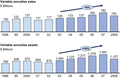
Figure 1.1: Variable annuities 1998-2008
4
It is worth recalling also that the variable annuity has undergone fundamental changes over the last
20 years. From a straightforward product at its inception, it has evolved into a complicated financial instrument with significant risk exposures for the manufacturer. Four trends drove this transformation.
1. “ARMS RACE” ON LIVING BENEFITS
Before 2003, and in particular before the 1990s, when dividend and capital gains tax rates were higher and largely in line with marginal tax rates, variable annuities offered policy holders a chance to accumulate higher levels of tax-deferred savings within a life insurance wrapper.
The 1990s saw the broadening of available investment choices and enhancements to death
benefits, which resulted in asset growth of 21 percent per year, with assets reaching almost
$1 trillion by the end of 2000.
By 2003, affluent baby-boomers began approaching middle age with swelling 401(k) balances and
limited ability to protect themselves against longevity and market risk. Changes in tax rates also weakened the traditional appeal of variable annuities as a tax deferral vehicle, and growth started
to flatten. These forces pushed the industry aggressively to develop and market new guarantees
promising continued tax deferral (similar to 401(k) and other IRA vehicles) while also offering market and longevity protection to policyholders.
06 07 2008
+9%
1998 99 2000 01 02 03 04 05
Variable annuities assets
$ Billions
Variable annuities sales
$ Billions 1998 +10% 2008 04 05 06 07 99 2000 01 02 03
Source: LIMRA survey (1998-2007); Morningstar (2008); analyst reports
Variable annuities 1998-2008 Exhibit 1 769 100 122 137 111 117 129 133 137 160 182 152 949 972 904 815 1,004 1,123 1,217 1,379 1,491 1,127
tax deferral vehicle, and growth started to flatten. These forces led to a development of the insurance industry. In the early 2000s guaranteed living benefits were intro-duced. Living benefits provided a threshold of payments that policyholders could receive either during the accumulation or withdrawal phase (depending on the type of living benefit), regardless of their lifespan. The introduction of these guarantees set off a period of rapid development in which the market saw waves of new products with increasingly sophisticated guarantees. This innovation generated significant customer interest because it allowed clients to protect their investment from equity market declines. The introduction of the Guaranteed Withdrawal Benefit for Life in 2005 created a new standard for the industry, combining the longevity protection with the liquidity of the regular withdrawal benefit. Importantly, the introduction of these living benefits took place in the context of rising stock markets: a wave of bene-fits were launched beginning in 2002 and continuing to 2007, a period when the S&P 500 index grew at 9 percent per year. Hence, the period of 2003-07 was an excep-tionally strong one for the life insurance industry. Figure 1.1 shows variable annuity
are not subject to federal income tax withholding at the time of deferral and they are not reflected as taxable income on the employee’s Individual Income Tax Return.
sales grew by around 9 percent annually over 2003-2007 (approximately $50 billion total), increasing assets to about $1.5 trillion by 2007. In some sense, VAs emerged as the natural product for affluent investors in their 50s and 60s as they transitioned from the accumulation to the decumulation stage of their investment lifecycle. With the introduction of living benefits and market performance guarantees, policyholders used variable annuities as a vehicle to invest in mutual funds. Investment choices in VAs began more and more focused on equity. Ferocious competition among VA play-ers, intensified by the growing importance of independent sales channels, led many insurers to issue ever more generous guarantees at ever lower prices. When the crisis hit, the assumptions underlying their calculations - from equity market volatility to customer conduct - proved to be unrealistic. The sharp rise in the volatility of the stock market, in particular, led to a dramatic increase in the costs of hedging VA business. Because of significant declines in equity values, most guarantees embedded in VAs have become in-the-money, entailing losses for the issuer. This resulted in higher rider fees in new VA products. Potential policyholders, however, were not attracted by these higher prices, so sales reduced. Moreover, as fees are based on the actual account values, the considerable fall in equity prices has significantly re-duced insurer’s income streams. As a result, many companies’ credit ratings were downgraded by the rating agencies.
However, the most important consequence of the market crisis is related to risk management and hedging programs. Considering that the guarantees from existing products have become more valuable and more likely to end up the-money, in-surance companies providing them with have been forced to raise their risk-based capital requirement. As a consequence, hedging programs, which are used to counter this increase in liabilities or reinsurance arrangements for risk transfer, have gained importance. Generally, funds cannot be hedged directly, for this reason they are mapped to hedgeable indices or risk factors. This mapping is often based on simple linear relationships determined by historical data. However, during extreme market fluctuations this simple approach has often caused basis mismatches (deviations be-tween funds and corresponding indices), which have contributed directly to hedge
ineffectiveness. Now there is an increasing tendency to include investment funds that employ different risk mitigation strategies in VA policies. Examples of these types of funds are volatility target funds and funds with a built-in downside protection. These allow VA guarantee costs to be shifted to the fund level. To avoid further guarantee costs and to benefit fully from these risk management strategies, it is es-sential to model these funds properly by using advanced mapping techniques and accounting for the current fund allocation.
Many insurers are still raising prices, decreasing benefits and features, discontin-uing products and, in some cases, even exiting the business. Despite the somewhat steady growth of the US economy in early 2012, the global economic outlook looks less certain. During the first quarter of 2012, Hartford Life announced that it will no longer sell variable annuities. This follows the exit of Sun Life, Genworth and ING in 2011, and the scale-back by MetLife through 2011 and 2012. Consequently, distrib-utors are now very sensitive to the possibility that a company may not offer variable annuities in the future. Product trends in 2012 continue to focus on restructuring living benefits on VA. Some companies have decreased the withdrawal percentages and bonuses, increased the charges or made the investment options more restrictive. Others have introduced new, less-competitive benefits and pulled the richer ones from the market. Insurance companies continue to look for new ways to de-risk, such as managing volatility within the funds or even buying back certain benefits. Neverthe