University of Wisconsin Milwaukee
UWM Digital Commons
Theses and DissertationsMay 2018
Optimization for Integration of Plug-in Hybrid
Electric Vehicles into Distribution Grid
Shuaiyu Bu
University of Wisconsin-Milwaukee
Follow this and additional works at:https://dc.uwm.edu/etd
Part of theElectrical and Electronics Commons
This Thesis is brought to you for free and open access by UWM Digital Commons. It has been accepted for inclusion in Theses and Dissertations by an authorized administrator of UWM Digital Commons. For more information, please [email protected].
Recommended Citation
Bu, Shuaiyu, "Optimization for Integration of Plug-in Hybrid Electric Vehicles into Distribution Grid" (2018).Theses and Dissertations. 1763.
OPTIMIZATION FOR INTEGRATION OF PLUG-IN HYBRID ELECTRIC VEHICLES INTO DISTRIBUTION GRID
by Shuaiyu Bu
A Thesis Submitted in Partial Fulfillment of the Requirements for the Degree of
Master of Science in Engineering
at
The University of Wisconsin-Milwaukee May 2018
ii ABSTRACT
OPTIMIZATION FOR INTEGRATION OF PLUG-IN HYBRID ELECTRIC VEHICLES INTO DISTRIBUTION GRID
by Shuaiyu Bu
The University of Wisconsin-Milwaukee, 2018 Under the Supervision of Dr. Lingfeng Wang
Plug-in hybrid electric vehicles (PHEVs) feature combined electric and gasoline powertrains with internal combustion engine and electric motors powered by battery packs. The battery packs of PHEVs are mostly charged during off-peaks hours at lower prices and meanwhile absorb the excess power from the grid. Similarly, the power stored in the batteries can also flow back to the electric grid in response to ease the peak load demands.
With the increasing penetration and integration of PHEVs, the reliability of PHEVs is essential to overall power system reliability since the charging mechanisms of PHEVs can influence the reliability of power system. Furthermore, due to the direct integration of PHEVs into the residential distribution network, the PHEVs can work as backup batteries for power systems in case of power outage. Therefore, the reliability analysis of power systems and the ancillary services provided by PHEVs are also proposed in this thesis study.
For the driving pattern of each PHEV, there are three basic elements modeled, which are the departure time, the arrival time and the daily mileage, all represented by probability
iii
density functions. Based on these basic concepts, the methodology for modeling the load demand of PHEVs is introduced.
In the proposed system, both the Differential Evolution and the Particle Swarm Optimization are proposed to optimize the control strategies for power systems with integration of PHEVs. Aside from using the minimum cost as a figure of merit when designing and determining the best PHEV charging mechanism, the reliability improvement brought to the power systems by PHEVs and the extra earnings obtained by performing frequency regulation services are also quantified and taken into account. Although the reliability of power systems with PHEV penetrations has been well-studied, the adoption of the Differential Evolution algorithm for minimizing the cost of overall system is not exercised, not to mention a thorough comparative study with other common optimization algorithms. To sum up, the Differential Evolution can not only achieve multiple goals by improving the power quality, reducing the peak load, providing regulation services and minimizing the total virtual cost in this system, it can also offer better results compared with the Particle Swarm Optimization in terms of minimizing the cost.
iv
© Copyright by Shuaiyu Bu, 2018 All Rights Reserved
v
TABLE OF CONTENTS
Introduction ... 1
1.1 Research Background ... 1
1.1.1 Introduction of Plug-in Hybrid Electric Vehicles ... 1
1.1.2 Power System and Power System Reliability ... 2
1.1.3 Reliability Cost and Reliability Worth ... 3
1.1.4 Types of Electric Vehicles ... 4
1.1.5 The concept of Vehicle-to-Grid ... 6
1.1.6 Demand Response ... 7
1.1.7 Power Markets and Ancillary Services ... 8
1.2 Reliability Evaluation Method ... 10
1.2.1 Analytical Method ... 11
1.2.2 Simulation Method ... 11
System Model ... 13
2.1 Introduction ... 13
2.2 PHEV Load Demand ... 13
2.2.1 Predicted Driving Pattern ... 13
2.2.2 Stochastic Fuzzy Model ... 14
2.2.3 Initial SOC ... 16
2.2.4 PHEV Load Profile ... 17
2.3 Distribution System Model ... 17
2.3.1 Introduction ... 17
2.3.2 Residential Distribution System ... 19
2.4 Pricing Model ... 20
2.4.1 Pricing Scenarios ... 20
2.4.2 The Model of Battery Degradation Cost ... 22
2.5 Mathematics Models and Objective Function ... 23
2.5.1 Mathematics Models ... 23
2.5.2 Objective Function ... 24
Power System Reliability Analysis Methodology ... 26
3.1 Overview of Approach ... 26
3.2 Optimize Algorithms ... 26
3.2.1 Genetic Algorithm ... 27
3.2.2 Differential Evolution ... 31
3.2.3 Particle Swarm Optimization ... 33
3.3 Conclusions and Future Work ... 36
Simulation Results and Case Study ... 37
4.1 Simulation Results ... 37
4.1.1 Cost Results ... 37
4.1.2 Load Demand of Simulations ... 38
4.1.3 Comparison of Load Voltage ... 41
4.1.4 Peak Load ... 44
4.2 Case Study ... 44
4.2.1 The total cost In Different Pricing Scenarios ... 45
vi
Conclusion ... 47 References ... 49
vii
LIST OF FIGURES
Figure 1-1 Hierarchical Levels of Power System. ... 3
Figure 1-2 Utility Cost, Consumer Cost and Total Cost. ... 4
Figure 1-3 Schematic of control connections between PHEVs and power grid. ... 7
Figure 2-1 Load profile Model. ... 17
Figure 2-2 Topology of IEEE 34-node test feeder... 19
Figure 2-3 Real-time charging pricing tariff. ... 20
Figure 2-4 Time-of-use charging pricing tariff. ... 22
Figure 3-1 The flow diagram of Genetic Algorithm. ... 31
Figure 4-1 Load demand curves for different charging algorithms at 10% PHEV penetration level. ... 39
Figure 4-2 Load demand curves for different charging algorithms at 20% PHEV penetration level. ... 40
Figure 4-3 Load demand curves for different charging algorithms at 50% PHEV penetration level. ... 40
Figure 4-4 Load demand curves for different charging algorithms at 100% PHEV penetration level. ... 41
Figure 4-5 Voltage curves of IEEE 34-node test feeder for different charging algorithms at 10% penetration level. ... 42
Figure 4-6 Voltage curves of IEEE 34-node test feeder for different charging algorithms at 20% penetration level... 42
Figure 4-7 Voltage curves of IEEE 34-node test feeder for different charging algorithms at 50% penetration level. ... 43
viii
Figure 4-8 Voltage curves of IEEE 34-node test feeder for different charging algorithms at 100% penetration level. ... 43 Figure 4-9 Load demand curves for different charging algorithms at 50% PHEV penetration level. ... 45
ix
LIST OF TABLES
Table 1-1 Percentage of PHEVs with different AER. ... 6 Table 2-1 Constants in distribution functions of departure time, arrival time and daily mileage. ... 14 Table 4-1 Charging Cost, Regulation Earnings and Total Cost results with Differential Evolution. ... 37 Table 4-2 Charging Cost, Regulation Earnings and Total Cost results with Particle Swarm Optimization. ... 38 Table 4-3 Peak load of DE and PSO in different penetration levels. ... 44 Table 4-4 The cost result after adding V2G into simulation. ... 45 Table 4-5 The comparison of Time-of-use and Real-time pricing scenarios in different penetration levels. ... 46
x
ACKNOWLEDGEMENTS
First of all, I would like to express my deepest appreciation to my thesis advisor Dr. Lingfeng Wang for guiding me to research on such an important topic of these days. This thesis would not have been completed without his help, patience and support. He gives me valuable insights into various aspects in power and reliability fields, and his tireless efforts in research and academics also inspires me.
Furthermore, I wish to thank professors, Professor Jun Zhang, Professor Wei Wei, who attended my dissertation committee with their consistent support, suggestions and directions.
I would also like to express my sincere gratitude to my friends for their suggestions in my research. I was touched deeply by their accompany and support.
Finally, I would like to appreciate the financial support and love from my family, who always stand by me and encourage me.
1
Introduction
1.1 Research Background
1.1.1 Introduction of Plug-in Hybrid Electric Vehicles
As the fossil fuel energy becoming increasingly scarce, technologies that have potential to reduce energy use are evaluated. Since the transportation sector accounts for about two-thirds of the gasoline consumption in United States, new transportation technologies are booming, especially the application of Plug-in Hybrid Electric Vehicles (PHEVs).
Plug-in hybrid electric vehicles (PHEVs) feature combined electric and gasoline powertrains with internal combustion engine and electric motors powered by battery packs. The battery pack of PHEVs can be charged by plugging vehicles into the power grid and using excess engine power. Furthermore, due to the battery pack of PHEVs as well as the directly connections between PHEVs and power grid, PHEVs can work as backup batteries to power system when power outage happened.
Additionally, PHEVs have great potential to reduce oil consumption and greenhouse gases emission. With using electricity grids as a substitute for burning gasoline, PHEVs increase the use of coal, natural gas and nuclear energy in power plants, and also increase energy independence for petroleum.
2
1.1.2 Power System and Power System Reliability
The power system is a complex and integrated system including power generation systems, composite generation, transmission and distribution systems. It works as converting the energy of nature into electricity by power generation power device, and then supply electric energy to each customer through power transmission, transformation and distribution, which are the basic functional zones of power system.
According to the power system management system, organization, power grid structure and voltage level, a concept of hierarchical levels (HLs) is developed to establish a way to identify and constitute function zones [1]. From the figure below, the first level (HL I) indicates the generation facilities. The second level (HL II) refers the combination of generation facilities and transmission facilities. As for the third level (HL III), it represents the whole system facilities and it can provide energy demand of users.
3
Figure 1-1 Hierarchical Levels of Power System [1].
The reliability of power system includes two aspects: adequacy and security. The former concept means that the power system has sufficient power generation capacity and transmission capacity, which can meet the peak load demand from customers at any time, and represents the steady state performance of the power grid. The latter aspect, security, refers to the safety of the power system of disturbances and the ability to avoid large-scale power outages, showing the dynamic performance of the power system.
1.1.3 Reliability Cost and Reliability Worth
Reliability cost and reliability worth are two concepts related with each other simply. The relationship between them can be presented by Figure 1. It can be seen that, from these two curves, with the investment cost is increasing, the reliability will be higher. In this way, the total cost is the sum of customer cost and investment cost. The minimum total cost is viewed as the optimum result of reliability.
4
Figure 1-2 Utility Cost, Consumer Cost and Total Cost [2].
The reliability indices of distribution system include the average failure rate, λ, the average outage duration, γ, and the annual outage duration, U. These three indices are the most important and basic indices for reliability analysis, which can work to calculate other system reliability indices like SAIFI (System Average Interruption Frequency Index), SAIDI (System Average Interruption Duration Index), ASUI (Average Service Unavailability Index) and CAIDI (Customer Average Interruption Duration Index). For reliability cost and worth indices of Expected Energy Not Supply (EENS) and Expected Interruption Cost (ECOST).
1.1.4 Types of Electric Vehicles
Combining with V2G technology, electric vehicles can be divided into three different types, including (1) Battery Electrical Vehicles; (2) Fuel cell Electrical Vehicles, and (3) Plug-in Hybrid Electric Vehicles. All types of electric vehicles mentioned above contains an electric motor, which can provide all or part of driving power. The power electronics including sinusoidal AC with varying frequencies, which can be set to 60Hz.
Battery Electrical Vehicles are vehicles who have electrochemically battery to store energy. Types of batteries including nickel metal-hydride (NiMH), lithium-metal-polymer, and lithium-ion batteries. The battery electrical vehicles becoming more and more popular because of their longer battery life time, lighter weight and smaller volume. However, the current in-vehicle batteries are expensive and not reliable to some extent. Furthermore, since the battery electrical vehicles have to connect with grid to charge, adding V2G to this kind of vehicles has the minimal costs and adjustments of operations.
5
Fuel cell electrical vehicles indicates the EVs whose batteries store energy into molecular hydrogen. Then with chemical reaction with the oxygen in the atmosphere, producing electric power, heat as well as water. The development of storage and production of hydrogen, including pressurizing the hydrogen, getting hydrogen gas from gasoline, methanol, natural gas as well as fossil fuel and others. Up to now, the power losses during hydrogen transferring and storage is the biggest challenge to the fuel cell electric vehicles.
Plug-in Hybrid Electric Vehicles (PHEVs) have internal combustion engines to drive generators. The charging of PHEV can be used to improve system reliability. A battery inside the vehicle can buffer the generator and absorbs energy. Additionally, the battery and generator power can supply electrical power to one or even more motors to control the wheels. In this way, PHEVs have power systems with feature of energy storage and capability of discharge-recharge. This feature and capability make the most common hybrids practical for V2G applications.
All-electric range (AER) is the driving range of a vehicle only use power from battery pack. For PHEVs, AER means the range of the vehicle in charge-depleting mode. PHEVs that have all-electrical ranges is 30 miles is presented by PHEV-30, whose percentage is 21%. The all-electrical range of PHEV-40 is 40 miles and occupies 59%. And the PHEV-60, with 40-mile all-electrical ranges, is 20% of all, which is also shown in the following table.
PHEV-30 PHEV-40 PHEV-60
6
Table 1-1 Percentage of PHEVs with different AER.
1.1.5The concept of Vehicle-to-Grid
Vehicle-to-Grid (V2G) technology, which can provide energy and ancillary services from an electric vehicle to the grid, has the potential to earn financial benefits to customers and even has benefits to utilities in power system. Connected with power grid, PHEVs have grid connections for its transportation function and a large-capacity battery to provide V2G from the battery. In this article, this analysis of vehicles only covers PHEVs. PHEVs can provide V2G either as a battery vehicle or as a motor-generator, which can use fuel when vehicles are parking to generate electricity of V2G.
There are three necessary elements for electric vehicles and V2G: (1) connections between electric vehicles and power grid for power flow; (2) communication connections between each electric vehicle and power operators for controlling and communications; and (3) control devices in electric vehicles [2].
The V2G technology is the most promising opportunity for the adoption of electric vehicles. Since EVs connect to the grid directly, V2G can enable EVs to send electric energy back to the grid. There are efficient power transactions between vehicles and the grid, which require the exchange of large amounts of information between vehicles, charging stations as well as utilities. This information not only contains technical data, such as battery status, but also economic data on power supply prices and information of their availability. The social advantages of developing V2G include increasing revenue sources for cleaner vehicles, improving the stability and reliability of the power grid, reducing the cost of
7
power systems, and ultimately, the low-cost renewable electricity storage and backup.
Figure 1-3 Schematic of control connections between PHEVs and power grid [2].
1.1.6 Demand Response
Demand Response refers to when the price of power market is increasing or system reliability is threatened, after receiving a direct compensatory notice of load reduction or power price increase signals issued by the power supplier and operators, the power users may change their inherent habitual power consumption patterns. Reduce or shift the power load of a certain period of time to respond to the power supply, thus ensuring the stability of the power grid, and suppressing the short-term behavior of rising electricity prices. The problem of Demand Response is sometimes summarized in a shifting of the load from a peak time period to a time when energy is not as costly.
8
1.1.7 Power Markets and Ancillary Services
All of power resources are controlled by electric utility of system operator in real-time. The power market in this paper is a market combined the storage of renewable energy, which is similar with the existing power market. Although the terminology, standard, and rules of power grid are different from each countries or areas, the same kind of control strategy and power response are still needed in large power grids.
There are different control regimes in different electricity market. In this section, four of them will be discussed, including baseload power, spinning reserves, peak power and peak load shaving as well as frequency regulation. They are different in control method, period of power dispatch and price. For spinning reserves and frequency regulation, they must be requested quickly and deliver power within minutes or even seconds.
Baseload power is usually provided from large coal-fired factories and large nuclear plants, which should be served around the clock. With low price and long-term selling contract, the baseload power is steady produced and sold to consumer. However, due to the characteristic of baseload power and Electrical vehicles, including limited energy storage, high energy cost and short battery lifetime of EVs, EVs combined with V2G is hard to provide baseload power with a competitive price. At the same time, the strengths of EVs are not exploited, including low standby costs and quick response time.
Peak load is generated during a day with high power consumption. For example, the afternoons during sizzling summer time. The peak power is generated by plants which can be turned on for brief period. Since peak load is only needed a few hundred hours each
9
year, it much more wise and economic to make full use of generators with low capital cost, even if the price of power provided from them is more expensive. Furthermore, a lot of study shows that peak power from V2G is more economic in some circumstances. The periods of peak power might continue for several hours, which is hard for Electrical Vehicles with V2G because of the limitations of storage.
Operating reserves can be viewed as extra available generation to serve load if there are events which are not predicted or planned in advanced, such as loss of generation. Spinning reserves, along with the regulation, are one kind of operating reserve, which are also a form of power viewed to as "ancillary services". Spinning reserves have the fastest response, which are the most valuable kind of one of operating reserves. Spinning reserves indicates the additional generating capacity which can provide power to consumers quickly, usually can be within ten minutes, which also depends on the request from operator of power grid. Spinning reserves of generators in low speed or partial speed is already synchronized to the grid. Additionally, the spinning reserves are paid by the time they are ready or available to serve. When the spinning reserves are called, the additional amount of energy which is delivered should also be paid. The electricity price is based on the real-time marketing price.
Regulation service is referred to as a frequency or automation generation control, which can be used to modulate the frequency and voltage of power grid by matching generation to load demand. Regulation service is always using direct real-time control from the grid operator. In this way, after receiving signals and request form the grid operator, the generator will increase or decrease the output. With slow adjustments from power grid
10
operator, the regulation can be supplemented or overlap, which can be called as "balance service". In this paper, we only analyze regulation service, but V2G can still offer other services.
The regulation can be divided into two kinds: one that has ability to increase power generation from baselines, "regulation up"; and "regulation down", the other kind is to decrease from baselines. Generators can provide either regulation up or regulation down by contracting. What is more, regulation is controlled automatically by power grid operator. Regulation services are called more often and have faster response than spinning reserves.
In the V2G applications, flattening the load shifts and frequency regulations are viewed as the most feasible service. For frequency regulation, it is the most promising service since the characteristics of the battery matches well with the service requirements.
1.2 Reliability Evaluation Method
Power system reliability can be evaluated by calculating with many methods. Reliability methods have taken into account the uncertainties to the analysis of power grids. The probability of failure and reliability indices are used to evaluate risks and therefore obtain the consequences of failure. In this way, the governing parameters in this system should be modeled as random variables, which can be represented as random vector X where 𝑓𝑥(𝑋) indicates the probability density function.
Reliability evaluation methods can be divided into two main approaches, analytical and simulation [3]. Most of the technologies are applying based on analysis, however,
11
simulation technology only plays a minor role in professional applications, since simulation usually requires long computing time. Analysis models and techniques are quite sufficient to provide results which needed to make objective decisions.
1.2.1Analytical Method
Analytical method can help the system to establish a mathematical modal and calculate the reliability index in direct numerical approach. The most common analytical method of power system reliability assessment includes State Space method, Contingency enumeration method, Minimal Cut Set method and many other methods.
The modelling of a component in State Space method is typically based on two states, “Up” state and “Down” state. The relationship between m, which represents up-time or mean time to failure(MTTF), r, down-time or mean time to repair(MTTR) and T, which indicates cycle time equaling the sum of the up-time and down-time.
The state space is a set of all possible systems states, and can be described using a state diagram.
1.2.2 Simulation Method
Simulation method can estimate the reliability indices with assuming random behavior and simulating the process of the system. In this way, this method is more like an actual experiment.
12
method is to learn a system through a large number of random samples, and then get the value to be calculated. It is very powerful and flexible, and quite simple to understand and in implement. For many problems, it often works as the simplest simulation method, and sometimes, it is the only feasible method can be used to solve the problem.
Applying the Monte Carlo method when solving practical problems mainly has two parts: (1) when the Monte Carlo method is used to simulate a process, random variables of various probability distributions need to be generated. (2) Statistical methods are used to estimate the numerical characteristics of the model to obtain a numerical solution to the actual problem.
Furthermore, the Monte Carlo simulation can be classified in to two kinds, time sequential Monte Carlo method and non-sequential Monte Carlo method. Non-sequential Monte Carlo simulations are often referred to as state sampling methods. Sequential Monte Carlo simulation is a method which can provide a convenient approach to obtain the probability distributions. Sequential Monte Carlo method is very popular in physics where it can be used to compute eigenvalues of positive operators. It also well-known as particle filtering or smoothing methods.
13
System Model
2.1 Introduction
In this paper, the load demand of PHEVs is modeled with specific method. Vehicle arrival time, departure time and daily mileage, which are related with each other, are three elements to establish the driving pattern. With these three elements, the probability density functions will be less accurate. There is a stochastic fuzzy model of PHEVs is applied in this model to study the relationship between these three basic elements.
In this chapter, the PHEV load demand with stochastic modeling will be discussed at first. Then the distribution system model and pricing model used in this model will also be introduced.
2.2 PHEV Load Demand
2.2.1 Predicted Driving Pattern
From the National Household Travel Survey, the survey has the data of more than one million trips, the data of percentage of vehicles versus daily departure time, daily arrival time as well as the daily mileage can be obtained. With these data, the predicted driving pattern can be get from the survey [4].
After getting the travel data from the National Household Travel Survey, it can be seen that the arrival time and departure time of PHEVs are two independent variables. However, the
14
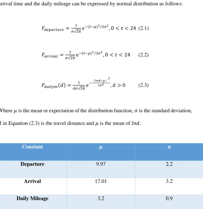
daily mileage is relevant with both departure time and arrival time. In this way, these two variables may make the probability density of the daily mileage change. The departure time, arrival time and the daily mileage can be expressed by normal distribution as follows:
𝐹𝑑𝑒𝑝𝑎𝑟𝑡𝑢𝑟𝑒= 1 𝜎√2𝜋𝑒 −(𝑡−𝜇)2/2𝜎2, 0 < 𝑡 < 24 (2.1) 𝐹𝑎𝑟𝑟𝑖𝑣𝑎𝑙 = 1 𝜎√2𝜋𝑒 −(𝑡−𝜇)2/2𝜎2, 0 < 𝑡 < 24 (2.2) 𝐹𝑑𝑎𝑖𝑙𝑦𝑚(𝑑) = 1 𝑑𝜎√2𝜋𝑒 −(𝑙𝑛𝑑−𝜇) 2 2𝜎2 , 𝑑 > 0 (2.3)
Where 𝜇 is the mean or expectation of the distribution function, 𝜎 is the standard deviation, 𝑑 in Equation (2.3) is the travel distance and 𝜇 is the mean of 𝑙𝑛𝑑.
Constant 𝝁 𝝈
Departure 9.97 2.2
Arrival 17.01 3.2
Daily Mileage 3.2 0.9
Table 2-1 Constants in distribution functions of departure time, arrival time and daily mileage.
2.2.2 Stochastic Fuzzy Model
The PHEV driving model proposed here can produce a stochastic model based on fuzzy logic. As mentioned earlier, the main task of the analog PHEV charging requirement is to
15
determine the time of insertion and insertion of the PHEV and the initial state of charge (SoC) of the PHEV. The concept of fuzzy logic can handle these three elements well. Since PHEV charging control is based on a series of time periods [5] - [13], insertion and extraction times are not always accurate. In addition, there is no need to know the exact value of the SoC. SoC can be divided into different stages, and each stage will change after charging. Different stages of the SoC can be converted to different daily driving miles. In this problem, fuzzy logic is used to classify driving patterns. The departure time, arrival time and daily mileage are divided into different ranges by the membership function. The relationship between them is defined by fuzzy rules.
The procedure of generating the driving pattern is as follows:
Step 1. According the PDFs, generate the departure time and the arrival time for a specified number of PHEVs.
Step 2. Map the input values, which generated in Step 1 to the values in the specific method.
Step 3. According to National Household Travel Survey data, generate probability matrix.
Step 4. According to random fuzzy rules, output values obtained from a probability matrix are generated and these output values are converted into clear values.
16
Step 5. Obtained the output value of the travel distance and the relative departure time and arrival time of each PHEV.
2.2.3 Initial SOC
State of charge (SoC) works as a electricity gauge for the battery pack in Electric Vehicles. The units of SoC are percentage points, while 0% indicates empty and 100% means full. In this paper, the minimum SoC is set to be 20%, which can help extend the life cycle of battery of each PHEV. PHEVs can operate in a power-consumption mode, which means that all or part of its energy can be provided by its battery.
The initial SoC of a PHEV is illustrated as follows:
𝑆𝑜𝐶𝑖𝑛𝑖𝑡𝑖𝑎𝑙= {(1 − 𝜆𝑑
𝑑𝑅) × 100%, 0 < 𝜆𝑑 < 0.8𝑑𝑅
20%, 𝜆𝑑 ≥ 0.8𝑑𝑅 (2.1)
where the 𝜆 indicates the percentage of mileage driven, d is the travel distance. It is assumed that the PHEV has an all electrical range of 𝑑𝑅.
In this way, the energy needed to charge in to the battery is:
𝐸𝑟𝑒𝑞= 1−𝑆𝑜𝐶𝑖𝑛𝑖𝑡𝑖𝑎𝑙
𝜂 × 𝐶 (2.2)
where the 𝜂 means the charging efficiency and 𝐶 indicates the capacity of battery of the PHEV.
17
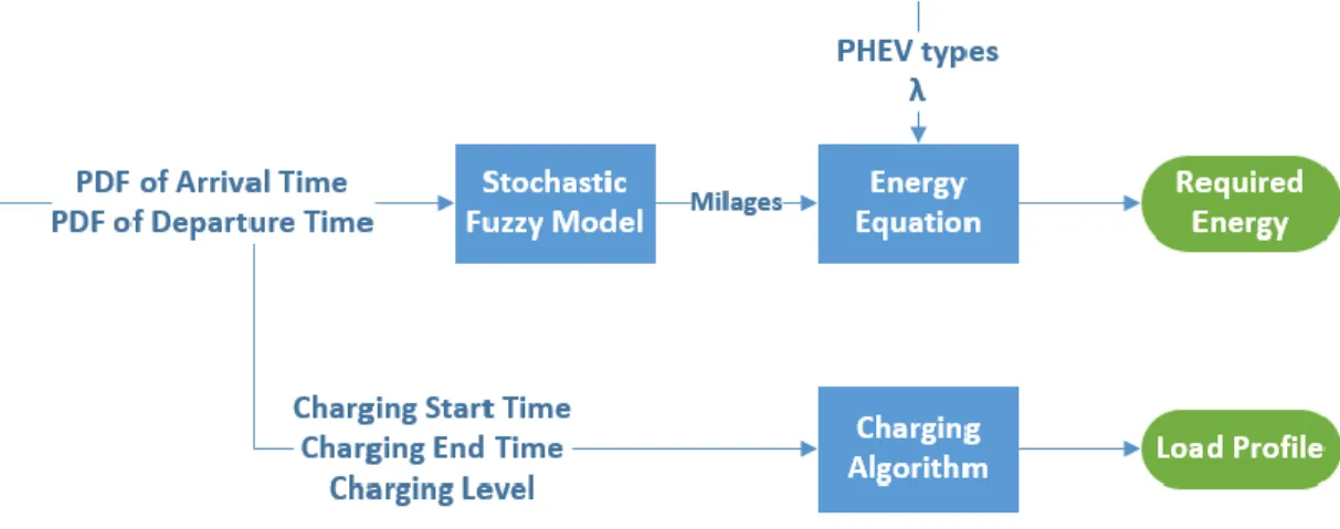
2.2.4 PHEV Load Profile
From the PHEV load profile modeling framework in Fig, the load profile can be obtained by these information and procedures. First, from the stochastic fuzzy model, the driving pattern can be generated. Next, the required energy can be generated by the combination of the daily mileage and vehicle parameters according to (2). The load profile is obtained through the required energy and its driving pattern based on a charging algorithm.
Figure 2-1 Load profile Model.
2.3 Distribution System Model
2.3.1Introduction
The distribution system in the power grid is the final step to deliver the electric power, which carries the power from the transmission system to power consumers. Primary distribution lines transmit the medium-voltage power to a distribution transformer located near the customer site. The distribution transformer again lowers the voltage to the voltage of the household appliances, and usually provide power to customers through the secondary
18 distribution line with this voltage.
Generally, the distribution system is divided into two types: (1) Ring Main Distribution System; (2) Radial Distribution System.
The ring main system is more expensive than the radial one, since there should be more conductors and switches in ring main distribution. When the generation is at low voltage, it is better to choose radial distribution system due to the low construction cost. In this way, the radial distribution system is used in this thesis.
Radial distribution system is defined as the separate feeders are radiate from a single main substation and feed the distributors at an end, which can is shown in the figure below. The power in the radial distribution is delivered from the main branch to sub-branches, and then split out from the sub-branches. As can be seen from the figure, the power is delivered from the root node, and split at L. This structure indicates that loop is not exiting in this net connection and each bus is connected to the network through one path. Due to its structure, this kind of configuration is the least reliable but the cheapest one, which is used widely in the area with less population. The radial distribution network will depart from the station and pass through the network area without any connection to other supply, especially for long rural lines in isolated load areas.
As for the node and line numbering, the nodes in radial distribution system are numbered in ascending order from lower layer to higher layer. Any path from the root node to the end node encounters nodes that are numbered in ascending order. Each branch begins with the
19
sending bus (at the root) and is identified by its unique ending bus [14].
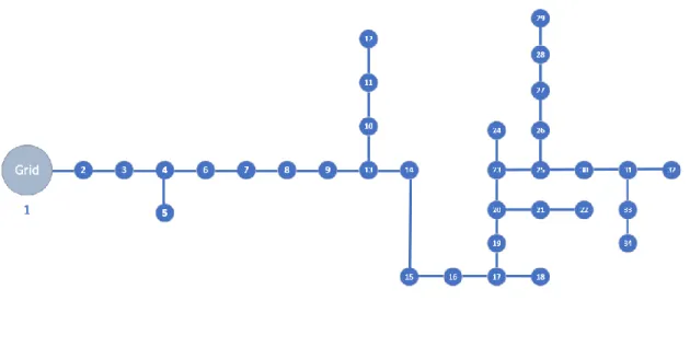
2.3.2 Residential Distribution System
The residential distribution system in this study is based on the topology of IEEE Reliability Test System (IEEE-RTS), which including IEEE 34-node test feeder [15].
In this topology, load point 1 is connecting with the power grid. There are 198 houses located in other 33 load points, which means there are 6 houses in each load point. The owner of each house has two vehicles. What is more, the penetration level can be decided as the ratio between the numbers of PHEVs and all vehicles. The non-PHEV load profile of a house is from [16]. The power flow is calculated with the backward-forward sweep method.
20
2.4 Pricing Model
Ideally the cost pay for the energy should be minimize while maintaining acceptable comfort.
2.4.1 Pricing Scenarios
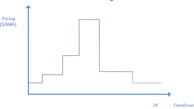
There are several different pricing scenarios addressed by the Demand Response algorithm. In this paper, there are two kinds of ricing scenarios are applied, Time-of-use(TOU) and Real Time Pricing(RTP).
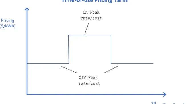
The first scenario is a Time-of-use(TOU) charge that identifies an on peak, partial peak, and off-peak time. Figure shows a scenario that has off-peak and on-peak.
21
There is a higher cost for energy use during the on-peak period, with a higher energy cost. There is also a higher charge for demand charge in additional. Demand charge is a charge related to the peak energy used. During the peak, partial peak and off-peak time periods, both the energy and de demand charge can vary. These three demand charges are typically all charged and account for the peak demand, partial peak demand and anytime demand charges. The Demand Response algorithm have to take into account the possibility for all these three kinds of charges. For Time-of-use charging strategy, it is formulated based on system load demand and can regulate the changing process. The price rate function can be defined as follow:
𝑟𝑎𝑡𝑒𝑣𝑇𝑂𝑈(𝑡) = 𝛽1+ 𝛽2𝛼
𝑃𝑠𝑦𝑠𝑡 −𝑃𝑎𝑣𝑔
𝑃𝑎𝑣𝑔 (2.1)
Where 𝛽1 and 𝛽2 are pricing parameters, and they are set to be 0.1 $/kWh and 0.2$/kWh in this paper. 𝛼 is another constant, which is 10. 𝑃𝑠𝑦𝑠𝑡 represents the load demand of the grid at time 𝑡 and 𝑃𝑎𝑣𝑔 indicates the average load demand of the grid.
Another pricing scenario that need to be addressed by the Demand Response is Real Time Pricing(RTP). The following figure shows a scenario where the pricing can change on an increment as small as 1 hour and vary quite drastically in one day. It is respected that the pricing schedule is available at the beginning of the day and available for Demand Response algorithm. If there is a change during the day. the Demand Response can operate but will not get optimally result since the future predictions are based on the characteristic
22
of this pricing scenario. The Demand Response can be able to handle the existence of an addition set of demand charges even if these demand charges may or may not be present with RTP pricing. In this paper, the real-time charging price is applied the real pricing data of one day in United States.
Figure 2-4 Time-of-use charging pricing tariff.
2.4.2 The Model of Battery Degradation Cost
The battery degradation is an economic assessment of V2G frequency regulation. The PHEVs in V2G application are considered as energy storage resource. The batteries of PHEV can use to let the power flow to the power lines from the vehicles. However, the
23
extra cost of degradation of battery is being concerned, because the current price of battery is expensive, which is more than 50% of the total cost of PHEV [17].
The equation of battery degradation cost due to V2G can be defined as follows:
𝐶𝑜𝑠𝑡𝑏𝑎𝑡𝑡𝑒𝑟𝑦 =𝑐𝑏𝐸𝑏+𝑐𝑙𝑎𝑏𝑜𝑟
𝐿𝐶𝐸𝑏𝑑𝑑𝑖𝑠 𝐸𝑑𝑖𝑠 (2.1)
where 𝑐𝑏 indicates the battery cost per kilowatt hour (kWh), 𝐸𝑏 is refined as the battery capacity, 𝑐𝑙𝑎𝑏𝑜𝑟 is the labor cost for battery replacement, 𝐿𝐶 is the battery life cycle, 𝑑𝑑𝑖𝑠
expresses the depth-of-discharge for which 𝐿𝐶 is determined, and 𝐸𝑑𝑖𝑠 is the
discharge energy by PHEVs.
2.5 Mathematics Models and Objective Function
2.5.1 Mathematics Models
In this paper, PHEVs are viewed as have three states, charging state, discharging state as well as idle state. Only when PHEVs are in idle state, it can respond to the call of frequency regulation. The equation of frequency regulation capacity can be expressed by:
𝑃𝐹𝑟𝑒𝑞𝑟𝑒𝑔𝑡 = ∑ 𝐼𝑑𝑡 𝑁
𝑑=1
∙ 𝑃𝑟𝑎𝑡𝑒𝑑 , ∀ 𝑡 ∈ 𝑇
where 𝑁 indicates the total number of PHEVs, 𝑡 means the 𝑡th time slot, 𝐼𝑑𝑡 is the idle state of the of the 𝑑th PHEV in time 𝑡, and 𝑃𝑟𝑎𝑡𝑒𝑑 is the rated charging power of the 𝑑th PHEV.
24 𝑃𝐸𝑉𝑡 = ∑ 𝑘𝑑𝑡
𝑁
𝑑=1
∙ 𝑃𝑟𝑎𝑡𝑒𝑑 , ∀ 𝑡 ∈ 𝑇
where 𝑘𝑑𝑡 indicates the charging strategy. When 𝑘 𝑑
𝑡 equals to 1, it means the 𝑑th PHEV is
in the charging state. When 𝑘𝑑𝑡 is -1, it implies the 𝑑th PHEV is discharging. As for 𝑘𝑑𝑡 is 0, the 𝑑th PHEV is in idle state.
The average load demand of the model is expressed by:
𝑃𝑎𝑣𝑔= 1 𝑇∑(𝑃𝐸𝑉 𝑡 , +𝑃 𝐵𝑎𝑠𝑒𝑡 ) 𝑇 𝑡=1 2.5.2 Objective Function
The design of objective function of this model is using the minimum cost as a figure of merit. The total cost of the system includes the charging cost, the profits of regulation service as well as the battery cost due to V2G.
The charging cost contains the charging cost and the revenue earn by discharging, which can be represented as:
𝐶𝑜𝑠𝑡𝑐ℎ𝑎𝑟 = ∑ 𝑃𝑟𝑎𝑡𝑒𝑑 𝑇
𝑡=1
∙ 𝑟(𝑡)
25
𝐶𝑜𝑠𝑡𝑟𝑒𝑔𝑢𝑙𝑎𝑡𝑖𝑜𝑛 = ∑ 𝑃𝑟𝑒𝑔𝑢𝑙𝑎𝑡𝑖𝑜𝑛𝑡 𝑇
𝑡=1
∙ 𝑟𝑒𝑔(𝑡)
where 𝑟(𝑡) indicates the electricity rate of the system and 𝑟𝑒𝑔(𝑡) is the price of regulation service in time t.
What is more, the battery cost can be defined as:
𝐶𝑜𝑠𝑡𝑏𝑎𝑡𝑡𝑒𝑟𝑦= 𝑐𝑏𝐸𝑏+ 𝑐𝑙𝑎𝑏𝑜𝑟 𝐿𝐶𝐸𝑏𝑑𝑑𝑖𝑠 𝐸𝑑𝑖𝑠
To sum up, the total power cost equation is:
𝑇𝑜𝑡𝑎𝑙𝐶𝑜𝑠𝑡 = 𝐶𝑜𝑠𝑡𝑐ℎ𝑎𝑟 − 𝐶𝑜𝑠𝑡𝑟𝑒𝑔𝑢𝑙𝑎𝑡𝑖𝑜𝑛+ 𝐶𝑜𝑠𝑡𝑏𝑎𝑡𝑡𝑒𝑟𝑦
The Objective function is:
26
Power System Reliability Analysis Methodology
3.1 Overview of Approach
To determine the minimum total cost of the system that meets series of constraints, the following steps need to use:
(1) A base vehicle platform and base vehicle characteristics are established, such as drag coefficient and accessory loads.
(2) Design parameters and constraints are selected.
(3) Relationships between the design parameters are developed based on the performance constraints.
(4) Cost functions of the design parameters are developed.
(5) Design parameters are optimized using minimum cost as a figure of merit.
3.2 Optimize Algorithms
There are many of intelligent algorithms can used to optimize a problem. Some of them are already sophisticated enough, including neural network algorithms and genetic algorithms. Particle swarm optimization and ant colony algorithms are also used widely to solve problems.
27
For the design process of these optimize algorithms, the designing of some of the algorithms are based on the observation on characteristics of society or nature. For example, neural networks, artificial fish swarm algorithms, genetic algorithms and differential evolution algorithms, belonging to the biological category. For other kind of algorithms, including particle swarm algorithm, ant colony algorithm, they belong to the category of natural science. Storm algorithm and imperial competition algorithm are obtained from sociology features.
As for the differences between algorithms whose objective functions are same, different algorithms have different benefits and drawbacks. For example, the particle swarm algorithm usually has worse convergence and it might be trapped in a local optimum easily. On the other hand, the ant colony algorithm can avoid such disadvantages. Then, a new algorithm, PSACO, can be obtained by combining the particle swarm algorithm and the ant colony algorithm together. The convergence of the PSACO is better than the convergence of a single algorithm, and it can also find the optimal result easier. However, it still depends on the goal of the optimization and the constraints on the performance of the algorithm.
3.2.1 Genetic Algorithm
Genetic Algorithm (GA) originated from computer simulations of biological systems. It is a stochastic global search and optimization method that has evolved from the biological evolution mechanism of nature. It draws on Darwin's theory of evolution and Mendel's genetic theory. Its essence is an efficient, parallel, global search method that can
28
automatically acquire and accumulate knowledge about the search space during the search process and adaptively control the search process to obtain the best solution.
The definition of concepts is listed as follow:
(1) Genotype: the internal representation of the trait chromosome;
(2) Phenotype: the external manifestation of a trait determined by a chromosome, or the external appearance of an individual formed from a genotype;
(3) Evolution: The population gradually adapts to the living environment and its quality is continuously improved. The evolution of biology takes place in the form of populations.
(4) Fitness: Measuring the adaptation of a species to its living environment.
(5) Selection: Select a number of individuals from a population with a certain probability. In general, the selection process is a process based on the fitness of the survival of the fittest.
(6) Reproduction: When a cell divides, genetic material DNA is transferred to newly created cells through replication. The new cell inherits the genes of the old cell.
29
(7) Crossover: DNA is cleaved at one and the same position on two chromosomes, and the two strings are crossed to form two new chromosomes. Also called gene recombination or hybridization;
(8) Mutation: There may be (probably a small probability) some replication errors in replication, and mutations produce new chromosomes that exhibit new traits.
(9) Coding: The genetic information in DNA is arranged in a pattern on a long chain. Genetic coding can be seen as a mapping from phenotypes to genotypes.
(10) Decoding: The mapping of genotypes to phenotypes.
(11) Individual (individual): An entity with a characteristic chromosome;
(12) Population: A collection of individuals whose number is called a population
Each chromosome in the genetic algorithm corresponds to a solution of a genetic algorithm. Generally, we use the fitness function to measure the pros and cons of this solution. So a mapping is formed from the fitness of a genome to its solution. The process of a genetic algorithm can be seen as a process of finding the optimal solution in a multivariate function. It can be imagined that there are countless “mountains” in this multi-dimensional surface, and these peaks correspond to local optimal solutions. And there will also be a “mountain peak” with the highest elevation, then this is the global optimal solution. The task of the genetic algorithm is to climb to the highest peak as much as possible instead of falling on
30
some small peaks. (In addition, it is worth noting that the genetic algorithm does not necessarily need to find the “highest mountain”. If the fitness evaluation of the problem is as small as possible, then the global optimal solution is the minimum value of the function, corresponding to what the genetic algorithm is looking for.
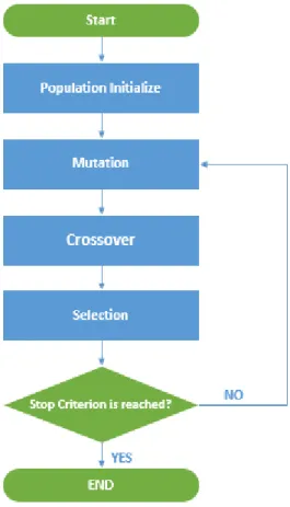
The procedures of genetic algorithm are presented as follows:
Step 1. Assess the fitness of each individual chromosome.
Step 2. The higher the degree of fitness, the greater the probability of selection, and select two individuals from the population as the parent and mother.
Step 3. Take the chromosomes of both parents and cross them to produce offspring.
Step 4. Mutate the chromosomes of the offspring.
Step 5. Repeat steps 2, 3, 4 until the new population is created. End the cycle until find a satisfactory solution.
31
Figure 3-1 The flow diagram of Genetic Algorithm.
3.2.2 Differential Evolution
The differential evolution algorithm was firstly introduced by Storn and Price in 1995. It is mainly used to solve real optimization problems, which is a kind of population-based adaptive global optimization algorithm and belongs to the evolutionary algorithm. Due to its simple structure, easy implementation, fast convergence, and strong robustness, it is widely used in mining data, digital filter design, artificial neural network, electromagnetics and other fields.
32
Similar with the genetic algorithm, the differential evolution algorithm is also an optimization algorithm based on the modern intelligence theory. It guides the direction of optimizing the search through the group intelligence generated by the mutual cooperation and competition between individuals in the group. The basic idea of the algorithm is: starting from a randomly generated initial population, a new individual is generated by summing the vector difference between any two individuals in the population and the third individual. Then comparing the new individual and the corresponding individual in the contemporary population. In the comparison, if the fitness of the new individual is better than that of the current individual, the former individual will be replaced with the new individual in the next generation. Otherwise the former individual is still preserved. By constantly evolving, retaining good individuals and eliminating inferior individuals, the optimize solution will be approached by the guidance.
The structure of it is same with genetic algorithm (GA), which can be seen from the flow chart of DE. However, it differs from the traditional GA in the process of generating new candidate solutions with using a greedy selection scheme in Mutation. The specific steps of DE is explained:
(1) Determine the differential evolution algorithm control parameters and the fitness function. The differential evolution algorithm control parameters include population size, scaling factor, and crossover probability.
33
(3) Evaluate the initial population, which means calculate the fitness value of each individual in the initial population.
(4) Determine whether the termination condition or the evolution algebra reached the maximum. If it is “Yes”, the evolution is terminated and the best individual is obtained as the optimal solution output; if it is “NO”, then continue to the following steps.
(5) Obtain intermediate populations through Mutation and Crossover operations.
(6) Select individuals in the original population and intermediate population to obtain a new generation of population.
(7) Evolutionary algebrai = i + 1, then go back to step (4).
In this paper, modified differential evolution (DE) is used to solve the power system reliability problem.
3.2.3 Particle Swarm Optimization
Particle swarm optimization (PSO) is an algorithm introduced by Kennedy and Eberhart in 1995. PSO was originally inspired by the regularity of the activities of the cluster of birds, and then a simplified model was established using swarm intelligence. PSO is based on the observation of the activities of animal groups and the use of individuals in the group to share information to make the whole group of movement in the problem-solving process space from the disorder to the order of the evolution process, to obtain the optimal solution.
34
PSO algorithm is also a kind of evolutionary algorithm. Same with the simulated annealing algorithm, it also starts from the random solution to find the optimal solution. It also evaluates the quality of the solution through fitness, but it is simpler than the genetic algorithm rules since it does not have the "crossover" and "mutation" operations of the genetic algorithm. It seeks the global optimum by following the current searched optimal value. This kind of algorithm has attracted much attention since it is easy to implement, and it has high precision, fast convergence and superiority in solving practical problems.
In PSO algorithm, the solution to each optimization problem is viewed as a bird in the specific search space, which is called by “particle”. All particles have a fitness value that is determined by the objective function. The speed of each particle determines the direction and distance they fly. Then the particle will follow the current optimal particle and search the best result in the solution space.
The initialization of PSO is a group of random particles, which is also random solutions. Then the optimal solution can be find through iterations. In each iteration, particles update the information of themselves by tracking two extreme values. The first extreme value is the optimal solution found by each particle itself. This solution is called the individual extremum, pBest. The other extremum is the optimal solution found by the entire population currently, which can be represented by the global extremum, gBest. It is also possible that to use not only the entire population, but some of them as the neighbors of the particles. Then the extremum in all the neighbors is the local extremum.
35
Figure 3_3. The flow diagram of Differential Evolution. The equations of PSO to get the best result can be expressed as:
𝑣𝑖𝑑𝑘+1= 𝑤𝑣𝑖𝑑𝑘 + 𝐶1∙ 𝑟𝑎𝑛𝑑1 ∙ (𝑝𝐵𝑒𝑠𝑡𝑖 − 𝑥𝑖𝑑𝑘) + 𝐶2 ∙ 𝑟𝑎𝑛𝑑2∙ (𝑔𝐵𝑒𝑠𝑡𝑖 − 𝑥𝑖𝑑𝑘) (3.1)
36 𝑤 = 𝑤𝑚𝑎𝑥 − 𝑘 ∙𝑤𝑚𝑎𝑥−𝑤𝑚𝑖𝑛
𝑘𝑚𝑎𝑥 (3.3)
where 𝑣𝑖𝑑𝑘is the velocity of particle at dimension, 𝑥𝑖𝑑𝑘is the position of particle along dimension, 𝑤 is the inertia weight, and 𝑘 is the iteration number.
3.3 Conclusions and Future Work
In this chapter, the methodology of optimize algorithms are introduced, especially the Differential Evolution and the Particle Swarm Optimization is discussed in details. For the future work, since optimization algorithms can combine together to get a new algorithm with better convergence or even better results, the DE or PSO can also take the advantages of other algorithms. What is more, although intelligent algorithms have been used to solve problems for a long time, it still can be improved with advanced technologies.
37
Simulation Results and Case Study
4.1 Simulation Results
4.1.1 Cost Results
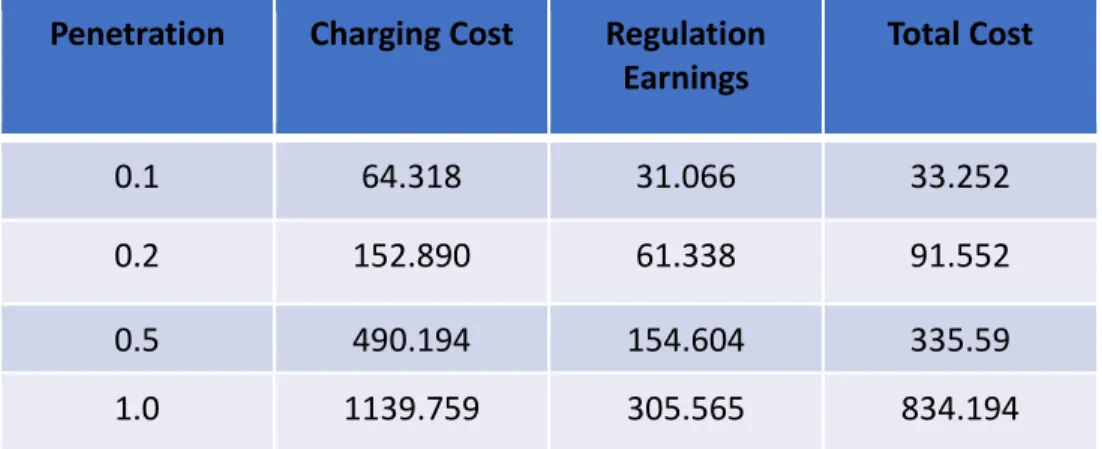
The following two tables are the economic results with Differential Evolution. It can be seen that, for the system applied Differential Evolution, with higher penetration level, the charging cost, regulation earnings and total cost will all increase. Also, the peak load is increasing with higher penetration. Similarly, the charging cost, regulation earnings as well as total cost have the same tendency of system using PSO to optimize. However, it is easy to figure out that the total cost of the DE algorithm is less than it of the PSO algorithm no matter what PHEV penetration it is. To sum up, in the economic parts, the optimization results of DE algorithm are better than these of PSO.
Penetration Charging Cost Regulation
Earnings Total Cost 0.1 60.660 31.066 29.592 0.2 145.650 61.338 84.312 0.5 465.789 154.604 311.185 1.0 1117.272 305.565 811.707
38
Penetration Charging Cost Regulation
Earnings Total Cost 0.1 64.318 31.066 33.252 0.2 152.890 61.338 91.552 0.5 490.194 154.604 335.59 1.0 1139.759 305.565 834.194
Table 4-2 Charging Cost, Regulation Earnings and Total Cost results with Particle Swarm Optimization.
Usually, only V2G technology in PHEVs is considered to provide frequency regulation services for power grid. However, PHEV has contracted with Transport System Operators through aggregators, which can provide financial incentives for PHEVs participating in regulatory services. When PHEVs provide regulatory services, the net energy exchange tends to be zero for a long time [22]. Therefore, the PHEV is paid by the power capacity provided for frequency adjustment. In this study, PHEVs are used to provide regulatory services during idle periods.
4.1.2 Load Demand of Simulations
Here are four Load demand curves of the studied system for different charging algorithms at different PHEV penetration levels, which is shown from Figure 4-1 to Figure 4-4. (a) Load demand curves at 10% PHEV penetration. (b) Load demand curves at 20% PHEV penetration. (c) Load demand curves at 50% PHEV penetration. (d) Load demand curves at 100% PHEV penetration.
39
Both the Differential Evolution and Particle Swarm Optimation can reduce the peak load. It is obvious that both of them are more effective peak load shaving at higher penetration level, since at the high PHEV penetration level, the load demand can be flatten by just shifting the charging load to valley hour. However, it is hard to figure out the large difference between the results of DE and PSO. DE is working a little bit better than PSO when the penetration level is higher.
40
Figure 4-2 Load demand curves for different charging algorithms at 20% PHEV penetration level.
41
Figure 4-4 Load demand curves for different charging algorithms at 100% PHEV penetration level.
4.1.3 Comparison of Load Voltage
Four voltage curves of node 34 for different charging algorithms at different PHEV penetration levels are shown in Figure 4-5 to Figure 4-8. They are: (a) Load voltage curves at 10% PHEV penetration. (b) Load voltage curves at 20% PHEV penetration. (c) Load voltage curves at 50% PHEV penetration. (d) Load voltage curves at 100% PHEV penetration.
42
Figure 4-5 Voltage curves of IEEE 34-node test feeder for different charging algorithms at 10% penetration level.
43
Figure 4-7 Voltage curves of IEEE 34-node test feeder for different charging algorithms at 50% penetration level.
Figure 4-8 Voltage curves of IEEE 34-node test feeder for different charging algorithms at 100% penetration level.
As shown in the figure, the proposed algorithms can reduce the voltage deviation effectively.
44
4.1.4 Peak Load
Penetration Level Peak Load of DE Peak Load of PSO
0.1 36440 36430
0.2 37140 36700
0.5 38890 38140
1.0 45170 45880
Table 4-3 Peak load of DE and PSO in different penetration levels.
4.2Case Study
V2G capacity for frequency regulation. Figure and Table 4-3 show the load demand and the cost of the system based on the three control strategies. After adding the V2G to the system, the proposed DE approach reduces the peak load, and the load demand curve becomes more flattened. V2G Technology into Simulation is more profitable for power system.
45
Figure 4-9 Load demand curves for different charging algorithms at 50% PHEV penetration level.
Table 4-4 The cost result after adding V2G into simulation.
4.2.1The total cost In Different Pricing Scenarios
There are two kind of pricing scenarios are discussed in this paper: Time-of-use pricing (TOU) and Real-time pricing (RTP).
Charging Cost Battery Cost Due to V2G Regulation Earning Total Cost Uncontrolled Charging 884.85 0 61.335 823.515 DE Charging 152.278 0 61.338 90.947 DE charging with V2G 109.524 20.724 44.678 85.570
46
The total charging cost of the system with differential evolution method is in the following table. It can be seen from the table that when the penetration is increasing, the charging cost in both pricing scenarios is getting higher. However, when the penetration level is lower to some extent, the total charging cost in TOU is less than it in RTP. When the penetration level is higher, the RTP scenario is less costly than the TOU scenarios.
Penetration Level Charging Cost in TOU($) Charging Cost in RTP($)
0.1 62.339 88.033
0.2 152.278 178.533
0.5 503.249 469.227
1.0 929.06 965.928
Table 4-5 The comparison of Time-of-use and Real-time pricing scenarios in different penetration levels.
4.3 Conclusions and Future Work
In this chapter, the optimization results of Differential Evolution and Particle Swarm Optimization as well as a group of case studies is presented. The application of V2G technology are also added into the case study.
The results show that although it hard to figure out the effectiveness of DE and PSO from the load demand curve since their curves are nearly same, the total cost of DE is smaller than the total cost of PSO. It can be concluded that DE is economic beneficial than PSO. What is more, the engineering theory and economic motivation of V2G power are convincing. What is more, the different pricing scenarios are also applied to the system to compare the different total costs under different charging price policy.
47
Conclusion
In this thesis study, a methodology for modeling the load demand of PHEVs is discussed. With this model, an economic model combined with V2G in distribution grid is developed. Two different optimization algorithms are used in this system to compare their optimization results.
This paper first introduces the basic concepts of plug-in hybrid electric vehicles, power system reliability and a series of vital concepts related to PHEVs and reliability, including vehicle-to-grid, demand response and reliability analysis methods. Then the methodology for modeling the load demand of PHEVs is introduced. Based on this stochastic PHEV model, a profit model to implement the V2G technology in a residential distribution grid is developed. In the proposed system, the PHEVs can also provide frequency regulation service and shave the peak load of the system.
The proposed thesis also implements two algorithms, namely the Differential Evolution and the Particle Swarm Optimization, to optimize the control strategies of PHEVs and achieve multiple goals by improving the power quality, reducing the peak load, providing regulation services and minimizing the total virtual cost in this system. Comparing the results at different penetration levels, a conclusion can be drawn that in most cases, the Differential Evolution offers better results compared with the Particle Swarm Optimization in terms of the minimizing the cost and the peak load of the system.
Finally, different case studies are performed under this system, including changing the penetration levels of PHEVs, implementing the V2G technology and also the charging
48
price scenarios. The results demonstrate that the overall system cost will increase with a higher penetration level. The implementation of V2G will inevitably, add some extra battery cost, however, it also provides more regulation earnings, which can definitely help improve the profits of the system. Compared to the regulation earnings, the extra cost due to V2G is much smaller. In general, the profit will be increase. Moreover, different charging scenarios lead to different cost.
There are also some future works that can be focused on later:
1. Although different penetration levels are listed and simulated in this paper, the penetration level is always under 10% in the United States due to the cheap gas price. Therefore, the best charging mechanisms in the US might be very different compared to EU or Asia. Special attention must be exercised later while examining the US scenario.
2. A thorough sensitivity study on the convergence rate and the influence from tuning the hyperparameters of the two optimization algorithms
3. Access power system reliability and cost under different models with different topologies. Consider different connections to the regional distribution network.
49
References
[1] R. Billinton and R. N. Allan, Reliability Evaluation of Power Systems. 1996.
[2] W. Kempton, J. Tomi´c, Vehicle-to-grid power implementation: from stabilizing the grid to supporting large-scale renewable energy, J. Power Sources 144 (2005) 280–294.
[3] R. Billinton, P. Wang, "Distribution System Reliability Cost/Worth Analysis Using Analytical and Sequential Simulation Techniques", IEEE Transactions on Power Systems, vol. 13, no. 4, pp. 1245-1250, Nov. 1998.
[4] “National Household Travel Survey,” 2009 [Online]. Available: http://nhts.ornl.gov
[5] P. Zhang, K. Qian, C. Zhou, B. Stewart, and D. Hepburn, “A methodology for optimization of power systems demand due to electric vehicle charging load,” IEEE Trans. Power Syst., vol. 27, no. 3, pp. 1628–1636, Aug. 2012
[6] W. Su and M. Chow, “performance evaluation of an EDA-based largescale plug-in hybrid electric vehicle charging algorithm,” IEEE Trans. Smart Grid, vol. 3, no. 1, pp. 308–315, Mar. 2012.
[7] A. Lojowska, D. Kurowicka, G. Papaehthymiou, and L. Sluis, “Stochastic modeling of power demand due to EVs using copula,” IEEE Trans. Power Syst., vol. 27, no. 4, pp. 1960–1968, Nov. 2012.
[8] T. Lee, B. Adornato, and Z. Filipi, “Synthesis of real-world driving cycles and their use for estimating PHEV energy consumption and charging opportunities: Case study for Midwest/U.S.,” IEEE Trans.Veh. Technol., vol. 60, no. 9, pp. 4153–4163, Nov. 2011.
[9] T. Lee, B. Adornato, and Z. Filipi, “Stochastic modeling for studies of real-world PHEV usage: Driving schedule and daily temporal distributions,” IEEE Trans. Veh. Technol., vol. 61, no. 4, pp. 4193–1502, May 2012.
[10]H. Sekyung,H. Soohee, andK. Sezaki, “Development of an optimal vehicle-to-grid aggregator for frequency regulation,” IEEE Trans. Smart Grid, vol. 1, no. 1, pp. 65–72, Jun. 2010.
[11]H. Liang, B. Choi,W. Zhuang, and X. Shen, “Towards optimal energy store-carry-and-deliver for PHEVs via V2G system,” in Proc. IEEE INFOCOM, Mar. 2012, pp. 1674–1682.
[12] B. Lunz, H. Walz, and D. U. Sauer, ““Optimizing vehicle-to-grid charging strategies using genetic algorithms under the consideration of battery aging,” in Proc. IEEE Veh. Power Propuls. Conf. (VPPC), Sep. 2011, pp. 1–7.
[13]S. Han, S. Han, and K. Sezaki, “Economic assessment on V2G frequency regulation regarding the battery degradation,” in Proc. IEEE PES Innovative Smart Grid Technol. (ISGT), Jan. 2012, pp. 1–6.
[14]Bompard, E. Carpaneto,” Convergence of the backward/forward sweep method for the load-flow analysis of radial distribution systems” Electrical Power and Energy Systems 22 (2000) 521–530. [15] W. H Kersting, “Radial distribution test feeders,” in Proc. IEEE Power Eng. Soc. Winter Meeting, Jan.
2001 [Online]. Available: http://ewh.ieee.org/soc/pes/dsacom
[16][J. A. Jardini, C. M. Tahan, and M. R. Gouvea, “Daily load profiles for residential, commercial and industrial low voltage consumers,” [IEEE Trans. Power Del., vol. 15, no. 1, pp. 375–380, Jan. 2000. [17][W. Kempton and J. Tomic, “Vehicle-to-grid power fundamentals: Calculation capacity and net revenue,”
J. Power Source, vol. 144, pp.268–279, 2005.]
[18]W. Kempton and J. Tomic, “Vehicle-to-grid power fundamentals: Calculation capacity and net revenue,” J. Power Source, vol. 144, pp. 268–279, 2005.
50
[19]W. H Kersting, “Radial distribution test feeders,” in Proc. IEEE Power Eng. Soc. Winter Meeting, Jan. 2001 [Online]. Available: http://ewh.ieee.org/soc/pes/dsacom/
[20]J. Kennedy and R. C. Eberhart, “Particle swarm optimization,” in IEEE Int. Conf. Neutral Netw., 1995, pp. 1942–1948.
[21] S. Hadley, “Impact of plug-in hybrid vehicles on the electric grid,” Oak Ridge National Lab., Oak Ridge, TN, USA, Tech. Rep. ORNL/TM-2006/554, 2006.
[22] W. Su, H. Eichi, W. Zeng, and M. Chow, “A survey on the electrification of transportation in a smart grid environment,” IEEE Trans. Ind. Informatics, vol. 8, no. 1, pp. 1–10, Feb. 2012.
![Figure 1-1 Hierarchical Levels of Power System [1].](https://thumb-us.123doks.com/thumbv2/123dok_us/1226710.2665221/14.918.261.696.746.1038/figure-hierarchical-levels-power.webp)
![Figure 1-3 Schematic of control connections between PHEVs and power grid [2].](https://thumb-us.123doks.com/thumbv2/123dok_us/1226710.2665221/18.918.233.752.276.569/figure-schematic-control-connections-phevs-power-grid.webp)