WORKING PAPER 07-2
Jeremy T. Fox and Valérie Smeets
Do Input Quality and Structural Productivity
Estimates Drive Measured Differences in Firm
Productivity?
Department of Economics
ISBN 87-7882-193-2 (print) ISBN 87-7882-194-0 (online)
Do Input Quality and Structural Productivity Estimates Drive
Measured Differences in Firm Productivity?
Jeremy T. Fox & Valérie Smeets
∗University of Chicago
Universidad Carlos III & CCP
February 2007
Abstract
Firms in the same industry can differ in measured total factor productivity (TFP) by multiples of 3. Griliches (1957) suggests one explanation: the quality of inputs differs across firms. Labor inputs are traditionally measured only as the number of workers. We investigate whether adjusting for the quality of labor inputs substantially decreases measured TFP dispersion. We add labor market history variables such as experience and firm and industry tenure, as well as general human capital measures such as schooling and sex. We also investigate whether an innovative structural estimator for productivity due to Olley and Pakes (1996) substan-tially decreases measured residual TFP. Combining labor quality and structural estimates of productivity, the one standard deviation difference in residual TFPs in manufacturing drops from 0.70 to 0.67 multiples. Nei-ther the structural productivity measure nor detailed input quality measures explain the very large measured residual TFP dispersion, despite statistically precise coefficient estimates.
JEL codes: D24, L23, M11
Keywords: production function estimation, total factor productivity, input quality, structural estimates of pro-ductivity
Abstract
∗Thanks to helpful discussions with Daniel Ackerberg, Ulrich Doraszelski, Tor Eriksson, Amil Petrin, Chad Syverson and Frédéric
Warzynski. Thanks to the professional staff at CCP, Aarhus School of Business, for hospitality and for help integrating the KØB and IDA datasets. Our email addresses are [email protected] and [email protected].
1
Introduction
Differences in output across firms can be decomposed into differences in measured inputs and differences in residuals. The literature typically estimates the Cobb-Douglas production function
y=β0+βll+βkk+e, (1)
whereyis the log of value added,l is the log of the number of workers, andkis the log of the dollar value of physical capital. βl andβkare the input elasticities of labor and capital. Between two firms with the same inputsl andk, the firm with the higher outputyis said to have a higher measured total factor productivity (TFP), which is exp(β0+e)above.
Measured differences in productivity across plants in the same industry can be large. Bartelsman and Doms (2000) survey the literature and find many instances where the highest productivity firm has more than twice the measured productivity of the lowest productivity firm. Also, Dhrymes (1995) studies American manufacturing firms and finds that the ratio of TFP of plants in the ninth decile to the TFP of plans in the second decile is 2.75 in 1987. We find that the standard deviation of log TFP is 0.54 in manufacturing, in Denmark. The TFP level of two standard deviation differences is exp(2·0.54)−1=1.94 multiples.
These huge differences in cross-sectional, measured TFPs have spawned a literature investigating why produc-tivity differences are so large. One explanation is simply measurement error: eis dominated by noise added to the dependent variable, outputy. However, measured productivityeis persistent across time, meaning any measurement error cannot be transient (Baily, Hulten and Campbell, 1992). Managerial competence or overall business strategies are another major explanation (Bloom and Van Reenen, 2007). A well run business will produce more from the same inputs. Business strategy is likely to play even more of a role when one considers that the dependent variable in a productivity regressionyis typically firm sales or value added, and the pricing decision of a firm affects sales (Foster, Haltiwanger and Syverson, 2005). Also, firms likely use technologies of varying qualities due to previous R&D decisions (Doraszelski and Jaumandreu, 2006).
Economists since at least Griliches (1957) have put forward another hypothesis: the quality of inputsl and
kvaries across firms. Economists working with US manufacturing plant data typically measure inputs as the dollar value of physical capital and the number of workers at a firm. At best, employees are separated into production and nonproduction workers. Not surprisingly, labor and capital vary in much greater detail. Two types of machines may have different uses and may not be perfect substitutes, and two types of workers may not have the same contributions to firm output. Our first contribution is to disaggregate the labor input. We use matched employer-employee data from Denmark to precisely measure many characteristics of workers at a firm. Schooling, sex, total experience and industry tenure proxy for general or occupation-specific human capital inputs. Tenure at a worker’s current firm proxies for firm-specific human capital.
firm-level measures of individual worker characteristics into efficiency units of labor. This labor quality function is embedded in the estimation of an otherwise standard Cobb-Douglas production function. The residual from this production function estimate is a firm’s total factor productivity (TFP). We examine whether adjusting for labor input quality reduces the measured within-industry dispersion in residual TFP (RTFP), or the standard deviation ofe. As RTFP is just a residual, we examine to what degree do labor input quality measures increase the fit to output data. Fit is measured byR2=1−Var(e)
Var(y).
Standard models predict that more productive firms use more inputs. If true TFP is correlated with inputs, then our production function estimates will be biased and our residualsewill not consistently estimate a firm’s true TFP. Griliches and Mairesse (1998) suggest that panel data approaches are very sensitive to measurement error. Consequently, we use cross-sectional variation to correct for the potential correlation of inputs with the unmeasured TFP term. We parametrize the intercept (mean TFP) with observable characteristics such as firm age and recent firm growth that are likely correlated with TFP. Also, we adopt (the simultaneity part of) a strategy inspired by Olley and Pakes (1996). Conditional on a firm’s non-TFP state variables, its physical capital and firm age, under some modeling assumptions a firm’s investment provides a proxy for its productivity. We add a polynomial in capital, investment and firm age in order to proxy for a firm’s unobserved TFP.1 The Olley and Pakes (henceforth OP) procedure produces a direct, structural estimate of TFP. In other words, the OP procedure decomposes composite error termse=ω+ηintoω, structural TFP, andη, measurement error. Our second contribution is to examine to what degree this structural estimate of productivityωexplains measured dispersion in RTFP, ore.
OP is typically used to correct estimates of input elasticitiesβkandβlfor the correlation of inputs withω. The structural estimates ofωare not of primary interest if input elasticities are the objects of interest. However, much of the productivity literature focuses on the puzzle that the cross-sectional dispersion in measured RTFP is so large. To this end, the direct, structural estimates of TFPωin OP have the potential to solve the RTFP puzzle.
We show that, consistent with the US manufacturing plant evidence, there is large degree of measured RTFP dispersion across Danish firms. With only the number of workers and the dollar value of capital as inputs, we find that a firm with one standard deviations more log RTFP has in RTFP levels exp(0.54)−1=0.72 times more output for the same inputs, in manufacturing. For three other sectors, our measured TFP dispersion is even higher.
Note that from now on, we automatically translate the standard deviation of log RTFP into RTFP levels by the function exp(sd(log RTFP))−1.2 This reports the difference in multiples in RTFP for firms one standard deviation of log RTFP away. We defineσ=exp(sd(log x))−1, wherexis typically RTFP and the units ofσ are in multiples. One standard deviation is conservative; exp(2·sd(log RTFP))−1 is a much bigger number.
1See Van Biesebroeck (2007a) for a comparison of OP to other simultaneity-correction methods. 2The standard deviation of log RTFP is related toR2by the formula sd(log RTFP) =q 1−R2
We find that human capital inputs are correlated with firm value added. In other words, the coefficients on our labor quality measures have economically large magnitudes that are typically statistically distinguishable from zero.
However, the magnitude of the decrease in RTFP dispersion from including labor quality measures is small, for most sectors. For manufacturing,σdrops from 0.72 to 0.68 multiples.
Finally, we find that the Olley and Pakes (1996) structural TFP dropsσhardly at all in manufacturing:σstays at 0.70 multiples. Adding the OP structural productivity termωdoes not increase the statistical fit, R2, of log-productivity regressions (∆R2=0.002), even if input elasticities are precisely estimated in large samples. Combining labor quality and the structural estimation of true productivityω, we find thatσdrops from 0.70 to 0.67 multiples.
The estimates show that the OP structural TFPωhas aσfor true TFP of 0.12 multiples. As above, the OP RTFPσexcludingωis 0.70 multiples, much higher than 0.12. The OP structural interpretation of the original, non-OP measured, residual TFP dispersion is that it is dominated by measurement error. Another interpretation consistent with OP is thatηrepresents contributions to productivity that occur after investment decisions are made.
The OP structural interpretation ofηas measurement error conflicts with the literature’s view that as RTFP is autocorrelated at the plant and firm levels, RTFP dispersion is not caused by classical, independent across time measurement error (Baily et al., 1992). Any measurement error is time persistent. We find that the year 2000 OP measurement error has a correlation of 0.80 with the same-firm year 2001 OP measurement error, in manufacturing. Thus,ηis less likely to represent innovations in productivity after investment decisions are made.
Our results have several implications for production function estimation. First, inferences about across-firm RTFP dispersion are not sensitive to measurement error in input quality. For many research questions, using the number of workers rather than more detailed input measures will suffice. Second, including the OP structural measureωdoes not reduce RTFP dispersion by a large magnitude. In terms of statistical fit, adding investment to a productivity regression explains little of the RTFP dispersion.
Third, the high autocorrelation in OP’s structural measurement errorηsuggests the possibility that not all of this term is really measurement error. In terms of statistical fit, again this suggests thatωdoes not capture all differences in productivity across firms.
Fourth, in terms of consistent estimation of the input elasticities (omitted variable bias), the high autocorrelation inηis a violation of a maintained assumption of OP, unlessηis not used to make input decisions by firms. The typical concern with endogeneity is that more productive firms use more inputs. OP’s theoretical inversion procedure investment to be monotone in a scalar unobservable. A firm may have multiple unobservables such
as demand shocks and input price shocks.3 With multiple unobservables, OP is not a consistent estimator of
input elasticities,ωandη. Even if the trueηis measurement error, the accounting reports with measurement error could be forwarded to executives and used to make decisions. If firms use the trueη to make input decisions, then OP will not be consistent for the input elasticities,ωandη.
Overall, our results show that the high cross-sectional dispersion in measured productivities is not explained by input qualities and the most commonly used structural productivity estimator. For measuring productivity, we find evidence against the reasonable conjecture by (Griliches, 1957) that a large part of productivity dispersion comes from mismeasured inputs. We return to this point in our conclusion.
The original paper by Olley and Pakes (1996) has inspired many methodological advances, such as Levinsohn and Petrin (2003) and Ackerberg, Caves and Frazer (2007).4As Ackerberg et al. argue, the consistency of OP and related methods rely on the ability to decomposeeintoωandη. Still, none of these papers report statistics on the decomposition ofeinto the structural TFPωand measurement errorηcomponents. OP work witheas a composite error term.5Using the composite residualerather than the structural decomposition allows
compar-isons between RTFP in studies using OP and other studies. However, the structural interpretation is necessary to understand whether OP explains the large measured RTFP dispersions with structural measurement error or true productivity.
Several recent papers combine worker and output data, either to compare the production and wage regression coefficients (Van Biesebroeck, 2007b) or to control for worker ability in wage regressions (Frazer, 2006). We are focused on firm productivities and do not consider wages. The statistical fit labor input quality aspect of our work is similar to Hellerstein and Neumark (2006), who also find a low reduction in RTFP when adding labor quality measures using US manufacturing data. The magnitudes of the RTFP dispersion reduction are hard to compare between the two papers because Hellerstein and Neumark include materials as an input (which raisesR2), while our measure of output is value added. We also use labor history measures (experience, industry tenure and firm tenure) constructed from 21 years of panel data for all Danish citizens, and include four industry sectors, of which only one is manufacturing.
3For example, a firm may produce products with a limited market, meaning that advances in productivity do not encourage the firm to
expand its output.
4See Doraszelski and Jaumandreu (2006) for another approach that uses a parametric first order condition for labor demand rather than
a nonparametric control function.
5OP discuss this decision in their footnote 33 on page 1287. In their empirical application, OP focus on same-plant TFP growth, not
2
Production functions
2.1
Overview
A production function takes inputs and produces outputs. Our measure of output is a firm’s value added, which is just total sales minus materials and other outsourced inputs, such as consulting services. Subtracting materials from sales is valid if materials and other inputs combine using a Leontief production function. At least in manufacturing, a fixed-proportions materials technology is realistic as a given product often requires particular ingredients.6
The “total factor” in TFP refers to including two inputs, labor and capital. The residualeis, without structural interpretation, the output residual and hence the residual to log measured TFP. Total measured log TFP isβ0+e,
so the variance ofeis the variance in residual TFP, or RTFP. The puzzle we seek to explain is why the estimated standard deviation of the residualeacross plants, measured RTFP dispersion, is so high. AsR2=1−VarVar((ey)), we wonder why the statistical fit of log-valued added production functions is so poor.
2.2
Labor quality
We first investigate one explanation for the lowR2and consequently high dispersion in measured RTFP: quality differences in labor inputs. As workers with more schooling and experience are paid higher wages, it would not be surprising to find that those workers contribute more to output. If one can only measure the total number of workersl, then the deviation between the true and measured efficiency units of labor will enter the error term and increase measured TFP dispersion, while at the same time causing an estimation bias due to measurement error.
Following a suggestion by Griliches (1957), we view the labor input as the number of workers times labor quality. Each worker is a bundle of measured characteristics. We unbundle workers so that labor quality is a function of the fraction of workers in a firm with each characteristic. In a firm with 100 workers, hiring 1 more woman with a college degree will increase the fraction of workers who are women by 1% and the fraction of workers with college degrees by 1%. Letxfemale be the fraction of workers who are women, andxcollegethe
fraction with a college degree. Total labor quality has the multiplicative functional form
qθ(x) = (1+θfemalexfemale) 1+θcollegexcollege. (2)
Here, efficiency units of labor are measured in some base units: the relative productivity compared to a male high-school graduate, say. In this case,θfemale is how much more productive a woman is relative to a man,
6While not reported, our conclusions about RTFP dispersion are robust to estimating a CES instead of Cobb-Douglas production
andθcollegeis how much more productive a college educated worker is relative to a worker who did not attend
college. A firm of all men where 100% of its workers attend college will have a per-worker quality of 1+ θcollege. Note that a multiplicative labor quality measure is also used in Hellerstein and Neumark (2006).
Labor quality is not additively separable across workers, as in Welch (1969). For example, expanding the specification ofqθ(x)above produces the interaction termθfemalexfemaleθcollegexcollege. If theθ’s are positive, adding a male college graduate will produce a greater increase in labor quality at a firm with more women. Let the total number of workers at a firm ben. The total labor input is thenl=n·qθ(x). Substituting this
expression forlin the Cobb-Douglas production function (1) gives the estimating equation
y=β0+βln·qθ(x) +βkk+e.
The parametersθenter this equation nonlinearly, so estimation is by nonlinear least squares. It would be ideal to also measure the quality of physical capital,k. Our accounting data do not allow us to measure physical capital in other than monetary terms.
2.3
Olley and Pakes (1996)
Both true TFPωand measurement error ηcause unmeasured variation iny, so, following Olley and Pakes (1996), we sete=ω+η. Marschak and Andrews (1944) introduced the concern that Cov(l,ω)>0 and Cov(k,ω)>0, or that more productive firms systematically use more inputs. This leads to a standard endo-geneity problem, where the contributions from productivity are misattributed to inputs.
One solution is to parametrize mean log TFP,β0, as a function of observable firm characteristics such as firm
age and recent firm growth. If these variables partially proxy forω, then the remaining ˜ωwill be less correlated with the measured inputs. Also, the measurement errorη will play a larger role in the new ˜e, as previous components ofωare captured by observables.
Our other approach to dealing with the cross-sectional correlation of inputs and TFP residuals is inspired by Olley and Pakes (1996) or OP.7Following OP, we estimate the Cobb-Douglas production with firm age included
as a measurable component of TFP:
y=β0+βaa+βll+βkk+ω+η.
OP use a theoretical model of a forward-looking firm where capital is slowly accumulated. Leti represent investment. OP’s model shows that, between two firms with the same physical capitalkand agea, the firm 7Ackerberg et al. points out inconsistencies in the arguments of Olley and Pakes and Levinsohn and Petrin. There is an alternative set
with the higher TFP invests more:
i1>i2ifk1=k2,a1=a2andω1>ω2. (3)
If there is no measurement error in inputs, one can use a nonparametric functionφ(i,k,a)of investment and capital to proxy for the contributions of non-age TFP and the direct contributions of the inputsaandk. Ac-cording to OP’s model,
φ(i,k,a)−βkk−βaa−β0=ω,
and so an estimate ofφ(i,k,a)−βkk−βaa−β0is an estimate ofω. This point is important:φ(i,k,a)is not only a control function to correct for the simultaneity bias,φ(i,k,a)−βkk−βaa−β0equals the structural TFP
ω, according to OP’s model.
We implement the simultaneity portion of OP in two steps:
1. Regressyonlandφ(i,k,a)to estimateβl, and the labor quality variables when included. TheR2from this step is the total explanatory power of inputs and structural productivity: βll,βkkandω. ThisR2is one of our main focuses.
2. Regressy−βˆll ona,kand a polynomial in the term ˆφ(i,k,a)−βaat−1−βkkt−1, wheret−1 refers to
the year 2000 instead of 2001. Nonlinear least squared must be used asβaandβkenter the polynomial nonlinearly. This step is motivated by a panel data moment condition.
We estimate separately for four sectors, so we can control as best as possible for unmeasured input prices entering the inversionφ. To address whether our results arise from pooling too many heterogeneous industries, we also list separate results for a manufacturing industry with a large number of firms.
We produce estimates for the year 2001, although the second stage also uses firm-level data from 2000. We do not implement OP’s selection-correction procedure for endogeneous entry and exit. Our primary goal is to structurally estimateωand identify the magnitude of its cross-sectional variation across firms. We treat the estimatedωas an observable and add its contribution toR2.
We conjecture that tweaks to the procedure will not cause dramatic increases in theR2of the first stage, which comes from adding a polynomial ina,kandito a standard Cobb-Douglas production function. Ignoring non-linearities, we measure whether adding investment and firm age to a production function noticeably increases
R2. To preview, we find that it does not.
2.4
Labor as a dynamic choice variable
OP relies on the idea that labor is a static choice variable. Given that we find a positive correlation between value added and inputs such as workers’ tenure at a firm, the labor input is likely to be chosen with regard to
last period’s stock of labor. This is a problem with the OP structural interpretation ofωas true productivity, but not the facts aboutR2, which are purely about data fit.
Ackerberg, Caves and Frazer (2007) modify OP to treat labor and physical capital symmetrically: labor can be a dynamic input. In a first stage, one regresses outputyonφ(i,k,l,a), a polynomial in investment, capital, labor and firm age. TheR2from this regression is the total explanatory power of inputs and structural productivity ω. In unreported results, we implement this procedure by adding labor to the polynomial. Not surprisingly,R2
goes up very little.
3
Danish labor and accounting data
We need data on a firm’s inputs and its output as well as measures of labor quality to estimate the impact of labor quality variables in the production function.
We use accounting data for capital, value added and investment. The accounting data come from Købman-standens Oplysningsbureau (KØB), a Danish credit rating agency. The accounting data are an unbalanced panel that roughly covers the period 1995-2003 and use each firm’s proprietary accounting period. We rescale the accounting variables to a twelve-month, calendar year basis. The accounting data were designed foremost to provide financial information for firms currently operating in 2003. We look at the year 2001 to maximize the number of firms with complete calendar year data. The OP second stage uses 2000 data, and we inflate 2000 monetary values to 2001 units.
We use value added as a measure of output and fixed assets for capital. Value added is reported for many more firms that total sales, perhaps because of the role of value added in value added taxes. We disregard firms who do not have rescaled accounting information on valued added and fixed assets for a 12 months period. For the labor input, we count the total number of workers in IDA, which is described below.
Firm age is directly reported in the accounting data. We include the log of firm age in some specifications. We construct investment from the accounting data in order to estimate true TFPωusing the OP approach. Investment is computed using the formulai=k2001−(1−δ)k2000, whereδis the depreciation rate. Investment
cannot be missing and firms must be present in both 2000 and 2001. The accounting data report δk2000,
which we use to back outδ. We experimented with the Levinsohn and Petrin (2003) procedure to proxy for productivity using capital and materials inputs. We defined materials as total sales minus value added. However, we have data on total sales and hence materials for a small sample of firms. As this sample is highly selected, we do not report the Levinsohn and Petrin estimates.
To construct labor quality variables, we use the Danish Integrated Database for Labor Market Research (IDA), one of the central registers of Statistics Denmark. IDA integrates three types of data. The first dataset provides information at the individual level on demographics (age, sex, martial status, family status) and schooling for
all Danish citizens over 1980–2001. Each individual is given a unique identification number that can be further used for matching with the other datasets of IDA. The second dataset of IDA is at the level of an individual’s job. It contains information on individual labor earnings and labor market variables and the number of years of labor market experience. Labor market experience is computed since 1964.
Both full and part time jobs are included, but in the rare case of a worker with three or more jobs, only the primary and secondary jobs are reported. The data also contain a unique identification number for each job’s establishment. IDA’s establishment data provide a firm identification number that can be use for matching with other firm-level data.
We use IDA for 1980–2001 to compute labor market history variables such as firm tenure and industry tenure. Experience is calculated by Statistics Denmark. We compute firm tenure as the number of years a worker has been attached to a given firm. As we are concerned with spurious changes in firm identification codes over time, a worker’s tenure is reset to zero only if both his firm and establishment identifiers change at the same time. We construct industry tenure using the following eight industry sectors: (1) agriculture and mining, (2) manufacturing, (3) construction and transport, (4) retail, hotels and restaurants, (5) finance, real estate and R&D activities, (6) public sector, (7) private households and extraterritorial activities and (8) others.
Industry is recorded at the establishment level. For our regressions, a multi-establishment firm’s industry is the weighted (by number of workers) modal establishment industry.
All inputs are constructed at the firm level. We construct firm-level fractions of workers who have a given characteristic, say a college degree or 6–9 years of firm tenure. The intervals are simple to interpret as each measure is a fraction between 0 and 1. The intervals allow us to examine nonlinearities across the intervals, and they handle topcoding from not observing firm and industry tenure for spells starting before 1980. We then match the firm characteristics to the accounting data using the firm identification numbers provided by Statistics Denmark.
We estimated production functions for two samples: all firms with nonmissing variables and a sample with outliers removed. We are worried about possibly non-classical measurement in the accounting data, so we removed the firms in the top and bottom 1% of output to labor and physical capital to labor ratios. Removing these outliers increases the baseR2’s substantially, but does not change the∆R2’s from labor quality and OP much at all. We report specifications with the outliers removed, but our main conclusions about∆R2’s are similar if we include the outliers.
4
Sample statistics by sectors
We only consider private-sector firms that have at least ten employees. We group lower-level industries into four sectors: (i) manufacturing, (ii) construction and transportation, (iii) retail, hotels and restaurants and (iv)
finance, real estate and R&D activities. Unfortunately, Denmark is a small country and there are few firms in each more narrowly defined industry, although we sometimes include lower-level industry fixed effects. To see whether pooling industries affecting our results, we also separately estimate production functions for a manufacturing industry with a large number of Danish firms: machinery & equipment. We look at a cross section of firms in the year 2001.
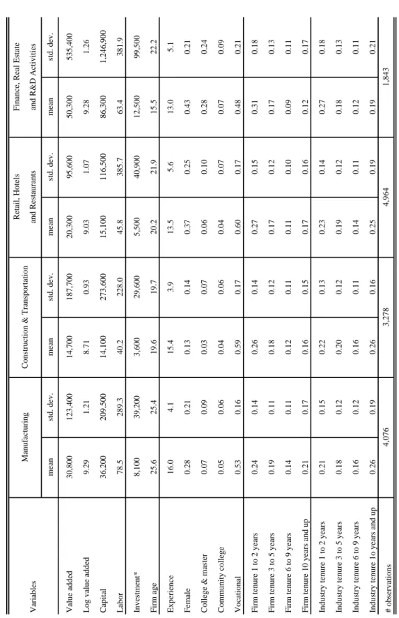
Table 1 lists summary statistics for each large sector. The second line documents our dependent variable: the standard deviation in log value-added. The standard deviation of log value added in manufacturing is 1.21, meaning that a 1-standard deviation higher log value added corresponds to aσof exp(1.21)−1=2.35 multiples in value added.
Finance is the most (measured) capital intensive sector and retail and construction are the least. Manufacturing has the most workers per firm at 79, and construction the least with 40. Recall we consider only firms with ten or more workers.
The other summary statistics report information on workforce composition. The fraction of female workers is the highest in finance and retail and the lowest in manufacturing. The finance sector has the most highly edu-cated workforces. Workforces in manufacturing and construction have the highest experience levels. Finally, workforces in finance have lower firm and industry tenure than other industries’ workers.
The standard deviations of the human capital inputs show that there is a reasonable amount of variation in the characteristics of workforces within each sector. Many standard deviations are similar in magnitude to the means themselves. Finance has the highest standard deviations, followed by retail, construction and finally manufacturing. The standard deviations are important, because any reduction in TFP dispersion (an increase in
R2) comes from both variation in workforce composition across firms as well as the estimated parameters on the labor quality measures.
5
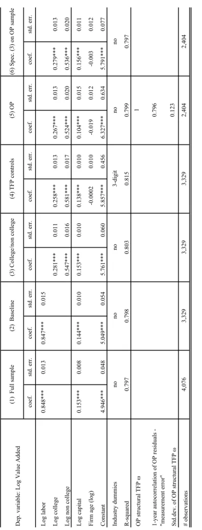
Production function estimates w/o labor quality
Table 2A reports estimates of production functions such as (1) for the manufacturing sector. The first column uses all observations with nonmissing value added and capital, while the second column uses only observations with positive numbers of both college and noncollege workers. The college sample is then used to break out the number of workers into college and noncollege (third column) and then to add firm observables that could proxy for TFP, such as the log of firm age (fourth column) and three digit industry dummies. In an unreported specification, we add a five year growth measure due to Davis and Haltiwanger (1992). Compared to the baseline in the second column,R2increases from 0.798 to 0.803 from breaking labor inputs into college and noncollege, and from 0.803 to 0.815 from adding firm age and the full set of three-digit industry dummies. Firm age, schooling and industry heterogeneity in mean TFP are not the keys to understanding cross-sectional
dispersion in RTFP. With aR2of 0.815, VarVar((ey))=0.185, so measured RTFP comprises 19% of the variation in log output across firms.
As an aside, the sum of the coefficients on the numbers of college and noncollege workers in third column is only 0.019 different from the coefficient on the total number of workers in the second column. Also, while we do not impose constant returns to scale, an estimate very close to it always appears.
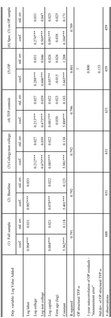
The fifth column of Table 2A reports estimates using the simultaneity-correction procedure of Olley and Pakes (1996), as discussed in Section 2.3. The estimation uses a reduced sample because of missing investment data. Investment data are needed for both 2000 and 2001 because of the OP second stage. For comparison, the sixth column contains an OLS specification on the sample of manufacturing firms with nonmissing investment. The estimates in the sixth column are not identical to but look similar to those in the third column with the larger college sample. Therefore, we suspect the missing investment data do not dramatically alter our results. The OP procedure changes the point estimates only a little. Also, theR2 increases by only 0.002 when we structurally estimateω, the true TFP in OP, and includeωas a regressor (coefficient is 1) that contributes toR2. Later we will directly calculate the standard deviation of log RTFP. For now, it appears that OP will not reduce measured RTFP a lot. The estimated standard deviation ofωis 0.12. This is not small, but aσof 0.12 (12%) is smaller than theσof 0.70 for OLS applied to the OP estimation sample and theσof 0.70 for the measurement error in the OP estimates. The later numbers appear in Table 7; we will discuss them soon.
One question is whether the structural measurement errorηis i.i.d. over time. Table 2A shows it is not: the same-firm correlation betweenηin 2000 and 2001 is 0.80.
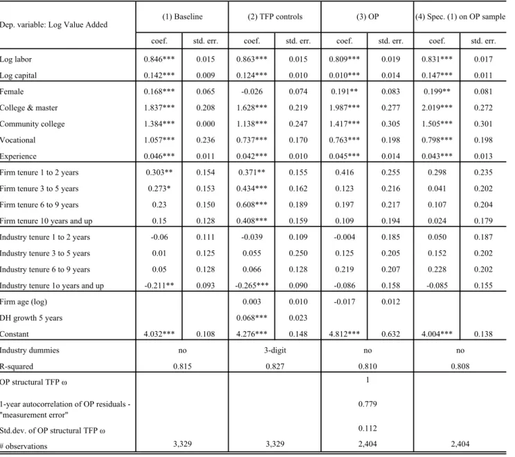
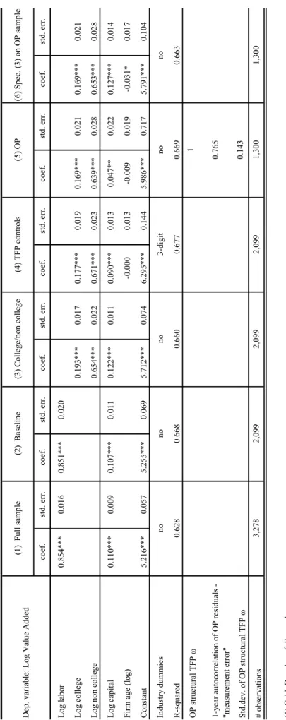
Tables 3A, 4A and 5A repeat the above analysis for construction, retail and finance, respectively. The base coefficient estimates and the base R2’s vary across sectors. R2’s are lower in the three sectors other than manufacturing. This likely reflects the greater heterogeneity in technology in these sectors. Below we use a narrower industry grouping to better control for heterogeneous technologies.
Disaggregating college graduates from other workers increasesR2(compare columns (2) and (3) in Tables 3A, 4A and 5A) by -0.008 in construction, a large 0.056 in retail and 0.004 in finance.
Adding firm age and industry indicators increasesR2by 0.017 in construction, 0.051 in retail, and 0.051 in finance. While not large compared to the 35% of log value added variance explained by residuals, these can be considered large∆R2’s reflecting measured differences in log TFPs.
Comparing columns (6) and (5) in Tables 3A, 4A and 5A gives changes inR2due to the OP procedure of 0.006 in construction, 0.011 in retail, and 0.018 in finance. These are relatively small∆R2’s compared to the typically 35% of log value added variance explained by measurement error in the structural OP interpretation. Again, these results will be explained in more detail soon.
As for the input elasticities, the OP procedure noticeably decreases the coefficient on physical capital in con-struction (Table 3A) and finance (Table 5A). An upward bias is predicted by the univariate OLS endogeneity
bias formula when more productive firms use more capital, so the effects of unmeasured productivity (the error term) are falsely attributed to the inputs in OLS. However, the typical suspicion in the literature is that capital coefficients are underestimated. Note that the OP estimate of the capital coefficient comes from a panel data moment condition, not just including investment as a regressor.
Our industrial sectors cover much more than the typical manufacturing industries studies in the productivity literature. However, our sectors do pool potentially heterogeneous industries because of the limited size of Denmark. To address pooling, Table 6A considers a narrower manufacturing industry with a large number of firms: machinery and equipment. Compared to all manufacturing firms in Table 2A, the results for machinery show that OP increasesR2by 0.012, while adding TFP controls increasesR2by only 0.004. In a more disag-gregated sector, the relative∆R2’s of OP and TFP controls are reversed, but the bottom line remains that both ∆R2’s are small.
6
Production function estimates with labor quality
6.1
Statistical fit
Tables 2B, 3B, 4B and 5B report estimates of production functions with labor quality measures. The functional form for labor quality is equation (2).
Look at column 1 in Table 2B, for manufacturing. This uses the same sample as column 2 in Table 2A. We see that adding the labor quality measures increasesR2from 0.798 or 0.815, so∆R2=0.017. In column 2 of 2B, adding firm age, five year growth according to a Davis and Haltiwanger (1992) measure, and 3-digit industry indicators increasesR2by 0.012. This is identical to the∆R2of 0.012 from adding TFP controls recorded in columns 3 and 4 of Table 2A.
Column 3 of Table 2B adds a standard OP correction to the labor quality specification. Compared to column 5 of Table 2A, adding labor quality increases theR2from 0.799 to 0.810, or∆R2=0.011. Again, not a huge increase. For comparison, column 4 of 2B is a labor quality specification on the OP sample, but without using OP. Comparing columns 4 and 5 of 2B, we see that the incremental contribution of OP is again small: ∆R2=0.002.
Table 3B adds labor quality to the construction and transportation sector. Again, the changes inR2’s from adding TFP controls and the OP procedure are very similar to those in Table 3A, for the same sector. Adding labor quality to the OLS specification increases theR2by 0.022 (column 2 of 3A and 1 of 3B) and adding labor quality to the OP specification increases theR2by 0.027.
For retail, comparing the baseline column 2 of 4A to 1 of 4B involves a dramaticR2increase of 0.12, from 0.662 to 0.777. For OP, going from column 5 of 4A to 3 of 4B gives a still large change inR2of 0.054. For
finance in Tables 5A and 5B, adding labor quality raisesR2by 0.056, while for the OP model for finance the ∆R2is also 0.058. We suspect these dramatic increases result from the heterogeneity in these coarse industry groups.
Table 6B returns to our narrower sector: machinery and equipment. We see that moving from column 2 of 6A to 1 of 6B has a small∆R2of 0.012. For OP, moving from column 5 of 6A to 2 of 6B also gives a small∆R2of 0.012. In the machinery manufacturing industry, mismeasured labor inputs are not the key to the productivity dispersion puzzle.
6.2
Point estimates
Recall from equation (2) that the labor quality coefficients multiply the fraction of workers in each category. Consider manufacturing. In Table 2B’s base specification in column (1), the coefficient on female is 0.168. This means that a firm that has 10% more women with have 0.1·0.168=0.017 or around 2% more labor inputs. Note that adding TFP controls, notable three-digit fixed effects, makes the female coefficient negative and small. The coefficients on schooling are high: in manufacturing a firm with a 10% higher fraction of college graduates has 18% more labor inputs.
The baseline coefficients on firm tenure are around 0.3 for most categories. The excluded category is new-comers: those workers with zero years of firm tenure. A firm where 10% of the workers switch from being newcomers to workers with one year of tenure will have 3% higher labor inputs. However, these workers will not continue to produce more labor inputs because of firm tenure alone: the point estimates actually decrease, likely the effect is merely to not be a newcomer. Adding TFP controls including firm age (Table 2B column (2)) makes the firm tenure coefficients have a more standard upward-sloping profile until the last category, although the standard errors are still large. This is not surprising because firm age is correlated with the workforce’s firm tenure.
In all columns of Table 2B, the point estimates for the coefficients on industry tenure are not necessarily economically small, but the coefficients are small relative to the standard errors.
Total labor market experience enters as a mean number of years, and has a positive and economically large magnitude in all specification in Table 2B.
Table 3B, for construction, has smaller female and schooling point estimates than those in Table 2B for man-ufacturing. Some of the general human capital coefficients in Table 4B, for retail, restaurants and hotels, are economically quite large. In retail, a firm with 10% more college graduates is predicted to have 30% more labor inputs. The experience measure is also large: a firm with 5 more years of mean experience in its workforce will have 57% more labor inputs.
In Table 5B, for finance, the most divergent coefficients are those on industry tenure. In finance, the indus-try tenure variables have large and statistically distinct from zero coefficients, a contrast with the other three
sectors. Also in finance, the last two firm tenure categories have negative coefficients. A firm moving from 10% to 0% workers with 3–5 years of firm tenure and 0% to 10% workers with 6–9 years of tenure will have 1−(1−0.1·0.456)/(1+0.1·0.002) =4.6% lower labor inputs.
6.3
Interpretation under endogeneity
While studies such as Hellerstein and Neumark (2006) and Van Biesebroeck (2007b) emphasize interpreting the point estimates, we are cautious because such interpretations require a convincing argument that the labor inputs are uncorrelated with the error term. While under its maintained assumptions the OP procedure structurally estimatesω, the true TFP term, that may or may not be true under alternative assumptions.
However, we conjecture that our estimates of the orders of magnitude in changes inR2’s from adding labor quality controls are less sensitive to endogeneity problems. A large part of the changes inR2involve the cross-sectional variation in labor inputs across firms, and in calculatingR2that variation would remain fixed even if the estimated coefficients change from endogeneity correction.
7
Changes in TFP dispersion
Recall thatR2=1−VarVar((ye)), whereeis log residual total factor productivity (RTFP) andyis log value added. For OLS and NLLS (non-OP) estimators, we treat all components of the error term the same, soη=e. For OP, we treatωas an observable and focus on the structural measurement error,η. We calculate the standard deviation of log RTFP as
SD(η) =
q
1−R2
(Var(y)).
Our nonlogged measureσis stillσ=exp(sd(log RTFP))−1. Table 7 walks one through the calculation ofσ for seven specifications for each of the four industrial sectors.
Figure 1 displays the changes inσgraphically. Consider manufacturing. In a base specification theσis 0.71. So in the standard specification for manufacturing, a firm with one standard deviation more productivity is 3/4’s more productive. Comparing firms two standard deviations apart gives aσanalog of 1.95 multiples.
Some firms have missing investment data, which are needed for the Olley and Pakes procedure. The sample with nonmissing data has aσof 0.70 multiples.
Figure 1 shows howσdecreases when adding explanatory variables. In the specification with the most robust controls, combining the structural Olley and Pakes estimate of true productivityωand detailed labor quality controls,σdrops from 0.70 to 0.67 multiples. A drop of 0.03 multiples from adding detailed labor market history variables, detailed schooling variables, and using a sophisticated structural procedure to estimate true productivity,ω, is not large.
Table 6 and Figure 1 show the largest change inσfrom columns 5 to 7 is 0.14, in retail. Comparing the changes from columns 5 to 6 to the changes from columns 5 to 7 for retail, the latter are higher, corresponding to 4/5 of the total change of 0.13 between columns 5 and 8. The main change comes from adding labor quality rather than OP’sω.
Likewise, in the full, non-OP sample, adding the TFP controls firm age and three-digit industry indicators tends to reduceσthe most.
8
Implications for OP
Recall that our focus has been on the first stage of OP: the regression of log value added on log labor and the polynomialφ(i,k,a). We find that the∆R2from adding a polynomial in investment, capital and firm age is low compared to a baseline OLS regression of using labor and capital, on the same sample. This is a statement about statistical fit: adding the polynomial does not increaseR2much. The main reason is simply that investment is correlated with capital and labor, so adding investment does not explain much of the residual variation from OLS.
We used the OP second stage to find the OP structural TFP term,ω. A structural interpretation of the OP first stage is that adding the structural productivity term does not explain the measured dispersion in firm productivities. Tables 2A, 3A, 4A and 5A report the standard deviation ofωin column 5: it is economically non-trivial but much smaller than the standard deviation of the structural measurement error component,η, discussed above.
Our estimate ofηis the residual from the OP first stage. By the linear least squares first order conditions, the residuals are numerically uncorrelated with the included regressors, labor and the terms in the polynomial φ(i,k,a). So by construction our estimate of OP’s structural measurement error term is uncorrelated with inputs.
The one year autocorrelation in the same-firm OP estimates ofηranges from 0.78 to 0.85, ensuring that any measurement error cannot be explained by purely transient mistakes. The high autocorrelation also makes it likely thatη does not represent innovations in productivity after investment decisions are made. A non-measurement error possibility where OP is still consistent is that many aspects of productivity are time persis-tent but not correlated with inputs. For example, a firm may produce a niche product with a limited popersis-tential market. Another possibility is that firms are limited in capacity, so more productive firms do not need more in-puts. However, these arguments go against the spirit of OP’s theoretical model, because they require investment to be monotone in one productivity term, and not to be a function at all of a second productivity term.
Again, by the least squares first order conditions, our estimate ofη is uncorrelated with measured inputs. However, the first stage residual is only a consistent estimate of the theoreticalηif the first stage of the OP
procedure is consistent. Consistency requires the property in equation (3): conditional on observable states, investment is monotone in unobservable productivity. This condition can fail if firms face a different product situation or different input market prices, so that other unobservable state variables enter the firm’s investment decision. Given what we know about the role of market power in industries, firms likely face different product market situations in ways not captured by a scalar TFP term such asω.
If OP is inconsistent due to multiple unobservables, one likely outcome is that theη’s estimated off the cross section will be correlated, as the residuals are picking up these other, presumably autocorrelated state variables for whichωis not a good proxy. Of course we have no data on unobservable state variables. However, our Occam’s razor explanation for the autocorrelation inηis that it reflects multiple unobserved state variables, most likely demand conditions.
Even if OP is consistent, it is still the case that the structural estimate ofωis not the explanation for large, measured productivity dispersions. Either firm productivity is not as closely linked to input choices as some simple profit maximization models would suggest, orηreally reflects large, time persistent measurement error in accounts that are not forwarded to executives to make input decisions. The trueη, ifωcould be consistently estimated, is probably a sum of factors including measurement error and productivity variation not correlated with inputs and investment.
9
Conclusions
A puzzle in empirical productivity studies is why some firms produce dramatically more measured outputs for the same measured inputs. This paper rules out two explanations.
Following a conjecture by Griliches (1957), we match our firm accounting data with 21-year panel data on all Danish citizens to compute detailed human capital inputs. We use these inputs to create a labor quality measure, and estimate the parameters of this input quality-augmented production function. Even though the labor quality coefficients are often statistically distinct from 0, we find changes in one standard deviationσ’s (TFP level multiples) of 0.71 to 0.68, 0.78 to 0.73, 0.77 to 0.66, and 1.05 to 0.93, for our four industry sectors. We also adopt an innovative structural estimator introduced by Olley and Pakes (1996). While the motivating for this procedure was originally to correct input elasticities for simultaneity bias, a side benefit is that OP provides a structural estimate of true TFPω, as opposed to measurement errorη. We estimateω, treat it as an observable and assess the complete prediction equation’s fit. We find changes in one standard deviationσ’s of 0.70 to 0.70, 0.74 to 0.73, 0.77 to 0.75 and 1.07 to 1.02.
We also calculated theσanalog of the OP structural TFPω. The true TFPσranges from 0.11 to 0.19, large values but not enough to explain the puzzle of RTFPσ’s of 0.70 to 1.07 before OP was used.
We interpret reductions in RTFP dispersion from adding detailed labor quality measures and using a struc-tural estimator for true productivity as small. Explanations with some empirical support include differences
in research and development (Doraszelski and Jaumandreu, 2006), pricing (Foster et al., 2005) and business practices (Bloom and Van Reenen, 2007). Explaining these large dispersions remains an open question. Our estimates have a few implications for methodology. First, if one is interested in estimatingσ, disaggre-gating labor inputs will not dramatically decrease the estimate. For many questions, the number of workers is a good proxy for the labor input. Second, OP’s productivityωshould not be used as a measure of true pro-ductivity, as the autocorrelation inηviolates the spirit of OP’s structural treatment ofηas measurement error. To the extent that the OP theoretical inversion eliminates simultaneity bias, OP should improve the estimates of input elasticities. However, the high autocorrelation ofηsuggests that multiple unobservables may enter a firm’s profit function, making OP potentially inconsistent.
References
Ackerberg, Daniel, Kevin Caves, and Garth Frazer, “Structural Estimation of Production Functions,” 2007.
working paper.
Baily, Martin Neil, Charles Hulten, and David Campbell, “Productivity Dynamics in Manufacturing Plants,”
Brookings Papers on Economic Activity: Microeconomics, 1992.
Bartelsman, Eric J. and Mark Doms, “Understanding Productivity: Lessons from Longitudinal Microdata,”
Journal of Economic Literature, September 2000,38(3), 569–594.
Bloom, Nick and John Van Reenen, “Measuring and Explaining Management Practices Across Firms and
Countries,”Quarterly Journal of Economics, 2007.
Davis, Steven J. and John C. Haltiwanger, “Gross Job Creation, Gross Job Destruction, and Employment
Reallocation,”Quarterly Journal of Economics, August 1992,107(3), 819–863.
Dhrymes, Phoebus, “The Structure of Production Technology: Productivity and Aggregation Effects,” in
“Theoretical and Applied Econometrics: The Selected Papers of Phoebus J. Dhrymes,” Edward Elgar, 1995. working paper.
Doraszelski, Ulrich and Jordi Jaumandreu, “RD and productivity: Estimating production functions when
productivity is endogenous,” November 2006. working paper.
Foster, Lucia, John Haltiwanger, and Chad Syverson, “Reallocation, Firm Turnover, and Efficiency:
Selec-tion on Productivity or Profitability?,” August 2005. working paper.
Frazer, Garth, “Heterogeneous Labour in Firms and Returns to Education in Ghana,” 2006. working paper.
Griliches, Zvi, “Specification Bias in Estimates of Production Functions,”Journal of Farm Economics, Febru-ary 1957,39(1), 8–20.
and Jacques Mairesse, “Production Functions: The Search for Identification,” in S. Strøm, ed., Economet-rics and Economic Theory in the Twentieth Century: The Ragnar Frisch Centennial Symposium, Cambridge University Press, March 1998. NBER working paper 5067.
Hellerstein, Judith and David Neumark, “Production Function and Wage Equation Estimation with
Hetero-geneous Labor: Evidence from a New Matched Employer-Employee Data Set,” in “Hard to Measure Goods and Services: Essays in Honor of Zvi Griliche,” University of Chicago, February 2006. working paper.
Levinsohn, James and Amil Petrin, “Estimating Production Functions Using Inputs to Control for
Unobserv-ables,”Review of Economic Studies, 2003,70, 317–341.
Marschak, Jacob and William H. Andrews, “Random Simultaneous Equations and the Theory of
Produc-tion,”Econometrica, July-October 1944,12(3/4), 143–205.
Olley, G. Steven and Ariel Pakes, “The Dynamics of Productivity in the Telecommunications Equipment
Industry,”Econometrica, November 1996,64(6), 1263–1297.
Van Biesebroeck, Johannes, “Robustness of Productivity Estimates,”Journal of Industrial Economics, 2007. , “Wage and Productivity Premiums in Sub-Saharan Africa,” 2007. working paper.
Welch, Finis, “Linear Synthesis of Skill Distribution,”The Journal of Human Resources, Summer 1969,4(3), 311–327.
mean std. dev. mean std. dev. mean std. dev. mean std. dev. Value added 30,800 123,400 14,700 187,700 20,300 95,600 50,300 535,400
Log value added
9.29 1.21 8.71 0.93 9.03 1.07 9.28 1.26 Capital 36,200 209,500 14,100 273,600 15,100 116,500 86,300 1,246,900 Labor 78.5 289.3 40.2 228.0 45.8 385.7 63.4 381.9 Investment* 8,100 39,200 3,600 29,600 5,500 40,900 12,500 99,500 Firm age 25.6 25.4 19.6 19.7 20.2 21.9 15.5 22.2 Experience 16.0 4.1 15.4 3.9 13.5 5.6 13.0 5.1 Female 0.28 0.21 0.13 0.14 0.37 0.25 0.43 0.21
College & master
0.07 0.09 0.03 0.07 0.06 0.10 0.28 0.24 Community college 0.05 0.06 0.04 0.06 0.04 0.07 0.07 0.09 Vocational 0.53 0.16 0.59 0.17 0.60 0.17 0.48 0.21
Firm tenure 1 to 2 years
0.24 0.14 0.26 0.14 0.27 0.15 0.31 0.18
Firm tenure 3 to 5 years
0.19 0.11 0.18 0.12 0.17 0.12 0.17 0.13
Firm tenure 6 to 9 years
0.14 0.11 0.12 0.11 0.11 0.10 0.09 0.11
Firm tenure 10 years and up
0.21 0.17 0.16 0.15 0.17 0.16 0.12 0.17
Industry tenure 1 to 2 years
0.21 0.15 0.22 0.13 0.23 0.14 0.27 0.18
Industry tenure 3 to 5 years
0.18 0.12 0.20 0.12 0.19 0.12 0.18 0.13
Industry tenure 6 to 9 years
0.16 0.12 0.16 0.11 0.14 0.11 0.12 0.11
Industry tenure 1o years and up
0.26 0.19 0.26 0.16 0.25 0.19 0.19 0.21
# observations * Note that there are missing data for investment. As to apply OP, we need firms with no missing data for investment, both in 2
001 and 2000, the summary
statistics for investment are for a smaller sample. The size of this restricted sample is 2404 observations for manufacturing
, 1300 for construction,
1948 for retail and 969 for finance.
Table 1 - Summary Statistics by Sector
Finance, Real Estate and R&D Activities
Manufacturing
Variables
Construction & Transportation
Retail, Hotels and Restaurants
4,076
3,278
4,964
1,843
coef. std. err. coef. std. err. coef. std. err. coef. std. err. coef. std. err. coef. std. err. Log labor 0.848*** 0.013 0.847*** 0.015 Log college 0.281*** 0.011 0.258*** 0.013 0.267*** 0.013 0.279*** 0.013
Log non college
0.547*** 0.016 0.581*** 0.017 0.524*** 0.020 0.536*** 0.020 Log capital 0.153*** 0.008 0.144*** 0.010 0.153*** 0.010 0.138*** 0.010 0.104*** 0.015 0.156*** 0.011
Firm age (log)
-0.0002 0.010 -0.019 0.012 -0.003 0.012 Constant 4.946*** 0.048 5.049*** 0.054 5.761*** 0.060 5.857*** 0.456 6.327*** 0.634 5.791*** 0.077
Industry dummies R-squared OP structural TFP
ω
Std.dev. of OP structural TFP
ω
# observations (1) Cobb Douglas - full sample (2) Cobb Douglas - sample with no missing log college and log non college (3) Similar to (2) but with labor split into college vs. non college (4) Similar to (3), adds the log of firm age and 3 digit industry dummies as TFP controls. In a specification not shown, we add
firm growth over the last 5 years
as an extra control. The coefficients estimates and R-squared were very similar (5) OP 3rd stage: estimation of log value added on log college, log non college, log capital, log firm age and OP structural TF
P
ω
. See the text for more information.
OP 1st stage: the college and non college coefficients were retrieved by re-estimating (3) with a second-order polynomial in ca
pital, investment and firm age
OP 2nd stage: nonlinear estimation of (log value added - 0.268*log college - 0.468*log non college) on capital, firm age and a
polynomial in the estimate of unobserved
productivity retreives the estimates of the coefficients on capital and firm age (6) Similar to (3) but with the same sample as (5) ***/**/* reports significance at 1/5/10%
3,329
4,076
3,329
Dep. variable: Log Value Added
(1) Full sample (3) College/non college 3,329 (4) TFP controls 0.797 0.803 no no (2) Baseline no 0.798 0.815 3-digit 0.797 2,404 (5) OP no 0.799 1 0.123 2,404
Table 2A - Production Function Estimates - Manufacturing
1-year autocorrelation of OP residuals - "measurement error"
0.796
(6) Spec. (3) on OP sample
no
coef. std. err. coef. std. err. coef. std. err. coef. std. err.
Log labor 0.846*** 0.015 0.863*** 0.015 0.809*** 0.019 0.831*** 0.017
Log capital 0.142*** 0.009 0.124*** 0.010 0.010*** 0.014 0.147*** 0.011
Female 0.168*** 0.065 -0.026 0.074 0.191** 0.083 0.199** 0.081
College & master 1.837*** 0.208 1.628*** 0.219 1.987*** 0.277 2.019*** 0.272
Community college 1.384*** 0.000 1.138*** 0.247 1.417*** 0.305 1.505*** 0.301
Vocational 1.057*** 0.236 0.737*** 0.170 0.763*** 0.198 0.798*** 0.198
Experience 0.046*** 0.011 0.042*** 0.010 0.045*** 0.014 0.043*** 0.013
Firm tenure 1 to 2 years 0.303** 0.154 0.371** 0.155 0.416 0.255 0.298 0.235
Firm tenure 3 to 5 years 0.273* 0.153 0.434*** 0.162 0.123 0.216 0.041 0.202
Firm tenure 6 to 9 years 0.23 0.150 0.608*** 0.189 0.197 0.217 0.107 0.204
Firm tenure 10 years and up 0.15 0.128 0.408*** 0.159 0.109 0.194 0.024 0.179
Industry tenure 1 to 2 years -0.06 0.111 -0.039 0.109 -0.004 0.185 0.050 0.187
Industry tenure 3 to 5 years 0.01 0.125 0.055 0.250 0.125 0.205 0.152 0.202
Industry tenure 6 to 9 years 0.05 0.128 0.066 0.128 0.219 0.207 0.228 0.202
Industry tenure 1o years and up -0.211** 0.093 -0.265*** 0.090 -0.086 0.158 -0.085 0.155
Firm age (log) 0.003 0.010 -0.017 0.012
DH growth 5 years 0.068*** 0.023 Constant 4.032*** 0.108 4.276*** 0.148 4.812*** 0.632 4.004*** 0.138 Industry dummies R-squared OP structural TFP ω Std.dev. of OP structural TFP ω # observations
(1) Nonlinear estimation of a labor quality augmented Cobb Douglas production function
(2) Adds log of firm age, firm growth over the last 5 years and 3 digit industry dummies as TFP controls
(3) OP 3rd stage: estimation of log value added on log labor quality, log capital, log firm age and OP structural TFP ω. See in the text for more information. OP 1st stage: the labor and labor quality coefficients were retrieved by re-estimating (1) with a second-order polynomial in capital, investment and firm age. OP 2nd stage: nonlinear estimation of log value added minus labor quality on capital, firm age and a polynomial in the estimate of unobserved productivity retreives the estimates of the coefficients on capital and firm age
(4) Similar to (1) but with the same sample as (3) ***/**/* reports significance at 1/5/10%
2,404 Table 2B - Labor Quality Augmented Production Function Estimates
Manufacturing (4) Spec. (1) on OP sample no 0.808 0.112 1 3,329 3,329 2,404
1-year autocorrelation of OP residuals - "measurement error"
no 3-digit no
0.815 0.827 0.810
0.779
Dep. variable: Log Value Added (1) Baseline (2) TFP controls (3) OP
coef. std. err. coef. std. err. coef. std. err. coef. std. err. coef. std. err. coef. std. err. Log labor 0.854*** 0.016 0.851*** 0.020 Log college 0.193*** 0.017 0.177*** 0.019 0.169*** 0.021 0.169*** 0.021
Log non college
0.654*** 0.022 0.671*** 0.023 0.639*** 0.028 0.653*** 0.028 Log capital 0.110*** 0.009 0.107*** 0.011 0.122*** 0.011 0.090*** 0.013 0.047** 0.022 0.127*** 0.014
Firm age (log)
-0.000 0.013 -0.009 0.019 -0.031* 0.017 Constant 5.216*** 0.057 5.255*** 0.069 5.712*** 0.074 6.295*** 0.144 5.986*** 0.717 5.791*** 0.104
Industry dummies R-squared OP structural TFP
ω
Std.dev. of OP structural TFP
ω
# observations (1) Cobb Douglas - full sample (2) Cobb Douglas - sample with no missing log college and log non college (3) Similar to (2) but with labor split into college vs. non college (4) Similar to (3), adds the log of firm age and 3 digit industry dummies as TFP controls. In a specification not shown, we add
firm growth over the last 5 years
as an extra control. The coefficients estimates and R-squared were very similar (5) OP 3rd stage: estimation of log value added on log college, log non college, log capital, log firm age and OP structural TF
P
ω
. See the text for more information.
OP 1st stage: the college and non college coefficients were retrieved by re-estimating (3) with a second-order polynomial in ca
pital, investment and firm age
OP 2nd stage: nonlinear estimation of (log value added - 0.268*log college - 0.468*log non college) on capital, firm age and a
polynomial in the estimate of unobserved
productivity retreives the estimates of the coefficients on capital and firm age (6) Similar to (3) but with the same sample as (5) ***/**/* reports significance at 1/5/10%
Dep. variable: Log Value Added
(1) Full sample (3) College/non college 0.628 no (2) Baseline no 0.668 no (4) TFP controls 3-digit 0.660 (5) OP no 0.669 0.677 1 0.663 1,300 2,099 0.143 3,278 2,099 1,300 2,099
Table 3A - Production Function Estimates - Construction and Transportation
1-year autocorrelation of OP residuals - "measurement error"
0.765
(6) Spec. (3) on OP sample
no
coef. std. err. coef. std. err. coef. std. err. coef. std. err.
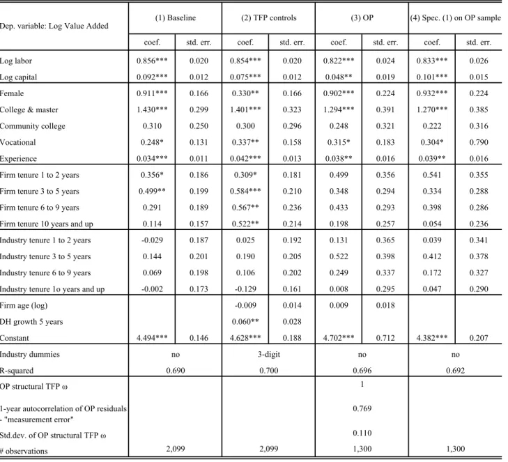
Log labor 0.856*** 0.020 0.854*** 0.020 0.822*** 0.024 0.833*** 0.026
Log capital 0.092*** 0.012 0.075*** 0.012 0.048** 0.019 0.101*** 0.015
Female 0.911*** 0.166 0.330** 0.166 0.902*** 0.224 0.932*** 0.224
College & master 1.430*** 0.299 1.401*** 0.323 1.294*** 0.391 1.270*** 0.385
Community college 0.310 0.250 0.300 0.296 0.248 0.321 0.222 0.316
Vocational 0.248* 0.131 0.337** 0.158 0.315* 0.183 0.304* 0.790
Experience 0.034*** 0.011 0.042*** 0.013 0.038** 0.016 0.039** 0.016
Firm tenure 1 to 2 years 0.356* 0.186 0.309* 0.181 0.499 0.356 0.541 0.355
Firm tenure 3 to 5 years 0.499** 0.199 0.584*** 0.210 0.348 0.294 0.334 0.288
Firm tenure 6 to 9 years 0.291 0.189 0.567** 0.236 0.433 0.293 0.398 0.286
Firm tenure 10 years and up 0.114 0.157 0.522** 0.214 0.198 0.257 0.054 0.236
Industry tenure 1 to 2 years -0.029 0.187 0.025 0.192 0.131 0.365 0.039 0.341
Industry tenure 3 to 5 years 0.144 0.201 0.190 0.205 0.522 0.398 0.412 0.378
Industry tenure 6 to 9 years 0.069 0.198 0.106 0.202 0.249 0.337 0.172 0.327
Industry tenure 1o years and up -0.002 0.173 -0.129 0.161 0.008 0.295 0.047 0.290
Firm age (log) -0.009 0.014 0.009 0.018
DH growth 5 years 0.060** 0.028 Constant 4.494*** 0.146 4.628*** 0.188 4.702*** 0.712 4.382*** 0.207 Industry dummies R-squared OP structural TFP ω Std.dev. of OP structural TFP ω # observations
(1) Nonlinear estimation of a labor quality augmented Cobb Douglas production function
(2) Adds log of firm age, firm growth over the last 5 years and 3 digit industry dummies as TFP controls
(3) OP 3rd stage: estimation of log value added on log labor quality, log capital, log firm age and OP structural TFP ω. See in the text for more information. OP 1st stage: the labor and labor quality coefficients were retrieved by re-estimating (1) with a second-order polynomial in capital, investment and firm age. OP 2nd stage: nonlinear estimation of log value added minus labor quality on capital, firm age and a polynomial in the estimate of unobserved productivity retreives the estimates of the coefficients on capital and firm age
(4) Similar to (1) but with the same sample as (3) ***/**/* reports significance at 1/5/10%
1,300 Table 3B - Labor Quality Augmented Production Function Estimates
Construction & Transportation
(4) Spec. (1) on OP sample
no 0.692
no 3-digit no
(1) Baseline Dep. variable: Log Value Added
2,099 1,300 (3) OP 0.690 0.700 0.696 (2) TFP controls 2,099 1 0.110 1-year autocorrelation of OP residuals
- "measurement error"
0.769
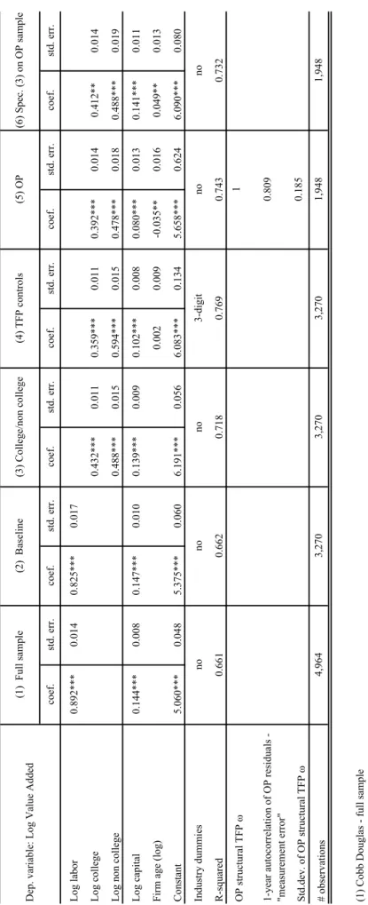
coef. std. err. coef. std. err. coef. std. err. coef. std. err. coef. std. err. coef. std. err. Log labor 0.892*** 0.014 0.825*** 0.017 Log college 0.432*** 0.011 0.359*** 0.011 0.392*** 0.014 0.412** 0.014
Log non college
0.488*** 0.015 0.594*** 0.015 0.478*** 0.018 0.488*** 0.019 Log capital 0.144*** 0.008 0.147*** 0.010 0.139*** 0.009 0.102*** 0.008 0.080*** 0.013 0.141*** 0.011
Firm age (log)
0.002 0.009 -0.035** 0.016 0.049** 0.013 Constant 5.060*** 0.048 5.375*** 0.060 6.191*** 0.056 6.083*** 0.134 5.658*** 0.624 6.090*** 0.080
Industry dummies R-squared OP structural TFP
ω
Std.dev. of OP structural TFP
ω
# observations (1) Cobb Douglas - full sample (2) Cobb Douglas - sample with no missing log college and log non college (3) Similar to (2) but with labor split into college vs. non college (4) Similar to (3), adds the log of firm age and 3 digit industry dummies as TFP controls. In a specification not shown, we add
firm growth over the last 5 years
as an extra control. The coefficients estimates and R-squared were very similar (5) OP 3rd stage: estimation of log value added on log college, log non college, log capital, log firm age and OP structural TF
P
ω
. See the text for more information.
OP 1st stage: the college and non college coefficients were retrieved by re-estimating (3) with a second-order polynomial in ca
pital, investment and firm age
OP 2nd stage: nonlinear estimation of (log value added - 0.268*log college - 0.468*log non college) on capital, firm age and a
polynomial in the estimate of unobserved
productivity retreives the estimates of the coefficients on capital and firm age (6) Similar to (3) but with the same sample as (5) ***/**/* reports significance at 1/5/10% no 0.661 0.662 0.718 no 4,964 3,270 3,270 3,270 (4) TFP controls 1 (5) OP 0.769
Table 4A - Production Function Estimates - Retail, Restaurants and Hotels
no
Dep. variable: Log Value Added
(1) Full sample (2) Baseline (3) College/non college (6) Spec. (3) on OP sample no no 3-digit 0.732 1,948 0.809 0.743 0.185 1,948
1-year autocorrelation of OP residuals - "measurement error"
coef. std. err. coef. std. err. coef. std. err. coef. std. err.
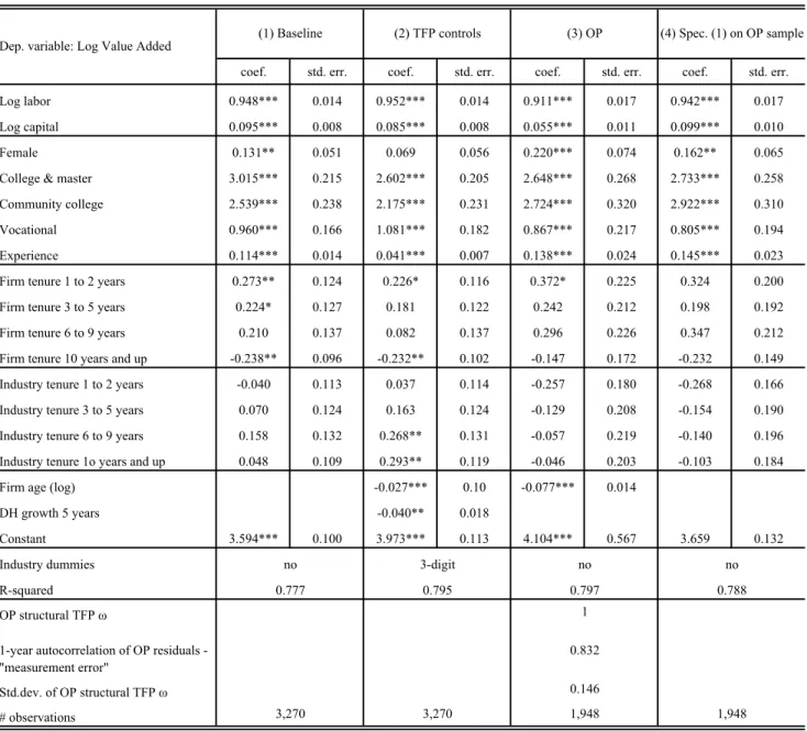
Log labor 0.948*** 0.014 0.952*** 0.014 0.911*** 0.017 0.942*** 0.017
Log capital 0.095*** 0.008 0.085*** 0.008 0.055*** 0.011 0.099*** 0.010
Female 0.131** 0.051 0.069 0.056 0.220*** 0.074 0.162** 0.065
College & master 3.015*** 0.215 2.602*** 0.205 2.648*** 0.268 2.733*** 0.258
Community college 2.539*** 0.238 2.175*** 0.231 2.724*** 0.320 2.922*** 0.310
Vocational 0.960*** 0.166 1.081*** 0.182 0.867*** 0.217 0.805*** 0.194
Experience 0.114*** 0.014 0.041*** 0.007 0.138*** 0.024 0.145*** 0.023
Firm tenure 1 to 2 years 0.273** 0.124 0.226* 0.116 0.372* 0.225 0.324 0.200
Firm tenure 3 to 5 years 0.224* 0.127 0.181 0.122 0.242 0.212 0.198 0.192
Firm tenure 6 to 9 years 0.210 0.137 0.082 0.137 0.296 0.226 0.347 0.212
Firm tenure 10 years and up -0.238** 0.096 -0.232** 0.102 -0.147 0.172 -0.232 0.149
Industry tenure 1 to 2 years -0.040 0.113 0.037 0.114 -0.257 0.180 -0.268 0.166
Industry tenure 3 to 5 years 0.070 0.124 0.163 0.124 -0.129 0.208 -0.154 0.190
Industry tenure 6 to 9 years 0.158 0.132 0.268** 0.131 -0.057 0.219 -0.140 0.196
Industry tenure 1o years and up 0.048 0.109 0.293** 0.119 -0.046 0.203 -0.103 0.184
Firm age (log) -0.027*** 0.10 -0.077*** 0.014
DH growth 5 years -0.040** 0.018 Constant 3.594*** 0.100 3.973*** 0.113 4.104*** 0.567 3.659 0.132 Industry dummies R-squared OP structural TFP ω Std.dev. of OP structural TFP ω # observations
(1) Nonlinear estimation of a labor quality augmented Cobb Douglas production function
(2) Adds log of firm age, firm growth over the last 5 years and 3 digit industry dummies as TFP controls
(3) OP 3rd stage: estimation of log value added on log labor quality, log capital, log firm age and OP structural TFP ω. See in the text for more information. OP 1st stage: the labor and labor quality coefficients were retrieved by re-estimating (1) with a second-order polynomial in capital, investment and firm age. OP 2nd stage: nonlinear estimation of log value added minus labor quality on capital, firm age and a polynomial in the estimate of unobserved productivity retreives the estimates of the coefficients on capital and firm age
(4) Similar to (1) but with the same sample as (3) ***/**/* reports significance at 1/5/10%
1,948 Table 4B - Labor Quality Augmented Production Function Estimates
Retail, Restaurants and Hotels
(4) Spec. (1) on OP sample no 0.788 3,270 3,270 1,948 (3) OP 1 0.777 0.795 0.797 0.146 no 3-digit no
Dep. variable: Log Value Added (1) Baseline (2) TFP controls
1-year autocorrelation of OP residuals - "measurement error"
0.832
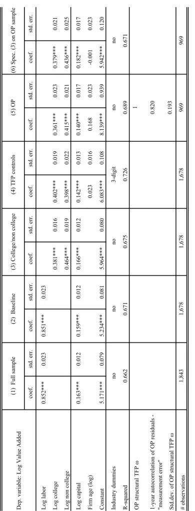
coef. std. err. coef. std. err. coef. std. err. coef. std. err. coef. std. err. coef. std. err. Log labor 0.852*** 0.023 0.851*** 0.023 Log college 0.381*** 0.016 0.402*** 0.019 0.361*** 0.023 0.379*** 0.021
Log non college
0.464*** 0.019 0.398*** 0.022 0.415*** 0.021 0.436*** 0.025 Log capital 0.163*** 0.012 0.159*** 0.012 0.166*** 0.012 0.142*** 0.013 0.140*** 0.017 0.182*** 0.017
Firm age (log)
0.023 0.016 0.168 0.023 -0.001 0.023 Constant 5.171*** 0.079 5.234*** 0.081 5.964*** 0.080 6.083*** 0.108 8.139*** 0.939 5.942*** 0.120
Industry dummies R-squared OP structural TFP
ω
Std.dev. of OP structural TFP
ω
# observations (1) Cobb Douglas - full sample (2) Cobb Douglas - sample with no missing log college and log non college (3) Similar to (2) but with labor split into college vs. non college (4) Similar to (3), adds the log of firm age and 3 digit industry dummies as TFP controls. In a specification not shown, we add
firm growth over the last 5 years
as an extra control. The coefficients estimates and R-squared were very similar (5) OP 3rd stage: estimation of log value added on log college, log non college, log capital, log firm age and OP structural TF
P
ω
. See the text for more information.
OP 1st stage: the college and non college coefficients were retrieved by re-estimating (3) with a second-order polynomial in ca
pital, investment and firm age
OP 2nd stage: nonlinear estimation of (log value added - 0.268*log college - 0.468*log non college) on capital, firm age and a
polynomial in the estimate of unobserved
productivity retreives the estimates of the coefficients on capital and firm age (6) Similar to (3) but with the same sample as (5) ***/**/* reports significance at 1/5/10%
no 0.662 0.671 0.675 no 1,843 1,678 1,678 1,678 (4) TFP controls 1 (5) OP 0.726
Table 5A - Production Function Estimates - Finance, Real Estate, R&D and Business Activities
no
Dep. variable: Log Value Added
(1) Full sample (2) Baseline (3) College/non college (6) Spec. (3) on OP sample no no 3-digit 0.671 969 0.820 0.689 0.193 969
1-year autocorrelation of OP residuals - "measurement error"