warwick.ac.uk/lib-publications
Manuscript version: Author’s Accepted Manuscript
The version presented in WRAP is the author’s accepted manuscript and may differ from the
published version or Version of Record.
Persistent WRAP URL:
http://wrap.warwick.ac.uk/132744
How to cite:
Please refer to published version for the most recent bibliographic citation information.
If a published version is known of, the repository item page linked to above, will contain
details on accessing it.
Copyright and reuse:
The Warwick Research Archive Portal (WRAP) makes this work by researchers of the
University of Warwick available open access under the following conditions.
Copyright © and all moral rights to the version of the paper presented here belong to the
individual author(s) and/or other copyright owners. To the extent reasonable and
practicable the material made available in WRAP has been checked for eligibility before
being made available.
Copies of full items can be used for personal research or study, educational, or not-for-profit
purposes without prior permission or charge. Provided that the authors, title and full
bibliographic details are credited, a hyperlink and/or URL is given for the original metadata
page and the content is not changed in any way.
Publisher’s statement:
Please refer to the repository item page, publisher’s statement section, for further
information.
SVS-JOIN:
Efficient
Spatial
Visual
Similarity
Join
for
Geo-Multimedia
LEI ZHU 1, WEIREN YU2,3, CHENGYUAN ZHANG 1, ZUPING ZHANG 1, FANG HUANG1, AND HAO YU1
1SchoolofComputerScienceandEngineering,CentralSouthUniversity,Changsha410083,China
2SchoolofComputerScienceandTechnology,NanjingUniversityofScienceandTechnology,Nanjing210094,China
3DepartmentofComputerScience,UniversityofWarwick,CoventryCV47AL,U.K. Correspondingauthor:ChengyuanZhang([email protected])
ThisworkwassupportedinpartbytheNationalNaturalScienceFoundationofChinaunderGrant61702560,Grant61379109,Grant 61836016,andGrant61972203,inpartbytheScienceandTechnologyPlanofHunanProvinceunderProject2018JJ3691andProject 2016JC2011,inpartbytheNaturalScienceFoundationofJiangsuProvinceunderGrantBK20190442,andinpartbytheResearchand InnovationProjectofCentralSouthUniversityGraduateStudentsunderGrant2018zzts177.
ABSTRACT In the big data era, massive amount of multimedia data with geo-tags has been generated and collected by smart devices equipped with mobile communications module and position sensor module. This trend has put forward higher request on large-scale geo-multimedia retrieval. Spatial similarity join is one of the significant problems in the area of spatial database. Previous works focused on spatial textual document search problem, rather than geo-multimedia retrieval. In this paper, we investigate a novel geo-multimedia retrieval paradigm named spatial visual similarity join (SVS-JOIN for short), which aims to search similar geo-image pairs in both aspects of geo-location and visual content. Firstly, the definition of SVS-JOIN is proposed and then we present the geographical similarity and visual similarity measurement. Inspired by the approach for textual similarity join, we develop an algorithm named SVS-JOINBby combining the PPJOIN
algorithm and visual similarity. Besides, an extension of it named SVS-JOINGis developed, which utilizes
spatial grid strategy to improve the search efficiency. To further speed up the search, a novel approach called SVS-JOINQ is carefully designed, in which a quadtree and a global inverted index are employed.
Comprehensive experiments are conducted on two geo-image datasets and the results demonstrate that our solution can address the SVS-JOIN problem effectively and efficiently.
INDEX TERMS Geo-image, geographical similarity, similarity join, visual similarity.
I. INTRODUCTION
In the big data era, online social networking services, search engine and multimedia sharing services are rapidly growing in popularity, which generate, collect and store large-scale multimedia data [1]–[4], e.g., texts, images, audios and videos. For example, we use online social networking ser-vices such as Facebook,1 Twitter,2 Linkedin,3 Weibo,4 etc. to make friends, sharing hobbies and work information by posting texts, uploading images or short videos. On the other hand, for multimedia data [5] sharing platforms such as
Flickr,5 more than 3.5 million new images posted online every day in March 2013. Every minute there are 100 hours of videos uploaded to YouTube,6and more than 2 billion videos totally stored in this platform by the end of 2013. In China, IQIYI7is the largest video sharing web site. The total watch time monthly of this online video service exceeded 42 billion minutes. These multimedia online services not only provide great convenience for us, but create possibilities for the gener-ation, collection, storage and sharing of large-scale multime-dia data [6], [7]. Moreover, this trend has put forward greater challenges for massive multimedia data retrieval [8], [9].
Smartphones and tablets equipped with communications module (e.g., WiFi and 4G module) and position sensor mod-ule (e.g., GPS-Modmod-ule) collect huge amounts of multimedia
5https://www.flickr.com/ 6https://www.youtube.com/ 7http://www.iqiyi.com/ 1https://facebook.com/ 2http://www.twitter.com/ 3https://www.linkedin.com/ 4https://weibo.com/
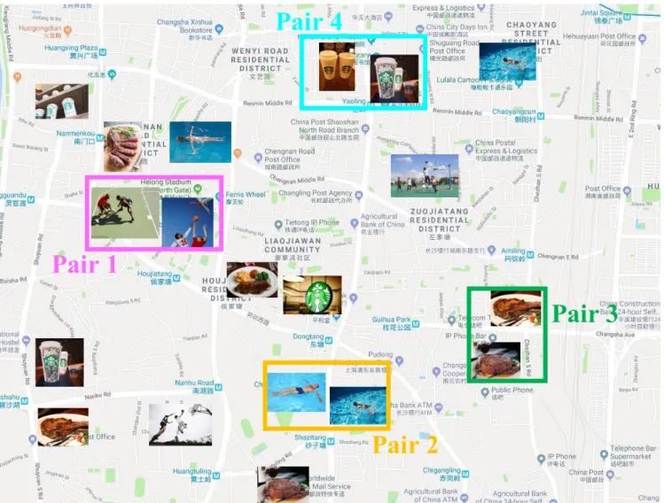
FIGURE 1. An example of spatial visual similarity join.
data [10]–[12] with geo-tags. For example, users can take photos or videos [13], [14] with the geo-location informa-tion. Besides, many mobile applications such as WeChat, Twitter and Instagram support posting, storing and sharing geo-multimedia data. Other location-based services such as Google Places, Yahoo!Local, and Dianping provide the con-venient query services by taking into account both geograph-ical proximity and multimedia content similarity.
Motivation:Due to the wide application of smart devices and location-based services, spatial textual search problem has become a hot spot in the area of spatial database and information retrieval. Lots of spatial indexing techniques have been proposed to support efficient query, such as R-Tree [15], R+-Tree [16], R∗-Tree [17], KR∗-Tree [18], IR2-Tree [19] etc. More recently, Denget al. [20] studied a generic version of closest keywords search called best keyword Cover. Cao et al. [21] proposed the problem of collective spatial keyword querying, Fan et al.[22] studied the problem of spatio-textual similarity search for regions
of interests query. Zhanget al. [23] proposed IL-Quadtree to address top-kspatial keyword search problem efficiently. However, these researches just only consider the textual data such as keywords, they do not take into account the con-tent of multimedia data, e.g. images. One of the significant geo-textual search problems, spatial textual similarity join, is to find out the spatial textual object pairs that are similar in both aspects of geo-location and textual content simultane-ously. It has attracted wide attention such as [24]–[29]. Nev-ertheless, there is no work pays attention to geo-multimedia data for this task. In this paper, we aim to investigate a novel paradigm named Spatial Visual Similarity JOIN
(SVS-JOIN) and develop an efficient solution to overcome the challenge of geo-multimedia query. Fig.1is a simple but intuitive example to describe this problem.
Example 1: As illustrated in Fig. 1, the spatial visual similarity join can be applied in friends recommendation services on online social networking services. According to the geo-images posted by the users, the social networking
system can find the similar geo-images in both aspects of geo-location and visual content. It is easy to understand that two people may make friend if they have the same hob-bies and their position is very close. There are four similar geo-image pairs in Fig.1are searched out. For pair 1 shown in magenta rectangle, two users who took the photos about basketball at two close places are very likely to become good friends.
To the best of our knowledge, this paper is the first time to study the SVS-JOIN problem. We introduce the definition of spatial visual similarity join in formal and present the relevant notions. Besides, we discuss how to measure geographical similarity and visual similarity to find the similar geo-image pairs. To measure visual similarity accurately, we employ two types of visual features to generation visual representa-tions of geo-images: (1) the traditional hand-crafted visual features named Scale-Invariant Features Transform (SIFT for short) and (2) deep visual features extracted by con-volutional neural networks (CNN for short). The former is named SIFT-BoVW and the latter is called Deep-BoVW. To combat this challenge effectively and efficiently, an algo-rithm called SVS-JOINB inspired by the techniques used in
textual similarity join is introduced. Based on it, we develop an extension of SVS-JOINB called SVS-JOING which uses
spatial grid partition strategy to improve the efficiency. In order to further improve the search performance, a novel method named SVS-JOINQ is carefully designed, which is
based on quadtree and global inverted index to speed up search.
Contributions:Our main contributions can be summarized as follows:
• To the best of our knowledge, this work is the first
to study the problem of spatial visual similarity join. We propose the definition of geo-image, SVS-JOIN and relevant notions. The visual similarity function and geographical similarity function are designed for similar geo-image pair search.
• For the visual representation of geo-images, we propose to employ CNN to extract deep visual features for visual words generation, rather than hand-crafted visual fea-tures. We call this method Deep-BoVW that is a com-bination of deep CNN techniques, Bag-of-Visual-Words andk-means clustering method. As far as we know, there is no existing research that uses the combination of CNN and BoVW to address the image JOIN problem.
• We introduce an algorithm named SVS-JOINBinspired
by the techniques used for the problem of textual sim-ilarity join. An extension of SVS-JOINB called
SVS-JOING is developed which utilizes spatial grid
parti-tion technique to speed up search. To further improve the searching performance, we present a novel method named SVS-JOINQ that is based on quadtree partition
technique and a global inverted index.
• We have conducted comprehensive experiments on real geo-image dataset. Experimental results demonstrate that our approach has really high performance.
Roadmap:The remainder of this paper is organized as fol-lows: In SectionIIwe introduce the previous researches con-cerning content-based image retrieval, spatial textual search and set similarity joins, which are related to this work. In SectionIII, we propose the definition of spatial visual sim-ilarity join and relevant concepts. In SectionIV, two visual representations named SIFT-BoVW and Deep-BoVW are presented. Besides, we introduce a baseline and an extension named SVS-JOINB and SVS-JOING respectively. In
addi-tion, a novel algorithm named SVS-JOINQ is proposed,
in which a combination of a quadtree and a global inverted indexing structure is employed to solve the SVS-JOIN prob-lem more efficiently. In SectionV, we present the experiment results. Finally, we conclude the paper in SectionVI.
II. RELATED WORK
In this section, we introduce the previous studies of content-based image retrieval, spatial textual search and set similarity joins, which are relevant to this work. To the best of our knowledge, no priori work on this problem.
A. CONTENT-BASED IMAGE RETRIEVAL
1) CBIR VIA SIFT
As one of the most important problems, content-based image retrieval (CBIR for short) [30]–[32] has gained much atten-tion of many researchers in multimedia area [33]–[35]. Scale-Invariant Features Transform (SIFT for short) [36], [37] is one of the conventional methods for visual fea-ture extraction. It transforms an image into a collection of local feature vectors. These features are invariant to transla-tion, scaling, rotatransla-tion, and partially invariant to illumination changes. In recent years, lots of works have been proposed using SIFT to overcome CBIR challenges. For example, Mortensenet al. [39] proposed a feature descriptor which augments SIFT with a global context vector that adds curvi-linear shape information from a much larger neighborhood. Keet al.[40] proposed a SIFT and PCA based method to encode the salient aspects of the image gradient in the neigh-borhood of feature point. Suet al.[41] presented horizontal or vertical mirror reflection invariant binary descriptor named MBR-SIFT to solve the problem of image matching. To gain sufficient distinctiveness and robustness for the task of feature matching, Li and Ma [42] designed a novel SIFT based fea-ture descriptor by integrating color and global information. Zhu et al. [43] proposed an image registration algorithm called BP-SIFT by using belief propagation, which has sig-nificant improvement for the problem of keypoint matching.
2) CBIR VIA BoVW
Originated from text retrieval and mining, BoVW is an impor-tant visual representation method in multimedia retrieval and computer vision [5], [11], [44], [45]. BoVW [46] is a con-ventional image representation model, which is to improve the performance of image feature matching markedly. For image retrieval problem, it generates visual words by utilizing
presented an evolutionary algorithm to implement an auto-matically learning weighting schemes of this model for computer vision tasks. Dimitrovski et al. [48] proposed to use predictive clustering trees (PCTs) to improve the BoVW image retrieval in the large-scale image database. Mandal et al. [49] proposed a patch-based framework by using SIFT descriptor and BoVW model to improve the performance of handwritten signature detection. Based on S-BoVW paradigm, dos Santoset al.[50] proposed a novel method that considers information of texture to generate tex-tual signatures of image blocks. For the task of Medical image retrieval, Zhanget al.[51] proposed a BoVW based medical image retrieval approach named PD-LST retrieval to iden-tify discriminative characteristics between different medical images with pruned dictionary. Karakasiset al.[52] proposed a BoVW based framework for image retrieval, which uses affine image moment invariants as descriptors of local image areas.
3) CBIR VIA DEEP LEARNING
As a powerful tool, deep learning [53]–[55] is widely used to solve image retrieval [56]–[58] and computer vision prob-lems. In 2012, AlexNet [59] proposed by Krizhevskyet al.
significantly improves the accuracy of image retrieval. More recently, lots of deep learning based researches have been proposed for CBIR task. Gordoet al.[60] proposed to gen-erate compact global signatures via CNN for image retrieval. Fuet al. [61] utilized CNN to generate visual features and employed SVM for classification. Tzelepi et al. [62] pro-posed a novel CNN based approach that exploits the data label information to generate better descriptors for image retrieval. For style based image retrieval task, Matsuo and Yanai [63] proposed to use style vector that is transformed from CNN based style matrix. Zhou et al.[64] proposed a CNN-based match kernel to encode CNN feature and SIFT feature to improve the accuracy. Liu et al. [65] combined high-level CNN features and low-level DDBTC features to generate two-layer codebook features for performance boost-ing. Seddatiet al.[66] proposed to improve Regional Max-imal Activation (RMAC) approach by combined multi-scale and multi-layer feature extraction of different RMAC exten-sions. Yanget al.[67] utilized a dynamic match kernel with deep CNN features to search images with different content details but similar semantics. Shimoda and Yanai [68] tested simple, siamese and triplet CNN to generate good visual fea-tures for food image retrieval. For some specific application, Nakazawa and Kulkarni [69] presented a CNN based image classification method to solve wafer maps defect pattern recognition issue. Sarraf and Tofighi [70] employed CNN to recognize fMRI image of Alzheimer’s brain from normal healthy brain.
It is no doubt that these solutions improve the perfor-mance of image retrieval and visual feature matching sig-nificantly. However, these works cannot solve the problem of geo-multimedia data retrieval as they have no effective processing for geographical distance measurement.
B. SPATIAL TEXTUAL SEARCH
1) SPATIAL TEXTUAL QUERY
Due to the collection and storage of large scale spatial tual data, there has been increasing interest on spatial tex-tual search problem [71], [72]. Spatial textex-tual search [23], [73], [74] aims to retrieve textual objects or documents with geo-tags by textual similarity and geographical proximity. For top-kspatial keyword queries, Rocha-Junioret al.[75] pro-posed a novel spatial index named Spatial Inverted Index (S2I for short) to enhance the efficiency of search. Liet al.[76] proposed an efficient indexing structure named IR-tree, which enables spatial pruning and textual filtering to be performed simultaneously. Zhang et al. [77] presented a scalable integrated inverted index called I3 that uses the Quadtree to hierarchically partition the data space into cells. Zhanget al.[78] proposed an efficient index named inverted linear quadtree (IL-Quadtree for short) and designed a novel algorithm to improve the performance of query. Liet al.[79] presented BR-tree to solve the problem of keyword-based
k-nearest neighbor queries. They utilized R-tree to maintain the spatial information of objects and exploited B-tree to main the terms in the objects. Fanet al.[22] proposed grid-based signatures and threshold-aware pruning techniques to address spatio-textual similarity search problem. Zhanget al. [80] proposed to model the spatial keyword search problem as a top-kaggregation problem. They developed a rank-aware CA algorithm that works well on inverted lists sorted by textual relevance and spatial curving order. Wanget al.[81] proposed an efficient technique named AP-Tree to solve the problem of continuous spatial-keyword queries over streaming data. Zhanget al.[82] introducedm-closest keywords (mCK for short) query that aims to search out the spatially closest tuples which match m user-specified keywords. Guo et al. [83] proposed another solution to solve themCK search problem. They devised a novel greedy algorithm namedSKECthat has an approximation ratio of 2 and in addition, they developed two approximation algorithms calledSKECaandSKECa+
respectively to improve the efficiency.
2) SET SIMILARITY JOINS
In recent years, lots of researchers paid attentions on the problem of spatial textual similarity join [24], [84], [85]. A spatial similarity join of two spatial databases aims to search out pairs of objects that are simultaneously similar in both aspects of textual and spatial. Ballesteroset al.[25] proposed an algorithm based on MapReduce parallel pro-gramming model to solve this problem on large-scale spatial databases. Efstathiades et al. [26] propose the problem of Spatio-Textual Point-Set Join query and extended the exist-ing methods to solve the spatial-textual joins problem of point sets. Huet al. [27] introduced a signature-based join framework that prunes large numbers of dissimilar pairs to enhance the search efficiency. To overcome the issue of large number of duplicates, Rong et al. [28] introduced a novel duplicate free framework with three filtering methods to
TABLE 1. The summary of notations.
prune dissimilar string pairs without computing their similar-ity scores. Shanget al.[29] presented a knowledge hierarchy based filter-and-verification framework to efficiently identify the similar pairs to address knowledge-aware similarity join problem.
These spatial textual search and similarity joins approaches only consider the textual and spatial information, that means they cannot be directly applied to address geo-image joins problem even if they raise search efficiency substantially. Thus, this paper proposes to combine geographical informa-tion and visual representainforma-tions of geo-images to construct efficient search algorithms for spatial visual similarity joins problem.
III. PRELIMINARIES
In this section, we propose the definition of spatial visual similarity joins (SVS-JOIN) at the first time, then present the geographical and visual similarity measurement. Besides, we briefly introduce the SIFT and CNN techniques respec-tively, which are the base of our work. Table1summarizes the notations frequently used throughout this paper to facilitate the discussion.
A. PROBLEM DEFINITION
Definition 1 (Geo-Image): LetDI = {I1,I2, . . . ,I|DI|}be
a geo-image dataset,|DI|denotes the size ofDI. A geo-image
Ii ∈DI is defined as a tupleIi =<Ii.G,Ii.V >, whereIi.G
is the geographical information component that is generated from the geo-tag of this image. More specifically, it consists of longitudeX and latitudeY, i.e.,Ii.G = (X,Y). Another
part,Ii.V, is the visual information component that consists of
a visual word setIi.V = {v1,v2, . . . ,vn}modeled by BoVW.
iis the id of the geo-image.
Consider two geo-image datasetsRI = {I1r,I2r, . . . ,I|rRI| }
andSI = {I1s,I2s, . . . ,I|sSI|}, similar to spatial textual
sim-ilarity join, a spatial visual simsim-ilarity join aims to retrieval all pairs of geo-images fromRI andSI respectively, which
are similar enough in both aspects of geo-location and visual content. We introduce two thresholds, i.e., geographical sim-ilarity threshold and visual simsim-ilarity threshold to measure these two similarity. Specifically, for each pair, both of the geographical similarity and visual similarity of these two geo-images are less than geographical similarity threshold and visual similarity threshold. To clarify our work more clearly, we propose the definition of spatial visual similarity join as follows.
Definition 2 (Spatial Visual Similarity Join (SVS-JOIN)):
Given two geo-image datasetsRI = {I1r,I2r, . . . ,I|rR
I|}and SI = {I1s,I2s, . . . ,I|sSI|}, geographical similarity threshold0G
and visual similarity threshold0V. A spatial visual similarity
join denoted as SVS-JOIN(R,S, 0G, 0V) returns a set of
geo-image pairsP ⊆ R×S, in which each pair contains two highly similar geo-images in both aspect of geo-location and visual content, i.e.,
P = {(Iir,Ijs)|GeoSim(Iir,Ijs)≤0G, VisSim(Iir,Ijs)≥0V,
∀Iir ∈RI,Ijs ∈SI} (1)
whereGeoSim(Iir,Ijs) andVisSim(Iir,Ijs) are the geographical similarity function and visual similarity function respectively. To measure these two similarities quantitatively, we uti-lize Euclidean distance measurement and Jaccard distance measurement to implement these two functions, shown as follows.
Definition 3 (Geographical Similarity Function): Given two geo-image datasetsRI = {I1r,I2r, . . . ,I|rRI|}andSI = {I1s,I2s, . . . ,I|sS
I|}, ∀I
r
i ∈ RI,Ijs ∈ S, the geographical
similarity betweenIir andIjs is measured by the following similarity function:
GeoSim(Iir,Ijs)= EucDis
(Iir,Ijs)
MaxDis(R,S) (2)
whereEucDst(Iir,Ijs) is the Euclidean distance between Iir
andIjs, which is measured by the following function: EucDis(Iir,Ijs)=
q
(Iir.G.X−Ijs.G.X)2+(Ir
i.G.Y−Ijs.G.Y)2
FIGURE 2. An example of geo-images and spatial visual similarity join.
the function MaxDis(R,S) is to return the maximum Euclidean distance between any two geo-images fromRand
Srespectively, which is described in formal as follows: MaxDis(R,S)=max({EucDis(Iir,Ijs)|Iir∈R,Ijs∈S}) (4) where the functionmax(·) is to return the maximum element from a set.
Definition 4 (Visual Similarity Function): Given two geo-image datasets RI = {I1r,I2r, . . . ,I|rRI|} and SI = {I1s,I2s, . . . ,I|sS
I|},∀I
r
i ∈ RI,Ijs ∈ S, the visual similarity
between Iir andIjs is measured by the following similarity function: VisSim(Iir,Ijs)= P v∈Iir.V∩Ijs.Vw(v) P v∈Iir.V∪Ijs.Vw(v) (5) where w(v) represents the weight of the visual word v. In this work, we measure the weight of visual word by term frequency-inverse document frequencytf-idf [86].
Assumption:For ease of discussion, here we assume that
R=S. Our approach can be applied well in the case ofR6= S. Therefore, for a geo-image datasetR, we denote a spatial visual similarity join as SVS-JOIN(R, 0G, 0V).
Example 2: We give a simple example to describe how to perform a SVS-JOIN search. Consider a geo-image dataset
R= {I1,I2, . . . ,I9}, shown in Fig.2. The upper left figure is
the geographical distribution of the geo-images in R. The upper right figure shows this geo-image dateset, in which each geo-image is represented by a set of visual words.
At the right bottom is the list of these visual words, and their weights are shown at the left bottom. We set 0G = 0.3
and0V = 0.4, the SVS-JOIN(R,0.3,0.4) returns the set
P= {(I3,I6),(I4,I9)}.
B. SCALE-INVARIANT FEATURES TRANSFORM
Our first visual representation scheme uses SIFT [36], [37]. This conventional technique aims to transform an image into a large set of local feature vectors, which are invariant to image translation, scaling, and rotation, and partially invari-ant to illumination changes and affine or 3D projection. It has four main phases:
1) SCALE-SPACE EXTREMA DETECTION
The first phase is called scale-space extrema detection. This method searches all the images in scale space, which is to identify potential points of interest that are invariant to scale and orientation by utilizing difference-of-Gaussian (DoG) function.
2) KEYPOINT LOCALIZATION
The second phrase is named keypoint localization, which is to select and localize the keypoints according to their stability. At each candidate location, a fine fitting model is used to determine the location and scale.
3) ORIENTATION ASSIGNMENT
In the orientation assignment phrase, according to the local gradient direction of the image, each keypoint is assigned one or more directions, and all subsequent operations transform
FIGURE 3. An example of convolutional neural network. A typical CNN model has three main parts: Input layer, convolutional and pooling layer, and full-connected layer.
the direction, scale and position of the keypoints to provide invariance of features to these transformations.
4) KEYPOINT DESCRIPTOR
In the last phase, the local gradients of the image are mea-sured around each feature point at selected scales. And these gradients are transformed into a representation which allows for significant local shape distortion and illumination trans-formation.
C. CONVOLUTIONAL NEURAL NETWORKS
Convolutional Neural Network (CNN for short) was first proposed by Yann Lecun in 1998 [38]. A typical CNN shown in Fig. 3 consists of several convolutional layers, pooling layers and fully-connected layers. The convolutional layer and pooling layer cooperate to form multiple convolution groups, extract visual features from low-level to high-level layer by layer, and finally complete classification through several full-connected layers. CNN simulates feature differ-entiation by convolutional operation, and reduces the number of model parameters by weight-sharing and pooling. The superiority of the CNN originates from four key ideas [53]: (1) local connections, (2) shared weights, (3) pooling and (4) the use of many layers.
This powerful technique has been applied successfully in many tasks, e.g., image retrieval, visual understanding, pattern classification, etc. In this work, we employ CNN as the second method of visual representation.
IV. METHODOLOGY
In this section, we introduce a novel framework to solve the problem of SVS-JOIN. This framework support two schemes for visual words generation: the one utilizes hand-crafted visual features, namely SIFT in a conventional manner; the other is to produce visual words by generating deep visual representations via CNN, which is a better method to cap-ture high-level semantic concepts from inputs. In addition, inspired by the algorithm of textual similarity joins, we intro-duce a baseline named SVS-JOINB and propose a spatial
grid partition based algorithm for SVS-JOIN task called
SVS-JOING. As an alternative approach of SVS-JOING,
a novel quadtree based global index method named
SVS-JOINQ is designed, which can speed up the search
significantly.
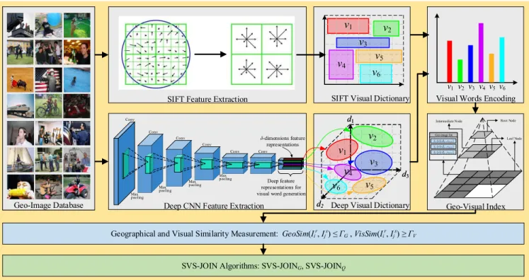
A. OVERVIEW OF THE FRAMEWORK
Fig. 4 illustrates the proposed framework for SVS-JOIN problem. As discussed above, SVS-JOIN is a geo-image-oriented search problem that means the input of the sys-tem is a geo-image database. Therefore, the first priority is to generate the representations of geo-images. Two visual representation schemes are proposed in this framework: the one utilizes hand-crafted visual features that are generated via SIFT descriptor in a conventional manner, and then use BoVW model to produce visual words for each geo-image, this scheme is called SIFT-BoVW. The other scheme is to produce visual words by generating deep visual repre-sentations via a CNN model, which is a better method to capture high-level semantic concepts from inputs. Similar to the first scheme, we build the deep visual dictionary based on these feature representations generated by CNN and rep-resent all the geo-images by deep visual words. We call this schemeDeep-BoVW. Clearly, these two visual representa-tion schemes are all based on BoVW model, which is the basis of our geo-image index technique. In this work, two geo-image index structures are carefully designed: The first is a combination of spatial grid partition and inverted index, and the second one is a quadtree partition based inverted index. Based on these two index and similarity measurement
GeoSim(Iir,Ijs) andVisSim(Iir,Ijs), we develop two efficient SVS-JOIN algorithms, namely SVS-JOINGand SVS-JOINQ.
B. VISUAL REPRESENTATION SCHEMES
In this subsection, we introduce the two visual representation schemes in details, namely SIFT-BoVW and Deep-BoVW. Both of them are based on BoVW model. To represent a geo-image as a collection of visual words, we propose to use two different method to generate the visual word representa-tion, namely SIFT and Deep CNN.
1) SIFT-BoVW
In this scheme, Dense-SIFT technique, an extension of SIFT is employed to extract visual features from geo-images. In other words, it maps each geo-image into a 128-dimensions feature vector. After that we utilize k-means clustering method to construct SIFT visual dictionary by converting feature vectors into visual words. Let {I1,I2, . . . ,In}be a
set of geo-images, the feature vectors of them are denoted by{ξ1,ξ2, . . . ,ξ
n} = SIFT({I1,I2, . . . ,In}), whereSIFT(·)
is the SIFT feature extractor. According to the distance between these SIFT feature vectors,k-means method groups these feature vectors into k clusters G = {g1,g2, . . . ,gk}
which can be formulated by the following objective function:
Fk−means= arg min
G={gi}ki=1 k X i=1 gi X ξj∈gi kξj−χik2 2 (6)
where χi is the mean vector of the cluster gi, namely,
χi = |g1i| P
ξ∈giξ. L2 norm is used to measure the
FIGURE 4. The framework to solve the SVS-JOIN problem. Best view in color. This framework supports two schemes for visual words generation: the one utilizes hand-crafted visual features, namely SIFT in a conventional manner; the other is to produce visual words by generating deep visual
representations via CNN, which is a better method to capture high-level semantic concepts from inputs. Besides, based on the visual word
representations and geographical information, two geo-visual index structures are integrated in this framework to organize geo-images efficiently: The first method is a combination of spatial grid partition and inverted index, and the second one is a quadtree partition based inverted index. Based on these two index techniques and geographical and visual similarity measurementGeoSim(Iir,Ijs) andVisSim(Iir,Ijs), two efficient SVS-JOIN algorithms are developed, namely SVS-JOINGand SVS-JOINQ.
vector. After the clustering, the SIFT visual dictio-nary with k visual words has been constructed, namely
{v1,v2, . . .vk} = KMEANS({ξ1,ξ2, . . . ,ξn}), where
KMEANS(·) is the k-means algorithm. The SIFT visual dictionary is used to encode each geo-image by a k -dimensions vector that is the statistics of each visual word. As mentioned in Definition 4, we measure the weight of visual word by tf-idf, namely, {w(v1),w(v2), . . .w(vk)} =
TF-IDF({η(v1), η(v2), . . . η(vk)}), where η(·) denotes the
number of occurrences of a visual word in an image.
2) Deep-BoVW
As the second and more powerful scheme, we propose to integrate deep CNN and BoVW model to generate the deep visual word representation named Deep-BoVW. Compared with SIFT based method, the feature extraction in a deep convolutional manner can capture the rich high-level seman-tic concepts, which is more powerful than conventional hand-crafted features with little semantic information. The process is quite similar to SIFT-BoVW: a deep CNN extract visual features from low-level to high-level layer-by-layer, and then a deep visual dictionary is built on these visual features by k-means algorithm, which are used to encode geo-images.
Specifically, we employ a pre-trained deep CNN model, namely AlexNet [59], for the task of visual feature extraction. AlexNet consists of five convolutional layers, some of which
are followed by max-pooling layers, three fully-connected layers and a 1000-way softmax layer that is used to classifi-cation. In this work, the input images are resized as 227×227 pixels, and we use the fifth convolutional feature representa-tions with the size 13×13×256 to generate deep visual dictionary. For geo-image set{I1,I2, . . . ,In}, the deep visual
representation set of them is denoted by{ζ1,ζ2, . . . ,ζn} = CONV({I1,I2, . . . ,In};θ), wherein CONV(·;θ) is the deep
convolutional feature extractor,θis the network parameters, and∀ζi ∈ {ζ1,ζ2, . . . ,ζn},ζi = (ζi(1), ζi(2), . . . , ζi(256))T is a deep visual feature representation of an image. There-fore, Like SIFT-BoVW, the deep visual dictionary can be generated by k-means algorithm, namely {v1,v2, . . .vk} =
KMEANS({ζ1,ζ2, . . . ,ζn}). Likewise, the visual word encoding process is denoted by{w(v1),w(v2), . . .w(vk)} =
TF-IDF({η(v1), η(v2), . . . η(vk)}).
No doubt, AlexNet is definitely not the only choice for feature extraction. And actually in the experiments we also employ two other off-the-shelf CNN models, i.e., VGGNet-16 [87] and GoogLeNet [88] to take this job for performance evaluation. VGGNet is a powerful deep convolution neural network developed by Oxford University Computer Vision group and DeepMind researchers in 2014, and GoogLeNet is another outstanding deep CNN model during that year, which utilizes a novel structure named Inception. Both of them are very powerful for computer vision tasks. To facil-itate the discussion, we name these CNN based schemes as
AlexNet-BoVW, VGGNet-BoVW and GoogLeNet-BoVW respectively during the comparative experiments.
C. THE BASELINE FOR SPATIAL VISUAL SIMILARITY JOINS
In this section, we propose the baseline for the SVS-JOIN problem. Firstly, we introduce the state-of-the-art algorithm named PPJOIN [90] for textual similarity joins, which is utilized in our baseline. Then we present our baseline named SVS-JOINBin detail.
1) THE METHOD FOR TEXTUAL SIMILARITY JOINS
a: INVERTED INDEX BASED METHOD
The traditional way to solve textual similarity joins efficiently is to build an inverted index for the target object datasetR, which associates each word in the global word setW built beforehand to an objects inverted list L. For each object
o ∈ R, the inverted list L(v) of each word w ∈ o.V is traversed, whereo.V represents the keywords set ofo. Then we account the number of word overlap ofowith every object
ˆ
o ∈ L(v) and save these numbers in a seto. To facilitate
exploration of this method, we denoteo[oˆ] as the number
of word overlap ofo withoˆ. Apparently, the candidate pair set can be generated from o directly. Then for all objects
ˆ
o ∈ o, ifo[oˆ] > 0 andTxtSim(o,oˆ) ≥ θt, then the pair
(o,oˆ) can be one of the results. To describe this process in a formal way, textual similarity joins by this method is to return a result setP,
P= {(o,oˆ)|o∈R,oˆ∈o, o[oˆ]>0and TxtSim(o,oˆ)≥θt}
(7) whereTxtSim(o,oˆ) is the textual similarity function andθtis
the textual similarity threshold.
b: PREFIX FILTERING PRINCIPLE
When we use the inverted index based method, the inverted list Lwwill be quite long if the wordwis very frequent in
the dataset. This become a major challenge since a lot of can-didate pairs have to be generated in this situation. To reduce the size of the candidate set, an efficient method called prefix filtering principle was devised by [89]. According to this technique, we generate a global word ordering8that sorts keywords by word frequency in reverse order, and then for all objectso ∈ R, order the keywords ino.V by8. After the ordering, the prefix ofo.V is denoted asPf(o.V) and the length of it is denoted as|Pf(o.V)|, which is measured by the following equation:
|Pf(o.V)| = |o.V| − dθt|o.V|e +1 (8) where|o.V|represents the number of keywords ino.V,θt is
the textual similarity threshold. It is obvious that the length of prefix of an object is determined by the number of keywords contained by this object and the similarity threshold given in advance. According to this principle, we can get the following theorem:
Algorithm 1PPJOIN Algorithm
1: INPUT:Ris an objects dataset sorted by a global order-ing8,θtis a textual similarity threshold.
2: OUTPUT:P is the result pairs set.
3: foreachw∈Wdo 4: Lw← ∅; 5: end for 6: foreacho∈Rdo 7: |Pf(o.V)|S← |o.V| − dθt|o.V|e +1; 8: |Pf(o.V)|I ← |o.V| − d 2θt θt+1|o.V|e +1; 9: fori=1 to|Pf(o.V)|Sdo 10: w←thei-th keyword ino.V; 11: fore(oˆ,ioˆ)∈Lwand| ˆo.V| ≥θt|o.V|do 12: ifQualifyPosFilter(o,io,oˆ,ioˆ) && QualifySufFilter(o,io,oˆ,ioˆ)then 13: o[oˆ]←o[oˆ]+1; 14: else 15: o[oˆ]← −∞; 16: end if 17: end for 18: ifio≤ |Pf(o.V)|Ithen 19: Lw←Lw∪ {(o,io)}; 20: end if 21: end for 22: Verify(o, o,P); 23: end for 24: return P;
Theorem 1: Given two objects o,oˆ ∈ R and a textual similarity thresholdθt, if TxtSim(o,oˆ)≥θt, thenPf(o.V)∩
Pf(oˆ.V)6= ∅.
Obviously, the basic idea of Theorem1is that if the textual similarity between two objects is larger than a threshold, they should share same keywords. Therefore, this theorem can be used to prune the candidate pair set effectively. Specifically, for each objecto, we just only to search the keywords con-tained in the prefix ofo.
c: THE PPJOIN ALGORITHM
PPJOIN is one of the efficient algorithms to solve the textual similarity joins problem, developed by Xiaoet al.[90]. This algorithm is a combination of positional filtering and prefix filtering-based algorithm.
Algorithm1demonstrates the pseudo-code of the PPJOIN algorithm. The input of this algorithm is a textual similarity thresholdθtand an objects datasetRthat is sorted in
ascend-ing order of their size. At first, in Lines 3 to 5, it generates inverted listLwfor each word in the global words set. Then
from Line 6 to line 23, this algorithm traverses every objects in the input datasetRand find the similar pairs of objects. Specifically, for each object o ∈ R, probe prefix length
|Pf(o.V)|Sand|Pf(o.V)|Iare (Lines 7-8). Then from the first position to the|Pf(o.V)|S-th position, it scans the prefix ofo
and get the word in the prefix, and generates candidate pair. After that, the filter condition| ˆo.V| ≥θt|o.V|is used to filters
the candidate pairs. The positional and suffix filter are oper-ated by calling two proceduresQualifyPosFilter(o,io,oˆ,ioˆ)
andQualifySufFilter(o,io,oˆ,ioˆ) (Lines 11-17). The overlap
will be added if the pair can qualify these filters. After that, in Lines 18-20, the inverted list Lw of each visual word is
extended by indexing both geo-objects and geo-locations. At last, this algorithm generates the result set P by exe-cuting the verification procedureVerify(o, o,P) that aims
to whether the actual overlap between o and the current candidates.
2) THE BASELINES FOR SVS-JOIN
In this subsection, we introduce the baseline approach. Inspir-ing by the prefix filterInspir-ing principle and the PPJOIN algorithm, we propose a baseline called SVS-JOINB for
SVS-JOIN problem. Different from the textual similarity joins, our method consider two aspects of information, i.e., geographical information and visual information. We set two thresholds 0G and 0V to deal with the measurement
of geographical similarity and visual similarity. According to the definition of SVS-JOIN, we implement two proce-dures GeoSim(I,Iˆ) and VisSim(I,Iˆ) to measure these two similarities.
a: SVS-JOINBALGORITHM
Algorithm2demonstrates the computing process in the form of pesudo-code. The input is a geo-image dataset sorted by a global ordering 8and two thresholds0G and0V. At the
beginning of the process, the inverted listLwis initialized for
each visual word. All the objects inRare accessed iterately from line 4 to line 21. For each object, probe and index prefix length are calculated (lines 5-6). The position filter procedure and suffix filter procedure are invoked as the same way of PPJOIN. Different from Algorithm1, in Line 9, except the filter condition| ˆo.V| ≥ 0V|o.V|,GeoSim(I,Iˆ) is called as a geographical similarity filter to prune the geo-image pairs whose spatial distance between two images is not short enough. In Line 22, the procedureVerify(I, I,P) generates
the final results set from the candidate setPbased onI.
Although SVS-JOINBalgorithm can effectively deal with
the SVS-JOIN problem, we can still improve the effi-ciency significantly. It is easily to know that we just con-sider the geo-image Iˆ that satisfies the filter condition
GeoSim(I,Iˆ)≤0G. Unfortunately, this is the main limita-tion. In other words, SVS-JOINBalgorithm considers all the
geo-imagesIˆ∈L
wfor each visual wordvwhich is contained
inPf(I.V). To overcome this challenge, in the following we present a grid based spatial partition strategy and develop a more efficient algorithm named SVS-JOINGextending from
SVS-JOINB.
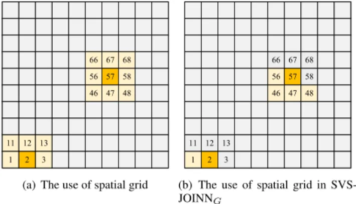
b: SPATIAL GRID
We propose a grid based spatial partition strategy named spatial grid to improve the performance of algorithm. This strategy is to model the two-dimensional spatial area of datasetRas a grid, denoted as G(R) that contains several
Algorithm 2SVS-JOINBAlgorithm
1: INPUT: R is a geo-image dataset sorted by a global ordering8,0V is a textual similarity threshold,0G is
a geographical similarity threshold.
2: OUTPUT:P is the result pairs set.
3: foreachv∈Wdo 4: Lw← ∅; 5: end for 6: foreacho∈Rdo 7: |Pf(I.V)|S← |I.V| − d0V|I.V|e +1; 8: |Pf(I.V)|I ← |I.V| − d 20V 0V+1|I.V|e +1; 9: fori=1 to|Pf(I.V)|Sdo
10: V ←thei-th visual word ino.V;
11: for e(Iˆ,iIˆ) ∈ Lw and GeoSim(I,Iˆ) ≤ 0G and
| ˆo.V| ≥0V|o.V|do 12: ifQualifyPosFilter(I,iI,Iˆ,iIˆ) && QualifySufFilter(I,iI,Iˆ,iIˆ)then 13: I[Iˆ]←I[Iˆ]+1; 14: else 15: I[Iˆ]← −∞; 16: end if 17: end for 18: ifiI ≤ |Pf(I.V)|I then 19: Lw←L∪ {(I,iI)} 20: end if 21: end for 22: Verify(I, I,P); 23: end for 24: return P;
cells, which equals to the geographical similarity threshold 0Gin each dimension. Thus, the area of each cell equals02G.
Clearly, the spatial grid is determined by a spatial visual similarity join with datasetRand threshold0G. To put it in
another way, for a given datasetR, the gridG(R) do not need to pre-compute.
Fig.5(a) shows how to generate candidate pairs by using spatial grid. The number in a cell is the cell id. We assume that a geo-image is located in the cell 57 colored by yellow, denotedC57. To retrieve the candidate pairs (I,Iˆ), just only
theC57 and its eight neighbor cells colored by light yellow
need to be accessed due to the restriction of geographical similarity threshold. Therefore, for one geo-image, we only need to check total nine cells to find its partner to form a candidate pair. If the current accessed cell is near the edge of the grid, such asC2, only six cells should be checked for
candidates searching. Thus, the search space can be reduced significantly by using this strategy. We utilize the spatial similarity filter to find the result from these cells mentioned above.
c: SVS-JOINGALGORITHM
Based on spatial grid method, we develop an extension of SVS-JOINBcalled SVS-JOINGalgorithm. Like SVS-JOINB,
FIGURE 5. An example of spatial grid.
Algorithm 3SVS-JOINGAlgorithm
1: INPUT: R is a geo-image dataset sorted by a global ordering8,0V is the visual similarity threshold,0G is
a geographical similarity threshold.
2: OUTPUT:Pis the result pairs set.
3: G(R)←GridConstructor(R, 0G); 4: foreachCi∈G(R)do 5: M[Ci]←GetJoinCells(G(R),Ci); 6: foreachCj∈G(R)do 7: P←P∪SVS-JOINB(Ci,Cj, 0G, 0V); 8: end for 9: end for 10: return P;
a spatial grid is constructed for the input datasetRas the basic spatial data structure. The geo-images inRare then accessed in the ascending order of their cell id. For each cellCi, this
algorithm will get a cells set denoted asM[Ci], in which the
geo-image will be joined with all of the geo-images inCi.
In M[Ci], the neighbor cells ofCi have smaller id thanCi
itself.
There are some differences between SVS-JOINB and
SVS-JOING. For example, SVS-JOINGalgorithm builds an
inverted index for all cells in the grid, rather than a global index. Therefore, for each visual wordvin the global visual dictionary, every cell has its inverted indexCi.Lw.
Algorithm3demonstrates the process of SVS-JOING
algo-rithm. Similar to SVS-JOINB algorithm, the input consists
of a geo-image dataset R sorted by 8, a visual similarity threshold0V and a geographical similarity threshold0G. The
first step is to build a spatial gridG(R) forR, shown in Line 3. The geo-images are ordered according to cell id and |I.V|. After this step, it traverses theG(R) to search the join cell by cell. For each cellCi, the procedure GetJoinCell(G(R),Ci)
is executed to get the cell setM[Ci]. For all the cellsCj ∈
M[Cj], the algorithm executes SVS-JOINB(Ci,Cj, 0G, 0V)
to return the final results set. It is worth noting that the geo-imageIlocated in each cellCiare checked several times,
that means more buffers need to create to store the cells for later processing.
D. THE QUADTREE BASED GLOBAL INDEX METHOD
To further improve the search efficiency, in this section we propose a novel method to solve the problem of SVS-JOIN based on a global inverted index and quadtree partition strat-egy.
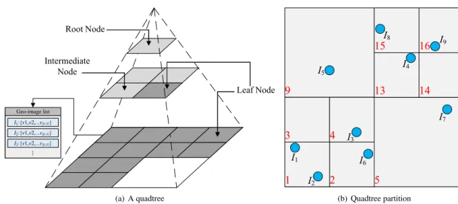
1) QUADTREE PARTITION AND GLOBAL INDEX
a: QUADTREE PARTITION
Quadtree is one of the popular spatial indexing structures used in many applications. It aims to partition a 2-dimensional spa-tial region into 4 subregions in a recursive manner. Fig.6(a) illustrates an example of quadtree that partitions the spatial region intoL levels. Forl-th level, the region is split into 4l equal subregions. Each node of quadtree corresponds to a subregion. The root node of quadtree locate on the 0-th level, which represents the whole spatial region. Four subnodes in 1-level are partitioned from the root node in 0-th level. And the subnodes in 3-level are split from the nodes in 2-level as the same manner. From the Fig.6(a) we can find that there are three colors of nodes. In specific, the light gray nodes are root node and intermediate nodes. The dark gray nodes in any level of the quadtree are the leaf nodes according to the split condition. For each leaf node, there is a list of geo-images in it. In general, the whole spatial region is partitioned into several nodes and the geo-images distribute in these nodes.
Fig. 6(b) shows the partition of the Example 2 by a quadtree. The red color number in quadtree is the node id. Apparently, these 9 geo-images are distributed in the subre-gions. For node 1, denoted asN1, it contains two geo-image
I1andI2. As the number of geo-images inRis really small,
the other nodes contain only one geo-image at most.
b: Z-ORDER CURVE
In this paper, we utilize Z-order curve [91] to encode each node of quadtree according to its partition sequence. As a typical space-filling curve technique, Z-order curve can map multi-dimensional data to one dimension while keeping the spatial position of data unchanged. There is a direct relation-ship between Z-order curve and quadtree. That is, we can utilize the Z-order to sort the data during the quadtree con-struction. That means the path of the node in quadtree can be represented as Z-order curve. Once sorted, the spatial data can either be stored in a binary search tree and used directly [92]. Fig.7(a) demonstrates how to generate the Morton code of a subregion based on spatial partition sequence in a region. According to Z-order curve, we denote these 16 subregions from 0 to 15 in decimal, or from 0000 to 1111 in binary. Fig.7(b) illustrates the Morton code in the quadtree partition of Example2. It is obvious that the 2-dimensional spatial data are mapped to 1-dimensional space. In our solution, we use the code in binary as the node id.
2) SVS-JOINQALGORITHM
Based on the quadtree partition and the global inverted index, we develop a novel algorithm called SVS-JOINQ
FIGURE 6. An example of quadtree partition.
FIGURE 7. An example of Z-order.
Algorithm 4SVS-JOINQAlgorithm
1: INPUT: a geo-image dataset R, a visual similarity threshold0V, a geographical similarity threshold0G. 2: OUTPUT: a result pairs setP.
3: Tquad ←QuadtreeConstructor(R, 0G); 4: Rˆ ←AscSortZ(R); 5: IG←GlobalIndexConstructor(Rˆ, 0V); 6: foreachI ∈ ˆRdo 7: P←P∪JoinSearch(I,IG, 0V, 0G); 8: end for 9: return P;
to solve the spatial visual similarity joins problem effi-ciently. Algorithm4shows the pseudo-code of this algorithm. Algorithm 5 and Algorithm6 demonstrate two key proce-dures applied in SVS-JOINQ. The first step of SVS-JOINQ
is to construct a quadtree by performing the procedure
QuadtreeConstructorin Line 3 to partition the whole spatial region of the input datasetR. In Line 4, the sorting function
AscSortZ(R) is invoked to sort the data in ascending Z-order. After that, the procedureGlobalIndexConstructor(Rˆ, 0V) is
invoked in Line 5 to build the global inverted index for each
Algorithm 5GlobalIndexConstructor(Rˆ,0V)
1: INPUT: a geo-image dataset Rˆ, a visual similarity threshold0V.
2: OUTPUT: a inverted index setIG.
3: Initializing: sort the visual words in descending order of number of non-zero entries;
4: Initializing: Denote the maximum ofw(I.V[i]) for allI ∈ ˆ
Ras maxweight ofi-th visual word;
5: Initializing: Denote the maximum ofw(I.V[i]) from 1 to
mas maxweight ofI.V;
6: Initializing:P← ∅;
7: Initializing:∀ιi∈IG← ∅; 8: Initializing:SV ← ∅; 9: foreachI∈ ˆRdo
10: β ←set of geo-image inI.nodeorI.neighbors;
11: Denote the maximum of I.V[i] for all I ∈ r as maxweighti(r);
12: foreachI.V[i]>0 in ascending order ofido
13: SV ←SV+maxweighti(r)∗I.V[i]; 14: ifSV > 0V then 15: InvertedIndexConstructor(ιi); 16: end if 17: end for 18: end for 19: foreachιj∈IGdo
20: Recordpstart andpend of each node inιj; 21: Record thepIi inιj
22: end for
23: return IG;
visual word according to the visual similarity threshold0V.
When building the inverted index lists for geo-imageI, only the geo-image Iˆ in the neighbor nodes or the same node need to be considered. Then for each inverted indexing list, the algorithm recalls the start position and end position of
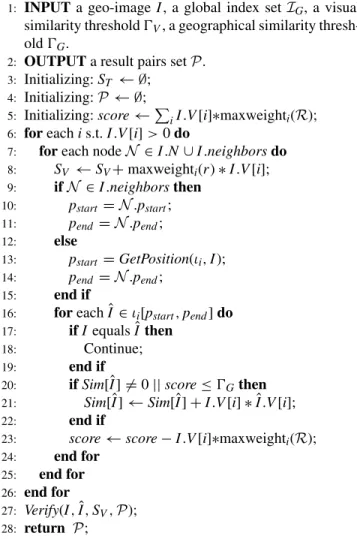
Algorithm 6JoinSearch(I,IG,0G,0V)
1: INPUTa geo-image I, a global index setIG, a visual
similarity threshold0V, a geographical similarity
thresh-old0G.
2: OUTPUTa result pairs setP.
3: Initializing:ST ← ∅; 4: Initializing:P ← ∅;
5: Initializing:score←P
iI.V[i]∗maxweighti(R); 6: foreachis.t.I.V[i]>0do
7: foreach nodeN ∈I.N∪I.neighborsdo
8: SV ←SV+maxweighti(r)∗I.V[i]; 9: ifN ∈I.neighborsthen 10: pstart =N.pstart; 11: pend =N.pend; 12: else 13: pstart =GetPosition(ιi,I); 14: pend =N.pend; 15: end if
16: foreachIˆ∈ιi[pstart,pend]do 17: ifI equalsIˆthen
18: Continue;
19: end if
20: ifSim[Iˆ]6=0||score≤0Gthen
21: Sim[Iˆ]←Sim[ˆI]+I.V[i]∗ ˆI.V[i];
22: end if
23: score←score−I.V[i]∗maxweighti(R); 24: end for
25: end for
26: end for
27: Verify(I,ˆI,SV,P); 28: return P;
each node and the exact position of geo-images for search-ing.JoinSearch(I,IG, 0G, 0V) in Line 7 is invoked to
mea-sure the geographical similarity and visual similarity and then retrieve all the similar geo-image pairs to generate the resultsP.
V. EXPERIMENTS
In this section, we present results of a comprehensive perfor-mance evaluation on real and synthetic geo-image datasets to evaluate the accuracy, efficiency and scalability of the pro-posed approaches. Firstly, we introduce the details of dataset and workload in subsectionV-A. Then in subsectionV-Bwe discuss the results of experiments on two different datasets.
A. DATASET AND WORKLOAD
1) DATASETS
Performance of the proposed methods is evaluated on both real and synthetic spatial and image datasets. The following two datasets are deployed in our experiments.
• Flickr.Real image dataset Flickr is obtained by crawling millions image from the popular photo-sharing platform Flickr(http://www.flickr.com/). To evaluate the scalabil-ity of our proposed algorithm, The dataset size varies
from 100K to 500K. The geo-location information can be obtained from the geo-tag of each image.
• ImageNet. Synthetic dataset ImageNet is obtained
from the largest image dataset ImageNet, which is widely used in image processing and computer vision. it includes 14,197,122 images and 1.2 mil-lion images with SIFT features. We generate Ima-geNet dataset with varying size from 100K to 500K. The geographical information of the images are ran-domly generated from spatial datasets Rtree-Portal (http://www.rtreeportal.org).
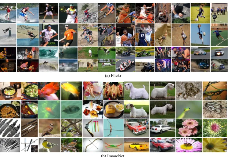
Fig.8shows some example images of these two datasets. Some images selected from Flickr are shown in Fig.8(a), such as the photos of outdoor sports, guitar playing, dogs, etc. The image from ImageNet dataset are shown in Fig.8(b), which belong to many different categories, e.g., fast food, fish, dog, car, snake, flower, etc.
2) WORKLOAD
The geo-image dataset size increases from 100K to 500K; the number of the visual words contained in a geo-image grows from 20 to 100; the geographical similarity threshold 0G and visual similarity threshold0V varies from 0.02 to
0.10 and from 0.5 to 0.9 respectively. By default, The image dataset size, the number of the visual words, the geographical similarity threshold, visual similarity threshold set to300K,
60,0.006,0.7respectively. The default visual representation scheme is AlexNet-BoVW.
All the Experiments are run on a PC with Intel(R) Xeon 2.60GHz dual CPU, 16GB memory and NVIDIA GeForce GTX 1080 GPU running the Ubuntu 16.04 LTS Operation System. The visual feature extraction models (SIFT-BoVW, AlexNet-BoVW, VGGNet-BoVW and GoogLeNet-BoVW) are implemented in Python and all the SVS-JOIN search algo-rithms (SVS-JOINB, SVS-JOING and SVS-JOINQ) in the
experiments are implemented in Java. Note that the quadtree of SVS-JOINQmethod is maintained in memory.
B. PERFORMANCE EVALUATION
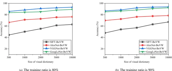
1) COMPARISON BETWEEN VISUAL REPRESENTATION SCHEMES
We compare the search accuracy of four proposed visual representation schemes: SIFT-BoVW, AlexNet-BoVW, VGGNet-BoVW and GoogLeNet-BoVW. As this is the first work to solve the SVS-JOIN problem, we just compare our methods on Flickr and ImageNet datasets.
To evaluate how the dictionary size affect the search accu-racy, we set the size of SIFT/deep visual dictionarys of these four schemes to 500, 1000, 2000, 5000, 10000. The conventional feature representation method, SIFT-BoVW is treated as a baseline, in which the patch size of geo-image is set to 16×16 pixels. For the AlexNet-BoVW method, as mentioned above we use features of the fifth convolutional layer with size of 13×13×256 to generate the visual
dic-FIGURE 8. Some example images of experimental datasets used in our experiment.
FIGURE 9. Accuracy of SIFT-BoVW, AlexNet-BoVW, VGGNet-BoVW and GoogLeNet-BoVW on Flickr Dataset.
tionary. For other two deep feature representation schemes, VGGNet-BoVW and GoogLeNet-BoVW, we utilize features of Conv5_3 layer with size of 14×14×512 and features of inception 4(e) layer with size of 14×14×832 to construct
dictionary respectively. Besides, we choose two training-testing settings for these evaluations, namely (1) training ratio is 80%: the dataset is split into 80% for training and 20% for testing; (2) training ratio is 90%: the dataset is split into 90%
FIGURE 10. Accuracy of SIFT-BoVW, AlexNet-BoVW, VGGNet-BoVW and GoogLeNet-BoVW on ImageNet Dataset.
for training and 10% for testing. The details of experiments are shown as follows.
a: EVALUATION ON FLICKR DATASET
Fig.9 illustrates the comparisons of SIFT-BoVW, AlexNet-BoVW, VGGNet-BoVW and GoogLeNet-BoVW on Flickr dataset under the training ratio of 80% and 90% respec-tively. We can see from the Fig. 9(a) that the accuracy of all of the method creep up with the increase of the size of visual dictionary. Because the larger the visual dictionary, the more details can be represented by visual word model. This directly improves the search accuracy. As the superiority of the VGGNet-16 and GoogLeNet in the image recognition, the perfomances of VGGNet-BoVW and GoogLeNet-BoVW are higher than AlexNet-BoVW and SIFT-BoVW. Since the more semantic concepts information can be captured, these CNN-based approaches can easily combat the conventional opponent for the task of SVS-JOIN search. The accuracy of VGGNet-BoVW is a little higher than GoogLeNet-BoVW, near to 92% at the dictionary size is 10000. When the training ratio is increased to 90%, the performances of these four methods are little better than before. Because enlarging the size of training set can improve the performance of feature representation. However, what hasn’t changed is the best performance of VGGNet-BoVW, which rises gradually with the growth of dictionary size. Similar to the, the accuracy of GoogLeNet-BoVW and AlexNet-BoVW ranked second and third respectively, which are obviously higher than the traditional approach SIFT-BoVW.
b: EVALUATION ON ImageNet DATASET
Fig. 10 demonstrates the results of the experiment between SIFT-BoVW, AlexNet-BoVW, VGGNet-BoVW and GoogLeNet-BoVW on Flickr dataset under the training ratio of 80% and 90% respectively. Under the training ratio of 80%, shown as Fig. 10 (a), all of the methods show a
fluctuating growth as the size of visual dictionary grows. Like the situations on Flickr dataset, VGGNet-BoVW is superior to the opponents, which slowly rises in the internal of [500,5000]. The performance of GoogLeNet-BoVW is the second, which is a bit lower than the former and much higher than AlexNet-BoVW and SIFT-BoVW. The Fig.10(b) shows beyond doubt that the deep CNN based methods are clearly defeat the traditional opponent, SIFT-BoVW, which is exactly the same as before. The accuracy of GoogLeNet-BoVW is very close to VGGNet-BoVW, and the performance of AlexNet-BoVW seems very hard to surpass them. It grad-ually increases to about 76% at the dictionary size is 10000.
2) COMPARISON BETWEEN DIFFERENT SVS-JOIN ALGORITHMS
In the following we evaluate the search efficiency of SVS-JOIN algorithms on Flickr and ImageNet dataset and discuss how the dataset size, number of visual words, geo-graphical and visual similarity threshold affect the system performance. As this work is the first time to evaluate the SVS-JOIN algorithms, we compare the performance of the following methods:
• SVS-JOINB. SVS-JOINBis the technique introduced in
subsectionIV-C.
• SVS-JOING. SVS-JOINGis the technique introduced in
subsectionIV-C.
• SVS-JOINQ. SVS-JOINQis the technique introduced in
subsectionIV-D.
• SVS-JOINS. SVS-JOINS is the technique extended
from the signature-based algorithm in [93]. We modify this existing algorithm by replacing the textual Jaccard measurement with our visual similarity measurement. Besides, we use visual word representation to generate signature.
• SVS-JOINA. SVS-JOINAis a combination of All-Pairs
FIGURE 11. Evaluation on various dataset size on Flickr and ImageNet.
FIGURE 12. Evaluation on the number of visual words on Flickr and ImageNet.
over the dataset. Likewise, we replace the textual simi-larity measurement with the proposed visual simisimi-larity function.
As mentioned above, the default visual representation scheme used in all these approaches is Deep-BoVW (AlexNet-BoVW) in this experiment.
a: EVALUATION ON THE SIZE OF DATASET
We evaluate the effect of the variation of dataset size on Flickr and ImageNet shown in Fig.11. It is obvious that the response time of SVS-JOINB, SVS-JOING, SVS-JOINQ, SVS-JOINS
and SVS-JOINAincrease gradually in Fig.11(a). Specifically,
the performance of SVS-JOINSis the worse than SVS-JOINB
because the search algorithm used in SVS-JOINBis more
effi-cient than SVS-JOINS, which is nearly 30 seconds when the
dataset size is enlarged to 500K. The time cost of SVS-JOING
fluctuate from about 14 second to 23 second, which is higher than SVS-JOINQ because the quadtree and global inverted
index based solution is more efficient. However, it is more efficient than SVS-JOINA due to the use of PPJOIN
algo-rithm. Fig.11(b) illustrates that the evaluation on ImageNet dataset. Similar to the situation on Flickr dataset, the perfor-mance of SVS-JOINQ is the best due to the high efficiency
of quadtree partition strategy. However, with the rising of the dataset size from 100K to 500K, the speed of increment of time cost of SVS-JOINQ is a bit higher than the speed on
Flickr, which might be due to the variety of images. On the other hand, the performance of SVS-JOINBis still worse than
SVS-JOING and SVS-JOINQ since it has no better spatial
index than the others. But SVS-JOINBdefeats SVS-JOIBNS
again, not surprisingly.
b: EVALUATION ON THE NUMBER OF VISUAL WORDS
We evaluate the effect of the number of visual words on Flickr and ImageNet dataset shown in Fig. 12. We can see from Fig.12(a) that the response time of all these five methods
FIGURE 13. Evaluation on the geographical similarity threshold on Flickr and ImageNet.
FIGURE 14. Evaluation on the visual similarity threshold on Flickr and ImageNet.
grow step by step with the increment of number of visual words. Similar to the situation above, the lowest efficient approach is SVS-JOINS that cannot defeat any opponent.
For SVS-JOINB, when the number of visual words is larger
than 40, the growth speed of it is a bit faster. Apparently, the response time of it is high, which is just lower than SVS-JOINS. SVS-JOINQ is the most efficient algorithm
among them on this dataset due to the benefit of quadtree index. As the same visual word representation utilized in these five methods, the impacts of increasing the number of visual words on them are the same, which is reflected in the similar trend. The evaluation on ImageNet dataset is shown in Fig.12(b). Once again, without spatial partition technique and advanced search strategy, the performance of SVS-JOINS
is the worst. In the interval [60,100], the growth speed of SVS-JOINB and SVS-JOINA are bit faster. However, this
situation does not appear in SVS-JOING and SVS-JOINQ.
There is no doubt the performance of SVS-JOINQis the best,
just like the evaluations mentioned above. Thus, once again, the results confirm that the proposed quadtree partition strat-egy is better than the grid partition for SVS-JOIN problem.
c: EVALUATION ON THE GEOGRAPHICAL SIMILARITY THRESHOLD
We evaluate the effect of the spatial similarity threshold on Flickr and ImageNet dataset shown in Fig.13. In Fig.13(a), with the increasing of geographical similarity threshold, the growth rate of response time of all these five algo-rithms are relatively small. It is as expected that SVS-JOINS
approach has the lowest search efficiency from beginning to end. For SVS-JOINB, it shows slight fluctuations of
response time, which is higher than SVS-JOINA, SVS-JOING
and SVS-JOINQ all along because there is no advanced
spatial index technique used in it to boost the efficiency. As explained above, it just considers the filter condition