HAL Id: hal-02302533
https://hal.archives-ouvertes.fr/hal-02302533
Submitted on 9 Oct 2019
HAL
is a multi-disciplinary open access
archive for the deposit and dissemination of
sci-entific research documents, whether they are
pub-lished or not. The documents may come from
teaching and research institutions in France or
abroad, or from public or private research centers.
L’archive ouverte pluridisciplinaire
HAL
, est
destinée au dépôt et à la diffusion de documents
scientifiques de niveau recherche, publiés ou non,
émanant des établissements d’enseignement et de
recherche français ou étrangers, des laboratoires
publics ou privés.
To cite this version:
Özgür Erkent, Christian Wolf, Christian Laugier. End-to-End Learning of Semantic Grid Estimation
Deep Neural Network with Occupancy Grids. Unmanned systems, Word Scientific, 2019, 7 (3),
pp.171-181. �10.1142/S2301385019410036�. �hal-02302533�
Unmanned Systems, Vol. 0, No. 0 (2013) 1–10 c
World Scientific Publishing Company
End-to-End Learning of Semantic Grid Estimation
Deep Neural Network with Occupancy Grids
¨
Ozg¨ur Erkent
a, Christian Wolf
a,b,c, Christian Laugier
a aINRIA, Chroma Team, Rhˆone-Alpes, France.E-mail: [email protected]
bUniversit´e de Lyon, INSA-Lyon, CNRS, LIRIS, F-69621, France. cCITI, INSA-Lyon, F-69621, France.
We propose semantic grid, a spatial 2D map of the environment around an autonomous vehicle consisting of cells which represent the semantic information of the corresponding region such as car, road, vegetation, bikes, etc.It consists of an integration of an occupancy grid, which computes the grid states with a Bayesian filter approach, and semantic segmentation information from monocular RGB images, which is obtained with a deep neural network. The network fuses the information and can be trained in an end-to-end manner. The output of the neural network is refined with a conditional random field. The proposed method is tested in various datasets (KITTI dataset, Inria-Chroma dataset and SYNTHIA) and different deep neural network architectures are compared.
Keywords: Semantic segmentation, occupancy grids, autonomous vehicles, perception
1. Introduction
Autonomous vehicles require precise and accurate perception of the environment to be able to drive safely. Although machine learning methods, in particular deep learning based methods, have provided a significant improvement in the perception skills of intelligent vehicles, perception is still one of the greatest chal-lenges due to varying weather and illumination conditions and the dynamic complexities in the environment such as cars and pedestrians. High-level semantic predictions are made based on low-level sensor data using the high learning capacity of deep neural networks. However, the tremendous number of the pa-rameters in these models makes it difficult to optimize them from low amounts of data. In this study, we fuse the outputs of occupancy grids, which are built by Bayesian methods, with deep networks to estimate the semantic properties of the cells in the occupancy grids. We benefit from both, the high capac-ity of neural networks, and the capabilities of Bayesian methods to handle uncertainties in the system successfully. The spatial map which is composed of grids that contain the semantic in-formation is called as the semantic grid, as an analogy to the occupancy grid.
An Occupancy grid is a 2D spatial map of the environment, where each cell represents the probability of the occupancy state of the environment.1, 2The states provide the information about the occupancy of a cell such as occupied by a static or dynamic object or being free. One of the important features of occupancy grids is that they can represent dense information when the cell size is set appropriately small.
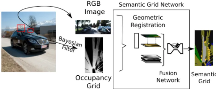
Semantic Grid Occupancy Grid Bayesian Filter Fusion Network RGB Image Geometric Registration
Semantic Grid Network
Fig. 1: A Bayesian filter is applied to obtain the occupancy grid and this information is fused with the semantic information ob-tained from the RGB image via a deep neural network to obtain the semantic grid.
Another attribute of the occupancy grids is that any sen-sor modality can be used such as stereo cameras3or laser range sensors4 since the model is generative, no learning is necessary beyond adapting the observation model of the Bayesian model to the sensor characteristics. However, classical occupancy grids do not contain semantic information about the scene, which would be necessary to make plans about the navigation of the vehicle such as steering to free areas which are labeled as road or other purposes such as planning. To overcome this insufficiency, we propose to use semantic grids which fuse the semantic infor-mation with the occupancy grids.
In this study, we use an approach to fuse the semantic prop-erties of the scene with the occupancy state information. The se-mantic properties are obtained from a monocular RGB image,
which is placed on the vehicle and the occupancy grid is esti-mated by using the laser range sensor (LIDAR) of the vehicle as shown in Fig. 1. The final grid, which contains the seman-tic knowledge of the environment such ascar, pedestrian, veg-etation, road, bike, etc. is called as the semantic grid.5, 6 The method is capable of being used with any semantic segmenta-tion network architecture since it can be trained in an end-to-end manner (including semantic segmentation and sensor fusion, but not the Bayesian estimation module). To be able to refine the final details of the framework, we use conditional random fields (CRFs).7 The proposed framework is composed of three parts: semantic segmentation, occupancy grid estimation via a Bayesian filter and integration of the occupancy grid with the semantically segmented RGB image of the scene. All the sensor information is obtained from the sensors placed on the vehicle.
We compare the performance of different network archi-tectures with various datasets and evaluate the effect of CRFs in semantic grid estimation. We claim the following contributions:
• An end-to-end trainable deep learning method to obtain the semantic grids by integrating the occupancy grids obtained by a Bayesian filter approach and the seman-tically segmented images by using the monocular RGB images of the environment.
• Grid refinement with conditional random fields (CRFs) on the output of the deep network.
• A comparison of the performances of three different se-mantic segmentation network architectures in the pro-posed end-to-end trainable setting.
2. Related Work
The previous work related to semantic grids can be considered in three categories: semantic grids, occupancy grids and finally semantic segmentation. First we will mention the studies related to semantic grids and include the semantic maps in this cate-gory. Next, we will talk about 2D spatial occupancy grids for autonomous vehicles and finally we will present the semantic segmentation studies that are applicable to autonomous vehicles. Integration of maps and semantic information has been the subject of a few studies. Recently, region proposal networks (RPNs)8 have been used to compute semantic segmentations for maps by Tung et. al.9 In,10 the objective is to remove road surfaces and building facades from input point clouds, since it is possible to detect them accurately and rapidly with respect to other structures in the point cloud with a restriction in the scene. These methods suffer from high computational complex-ity since they require a 3D reconstruction of the environment. Other approaches compute the semantic information of the scene from 2D images, which reduces the computation complexity. Dequaire et. al.11 compute such a representation with recurrent neural networks. They do not fuse the RGB data with the LIDAR information in their study. Similar to our work, in ,5Erkent et. al. propose semantic grids. With respect to this work, we perform an end-to-end training and compare the performance of differ-ent semantic segmdiffer-entation network architectures. We also ex-plore the integration of the system with CRFs, which have been shown to provide an increase in the accuracy of the semantic
segmentation in recent methods such as DeepLab v2.12
Classical occupancy grids are 2D spatial maps of the scene containing information about the occupancy states of the grid cells. The Bayesian Occupancy Filter (BOF)13 has gained suc-cess in computing the occupancy grids efficiently by computing the occupancy and dynamic attributes of the grid cells in paral-lel. Further improvement has been provided by the Conditional Monte Carlo Dense Occupancy Tracker (CMCDOT) approach by Rummelhard et al.,2 which introduced four different states and updated only necessary states at the necessary grids. This method can be used in real-time on an autonomous vehicle. Due to its speed and accuracy, we based our grid on CMCDOT in this work.
As aforementioned, an occupancy grid is not sufficient for decision making since the grids do not contain semantic infor-mation on the content. On the other hand, semantic segmentation of RGB images is a well-studied topic. Flat classifiers such as SVM,14 random forests15 and boosting16 were previously used to segment images. The accuracy of segmentation has increased significantly with the arrival of approaches based on deep learn-ing. One of the early works based on deep learning has been per-formed by Farabet et al.17 However, a common problem is that due to cascaded layers, the feature map resolution reduces. The seminal work by Long et. al.18 introduced the widely used con-cept of convolutional encoders and deconvolutional decoders, further enhanced by SegNet19 or U-Net.20CRFs are also com-bined with networks to repair the damaged border edges such as DeepLab.12Grid Networks generalize a large part of the state of the art in a single network and are successful in terms of accu-racy; however, their usage in real-time systems is not feasible at the moment due to their high computational complexity.21
3. Semantic Grid Construction
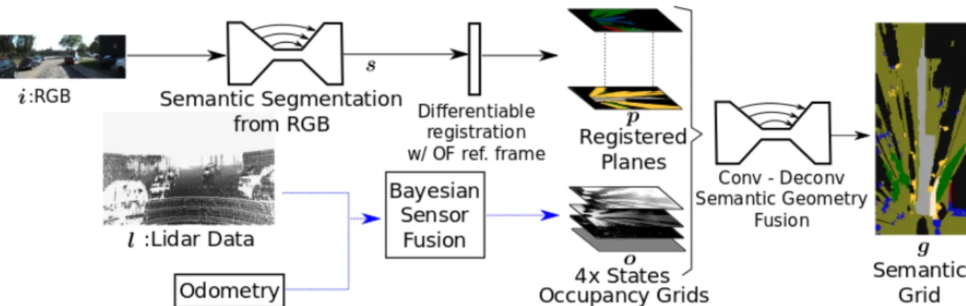
To be able to construct the semantic grid from a top view cen-tered on the vehicle, we fuse the occupancy informationowith the RGB imagei. The objective is to obtain the semantic gridg. An overview of the approach can be seen in Fig. 2.
The pixel values of the image at locationxandyare de-noted asix,y. The values of the semantic grid gcontain class
values denoted byc. All the classes are elements of the alphabet
∀c∈Λ. On the other hand, each cell of the occupancy grid has a probability value for each occupancy state.
In this work, we use two different sensors for the two differ-ent parts of the method: the LIDAR datalis used to compute the (classical non semantic) occupancy grid, and monocular RGB images are used for semantic segmentation, followed by fusion of the two modalities. However, it should be noted that the ap-proach is capable of using any sensor modality to compute the occupancy grid state probabilities.
The LIDAR point cloudslcontain both temporal and spa-tial data. The number of state classes for occupancy is four which are selected as occupied by a static object, occupied by a dynamic object, free area, unknown area. For a cell, the sum of the probabilities of all the four states is one. We use the prob-ability values of the cells when fusing them with the output of the semantically segmented image.
End-to-End Learning of Semantic Grid Estimation Deep Neural Network with Occupancy Grids 3
In the next sections, we explain the semantic segmentation networks used in this study (section 3.1) and the occupancy grid estimation method (section 3.2). The fusion of the occupancy grids with the semantically segmented images will be explained in detail followed by the joint dimensionality reduction and fi-nally the refinement of the output with a CRF will be explained.
3.1. Semantic Segmentation Methods for 2D Images
A semantic segmentation method takes an RGB monocular im-ageias input and estimates the semantic classessfor each pixel. The neural networks are able to estimate the semantic knowl-edge of the pixels by using their high capacity, which translates into a large number of weights. Although these weights give the networks a strong estimation power, they also make the networks require to learn from large datasets. We use pre-trained weights on a large scale dataset ImageNet/ILSVRC .22These weights are fine-tuned on the datasets used. The selected methods have a cer-tain level of runtime/accuracy trade-off. The labels are selected asroad, car, sideways, vegetation, pedestrian, bicycle, building, signage, fenceandunknown.
To keep the resolution of the output same with the input is one of the main difficulties in semantic segmentation meth-ods. This is mainly due to consecutive layers of the network which perform downsampling and pooling. This issue can be resolved by using the methods such as `a trousalgorithm23 or upsampling18and skip connections.20
We use the SegNet variant19 for obtaining semantic infor-mationsfrom monocular RGB images. The accuracy of SegNet is not the highest among other reported results;24 however, its runtime/accuracy trade-off is very favorable. As,18, 20, 25SegNet is an encoder-decoder network. We use the parameters from a previously trained version with a VGG1626 architecture trained for object recognition. The pixels are classified by using a soft-max layer. The labels areroad, car, sideways, vegetation, pedes-trian, bicycle, building, signage, fenceandunknown.
We compare SegNet to two other variants of encoder-decoder networks, namely FCN18and DeepLab v212which uses “atrous convolution” to upsample. We will give more details of these algorithms in the experimental section.
3.2. Occupancy Grid Construction
One of the important components of our approach is the usage of the occupancy grids, for which we use the well-established Bayesian filtering approach. In brief, the occupancy grid is com-puted by using the current observations of the sensors and the previous values of the grid cells. We use the CMCDOT approach which estimates the occupancy states in real-time .2 Although the details of the work can be found in the work of Rummelhard et al. ,2here we will explain CMCDOT briefly.
Each grid cell has probabilities of four corresponding states: being free, being occupied by a static object, being occu-pied by a dynamic object and unknown. The value for the prob-ability of being free implies the probprob-ability of the cell being free of obstacles. A high value does not necessarily mean that the ve-hicle can be steered towards this area since the area can be free,
but it can be a non-drivable area such as vegetation or pedestrian way. The probability value of being occupied by a static object indicates an obstacle. It should be reminded that this can be a potentially mobile object such as a parked car. The dynamically occupied region has a high probability of dynamically occupied region and finally unknown regions indicates the unobserved re-gions. For example the rear region of a car can be unknown due to auto occlusion of the LIDAR by the car itself.
The prediction step uses the probability values of the cells from the previous states. The transformation to the current state from the previous states is carried out by using a transition ma-trix which is pre-defined. In the update, the predicted state prob-abilities are assessed based on a probabilistic sensor (observa-tion) model .27 At the end of the assessment, state distributions are computed. New particles are obtained for new observed ar-eas and previously dynamically occupied arar-eas in the particle re-sampling step. After this last step, the algorithm continues with the prediction. For the interested reader we refer to Rummelhard et al.2
3.3. Fusion of Occupancy and Semantic Information
If obtaining the precise semantic segmentation was possible to-gether with accurate depth information from the RGB image, it would be trivial to integrate the occupancy grid owith the semantic information obtained from the RGB image i. How-ever, depth estimation is inherently error prone, and any er-ror resulting from segmentation accompanied by imperfect and sparse depth information and erroneous explicit calibration er-rors would propagate to the semantic grid. For this reason we do not use a purely geometric approach and we assume that depth information is not available during fusion process. Instead, we propose a method to learn the fusion in an end-to-end training approach.
However, we do not rely on a simple black-box approach for fusion. The fusion process can become sub-optimal if no ge-ometrical constraints are used at all, as the RGB and LIDAR sensors are operating in different coordinate frames. Training a deep network to fully learn this geometric mapping between the semantic view and the 2D bird’s eye view map would require tremendous amount of representative data for different cases. To be able to overcome this issue, we explicitly provide the projec-tive geometric relationships between these two views (epipolar geometry) as hard constraints to the neural network. In partic-ular, we transform the segmented RGB image, which is still in the coordinate frame of the RGB camera, into an intermediate representation aligned with the LIDAR coordinate frame, up to unknown degree of freedom related to the missing depth infor-mation.
To be more precise, we first obtain the probability scores sc,x,yfor each pixel in the semantic viewscfrom the RGB
seg-mentation network.crepresents an individual class andCis the number of semantic classes. We haveC semantic images with probability scores at each pixel. The intermediate representa-tion is organized into height planespc,δ
i, which are obtained for
each semantic viewscwith offsetδi(as shown Figure 3). These
Fig. 2: Overview of the method. i: RGB Image,l: LIDAR data, o: occupancy grids, s: output of the segmentation network, p: registered planes as inner representations,g: semantic grid. The continuous black arrows represent the path on which the parameters are learned jointly end-to-end including the registration process while the blue dotted arrows show the process of the occupancy grid computation.
existsDnumber of planes for classcwherei∈ {1, ..., D}.
Fig. 3: Transformation of the projective semantic view into the intermediate representative planes. As it can be observed, they are chosen to be parallel to the occupancy grid. Cis the num-ber of classes. The colored class labels are used for illustration purposes instead the actual probability scores.
The offset between the consecutive planes is constantd=
||δi−δi−1||. Every point in the intermediate plane has a known
distance to the camera since we have designed the location of the planes; therefore, we can find the transformation between the projective imageiand the intermediate representation planes given that we have the knowledge of the intrinsic and approxi-mate extrinsic calibration parameters of the sensors. We know that the height of a pointzij = δiin an intermediate
represen-tation plane{xji, yji} ∈pc,δ
iis the offset of the plane from the
occupancy grid o. Once we compute the location of the point
{xji, yji, zij}in the intermediate plane with respect to the occu-pancy grid o coordinates, we can find the coordinates of this point in the image coordinate frame by using the transforma-tion oitf from the occupancy grid to the image coordinates as follows: xˆji,yˆji,zˆij,1| = iotfxji, yij, zji,1|. Then, it is straight forward to find the pixel location in the image plane as:
¯ xji ¯ yji 1 =K ˆ xji/zˆij ˆ yij/zˆji 1 (1)
where(¯xji,y¯ij)is the location of the jthpoint in theithplane pc,δi and K is the intrinsic camera calibration matrix for all
classesc∈ {1, ...,C}. For each point in the intermediate plane pc,δ
i,xji,y j i
, there exists a probability score in the semantic view sc,¯xj
i,¯y j i
which is the output of the semantic segmentation layers. One of the objectives of this work is to train the model end to end, i.e. to train the segmentation model SegNet together with the sensor fusion network. This requires the sampling from the segmentation result to the intermediate representation to be differentiable. We resort to a sampling kernel to formulate this transformation for the cellpc,δ
i,xji,y j i to a pixel as pc,δ i,xji,y j i = ¯ H X n=1 ¯ W X m=1 sc,n,mk(xji−m; Φx)k(yji −n; Φy) (2)
where∀i∈ {0, ..., D}for all intermediate planes,c∈ {1, ...,C}
for all classes,j ∈ {1, ..., HW},(H, W)is the height and width of the occupancy grid and( ¯H,W¯)is the size ofs, the semantic view. We prefer to use a bilinear sampling kernel k(.)since it has been shown to be differentiable by Jaderberg et. al.28Ifδi,
the distance between planes, is sufficiently small and the points in the plane is visible in the semantic view projection plane, then at least one of the planes will contain the point with the correct class probability of the corresponding cell in the semantic grid and our model is expected to learn this association between the semantic grid and the occupancy grids and the intermediate rep-resentation planes.
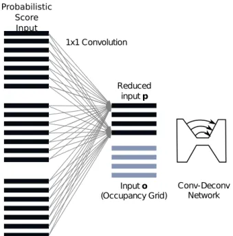
3.4. Joint Dimensionality Reduction and Fusion
The semantic grid outputghas the same spatial dimensions as the input tensors occupancy grid oand the intermediate
repre-End-to-End Learning of Semantic Grid Estimation Deep Neural Network with Occupancy Grids 5
sentation planesp, requiring a resolution preserving neural map-ping. We use convolution-deconvolution networks25 similar to SegNet20for this task, including skip connections.19
The input tensor hasD×C+4planes. 4 planes belong to the probability states of the occupancy grid o, while D×C planes belong to the output of the intermediate representation planes. Each plane represents the probability scores of a seman-tic class for a plane at an offset distance. It is inefficient to learn a mapping from this high dimensional input, which would re-quire a network with a huge capacity with a large amount of pa-rameters. Therefore, we include a dimensional reduction layer, which is jointly trained with fusion. In particular, we use1×1
convolutions to create the effect of a point-wise (stationary) non-linearity with spatially shared parameters. We learn the dimen-sionality reduction and fusion jointly end-to-end as shown in Fig. 4. This reduction layer is expected to reduce the training and inference time while not affecting the estimation accuracy.
Probabilistic Score Input Reduced inputp 1x1 Convolution Inputo (Occupancy Grid) Conv-Deconv Network
Fig. 4: The intermediate plane representation which has a size ofD×Cplanes, is reduced to a lower dimensional tensor before being concatenated with the occupancy grid.
In more detail, the indices of the maximum values after max-pooling in the encoder stage are stored and used by the de-coder of the network during upsampling. The dede-coder part also has the same number of layers as the encoder part. Each layer in the network has a convolution, batch-normalization and ReLu. In the last layer, multi-class softmax is used for classification. We use cross-entropy as the loss.18One of the main differences from the original SegNet architecture is that we are using a re-duced version of convolution-deconvolution network with less number of layers due to memory restrictions. The architecture of this part with the reduced number of layers can be seen in Fig. 5.
Fig. 5: The fusion network architecture. A reduced numbered of layers is used with respect to a standard VGG16 network. The labels are as follows: 1: Convolution + Batch Normalization + ReLU, 2: Max-Pooling, 3: Upsampling, 4: Softmax
3.5. Refinement with Conditional Random Fields
Although convolution-deconvolution method is used to reduce the effect of reduction in resolution, it is still not sufficient for a high quality output. One of the solution offered in semantic seg-mentation of RGB images is to use Conditional Random Fields (CRFs) on the final output image. They generally provide a smoother segmentation with improved labeling since the neigh-boring nodes can be coupled together which reduce the ambigu-ities at the borders of the class pixels.29 We are also evaluating the effect of using CRFs on semantic grids. Since the semantic grids have a different appearance than the RGB image represen-tation, the improvement may not be as effective as using them on RGB images. We are using the fully connected CRF model7 which uses the following energy function:
E(x) =X i φu(xi) + X i<j φp(xi, xj) (3)
i, j ∈ {1, ..., HW}.xi are the grid class labels.φu(xi)is the
unary potential. It is the output of our semantic grid network and contains the distribution over label assignmentxi. The
sec-ond part is the pairwise potentials. It is obtained by combining two parts: φp(xi, xj) =µ(xi, xj)[w1exp(− |ci−cj|2 2σ2 α −|oi−oj| 2 2σ2 β ) +w2exp(− |ci−cj|2 2σ2 γ )] (4) Again,xi, xj are the grid class labels. The first is the bilateral
kernel (a Gaussian appearance kernel) that depends on both the locations of the and the values of the cells. The second ker-nel depends on locations only.σα, σβ, σγ are scale parameters
for bilateral location, bilateral values and location only. Bilat-eral kernel enforces the nearby pixels with similar labels to have similar values which results in smoothening effect, while the second kernel takes the spatial relationship into account. µ(xi, xj) = [xi 6= xj]is the simple label compatibility
different labels. To make decisions about higher complexity re-lations, higher-order potentials are necessary to be deployed, which would increase the computation time of the algorithm. Therefore, we skip to use the higher-order potentials in this study.
4. Experiments
We evaluate the proposed method on data obtained from the sen-sors placed on a vehicle. We create the labels for the bird’s eye view representation since the semantic labeling is generally per-formed in the frontal RGB camera plane of the vehicle. Evalua-tion was performed on three different datasets:
KITTI Dataset — introduced in,30 this dataset has all the ve-hicle position, LIDAR data and RGB data. We use the semantically segmented version of the dataset which is provided by Zhang et. al.31 In this version, the RGB images are semantically labeled at every 10 frames with 10 classes. 142 images are used for learning and 110 images are used for testing. The semantically seg-mented frontal RGB images constitute the main ground truth for this dataset. We use the depth information from the LIDAR data to transform this ground truth into segmented top view semantic grids. To achieve this, we firstly transform the sparse pointclouds ob-tained from LIDAR data into camera frame. After registering the pixels with a depth value, the regis-tered points are back projected into the occupancy grid frame. For the pixels with more than one depth value, we select the depth value that is closest to the image plane since the other one is probably occluded by this pixel. Due to sparseness of the point cloud, errors in calibration of the camera with respect to LIDAR and the errors in the semantic class labeling, the registration process results in faulty labels. We apply some morpho-logical methods on the images and a human observes the final images and further corrects the semantic grid representations if it is necessary. Therefore, finally we obtain a dense semantic grid with reduced errors. If a cell is not labeled in the semantic view by the human, that region is classified as unknown according to its oc-cupancy grid state, such as static, dynamic or free un-known grid cell.
INRIA-Chroma Semantic Grid Dataset — We used 276 la-beled images in 5 different road sequences. The label-ing has been performed in both RGB view and bird’s eye view. Again the vehicle position, LIDAR data and RGB data are available. 146 images are used for train-ing from 3 routes while 130 images are used for testtrain-ing from 2 remaining routes. This is a private dataset ob-tained by Inria-Chroma with the purpose of testing the approach in a real setting.
SYNTHIA Dataset — introduced in,32 thissynthetic dataset consists of a collection of photo-realistic frames with multiple cameras and depth sensors placed on the same location. We use only one pair of camera and depth data. We use two routes of data which was simulated
as Spring season. The depth data is subsampled to re-semble the data to LIDAR laser range sensor which is sparse. It should be denoted that this does not result in LIDAR data, but reduces the amount of depth data. The position information of the vehicle, the extrinsic and intrinsic calibration parameters of the sensors are available. We use the same parameters for our network which is trained end-to-end and the CMCDOT occu-pancy grid. We train on one of the Spring season con-ditions and test our trained model on another Spring condition. We use only the SegNet variant for semantic segmentation layer and we do not use CRF refinement. We detect the following classes,Void, Building, Road, Sidewalk, Fence, Vegetation, Pole, Car, Sign, Lane. Sky, bike, pedestrian and traffic light semantic classes are not detected since they are not visible in the occupancy grid or not present in the simulator for the used se-quence during testing or training.
4.1. Implementation details
The occupancy grid has been calculated with the Conditional Monte Carlo Dense Occupancy Tracker (CMCDOT).2 The width of the grid is 31m, and the length is 71m with a grid size of0.2×0.2m.
We evaluate the method with three different neural back-bone architectures in the semantic segmentation layers as discussed previously in Section. 3.1: SegNet19 , FCN18 and DeepLab v2.12
SegNet19is a type of encoder-decoder network. During en-coding, the downsampling and pooling is applied in between layers which results in the reduction of the resolution. SegNet tries to resolve this problem by keeping the indices from the encoder layer and uses them during upsampling and unpooling process. The encoder part uses the VGG1626 architecture with 13 layers. The decoder part is similar to encoder part and it also has 13 layers. Softmax is not applied and the outputs with the probability scores are fed as inputs to the fusion part of the net-work when this method is used.
FCN18 is a method which first encodes the input and then uses the output of this encoder as an input to fully-connected lay-ers. The initial layers use an architecture similar to VGG16.26A skip architecture is applied where the output of the deep coarse layer is integrated with a shallow one which contains appearance information. Again no softmax is applied and the outputs with the probability scores are fed as inputs to the fusion part of the network when this method is used.
DeepLab v212uses “atrous convolution” to upsample. It is proposed that this approach is capable of solving the resolution problem due to downsampling and pooling via “atrous convolu-tion”. The pre-trained weights are used from ResNet.33 We do not use CRF at this part of the network.
The weights of the initial networks are taken from the pre-trained network ILSVRC/Imagenet22which was trained for clas-sifying images in a large dataset. The learning rate is selected to be1×10−3and momentum0.9. The mini-batch size is 6;
End-to-End Learning of Semantic Grid Estimation Deep Neural Network with Occupancy Grids 7
all training data. The training is stopped after 2000 iterations or when the loss does not change. The number of intermediate rep-resentation planes is selected to beD= 20and we useC = 14
classes.
An important restriction of semantic classification is that the number of class labels and pixel sizes are not balanced in frequency. Some classes may occur much more often than the others which can result in a poor performance for less fre-quent classes. We use themedian frequency balancing34which is shown to be effective in these kind of situations. The ratio of the number of grids to the number of all grids (if the class is available in the grid) is denoted as the frequency of a class f(c). The idea is to balance the classes by using a class weight αc =
mf
f(c)in the loss function.mf is denoted as the median of
the frequencies. Since it had a superior performance, we used class-balancing in all results. The output of the RGB semantic segmentation is not available since we use an end-to-end train-ing and the semantically segmented RGB images are internal representations of our network. Finally, we perform an analysis on the usage of CRFs on the output of our model (Table. 1).
4.2. Evaluation metrics
We use three commonly used measures for evaluation. pixel ac-curacy is the ratio of the number correctly classified grids with respect to the number of all the grids. Class accuracy is the av-erage of the ratio of the accuracy of each class where each class accuracy is computed by finding the number of correctly classi-fied grids with respect to the total number of grids and the mean of intersection over union based on frequency which is the fre-quency weighted average Jaccard Index. Only the grids which have a ground truth label are used for comparison.
4.3. Ablation study
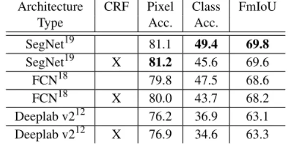
We performed an ablation study on the KITTI dataset. In partic-ular, we tested the effects of different neural backbones can be seen in (Table. 1). The network with the layers similar to Seg-Net19performs the best among others. One of the reasons is that the small number of training samples allow the parameters of SegNet to learn the segmentation better since it has fewer num-ber of parameters. It should be noted that if the training samples have a higher label density and the number of training samples are higher, the results may differ.
Table. 1 also indicates the effect of CRF based refinement. We should note that the improvement is not significant. There-fore we can conclude that the usage of CRF in semantic grids may not be feasible according to our results. Quantitatively, pixel accuracy is increasing slightly; however, the class accuracy is decreasing. This result may be due to the size of the segmented classes. When we use the bird’s eye view to observe the environ-ment, the size of some semantic classes get very small and they are smoothed by the CRF. On the other hand, an advantage can be listed as the removal of the holes in the grids which results in the increase of the overall pixel accuracy.
Table 1: Results with CRF on the KITTI dataset with different neural backbones and with or without CRF based refinement.
Architecture CRF Pixel Class FmIoU Type Acc. Acc.
SegNet19 81.1 49.4 69.8 SegNet19 X 81.2 45.6 69.6 FCN18 79.8 47.5 68.6 FCN18 X 80.0 43.7 68.2 Deeplab v212 76.2 36.9 63.1 Deeplab v212 X 76.9 34.6 63.3
These results are confirmed by the evaluation on the Inria-Chroma dataset (Table. 2). CRF refinement slightly increases the pixel accuracy, while the class accuracy decreases probably due to smoothening of some of the classes in the semantic grid. It should be noted that the usage of higher order potentials may increase the performance at the cost of increased computational complexity.
Table 2: Results with CRF for INRIA-Chroma-Semantic Grid Dataset
Architecture CRF Pixel Class FmIoU Type Acc. Acc.
SegNet 78.6 35.3 65.2 SegNet X 78.9 33.3 65.4
Fig.6 provides qualitative results on scenes selected from both of these two datasets. Same classes with same labels are used for both of the datasets although the training is done sep-arately for both. The RGB images of the scenes are shown in
(a),(e),(i). These are the images taken from the frontal monoc-ular camera of the vehicle. The obtained ground-truths obtained from human labeling for the semantic grid are shown in(b),(f),
(j). We show our predictions in (c), (g),(k) and (o). We also show the effect of CRF refinement in(d),(h),(l). It is interest-ing to observe that we can differentiate between the road and the sidewalk in the semantic grid which has a high probability of free state in occupancy grid without its class for steerability. The vegetation and pedestrians are also detected correctly in the scenes. The slight effect of CRF can be observed in(h)where the false detections introduced by the fusion network is removed by the CRF refinement step.
(a) RGB for scene 1 (b) GT (c) Prediction (d) CRF
(e) RGB for scene 2 (f) GT (g) Prediction (h) CRF
(i) RGB for scene 3 (j) GT (k) Prediction (l) CRF
(m) Colors for labels
Fig. 6: Three scenes with RGB image, ground truth (GT), se-mantic segmentation predictions and results of the CRF refine-ment. Scene 1 and 2 are from KITTI dataset, whereas Scene 3 is from Inria-Chroma dataset.
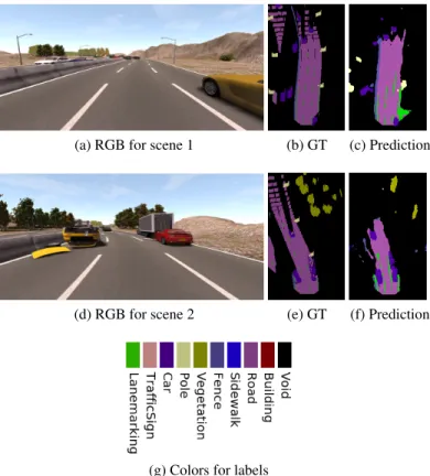
4.4. Validation on synthetic data
We validate the performance on the synthetic SYNTHIA dataset, which provides dense labeling and perfect depth registration. It should be noted that since there is no error in the data related to extrinsic sensor calibrations and semantic labeling of the classes, the error propagation would not occur if we projected the seg-mented images onto the semantic grid. The main error would be the one in the semantic segmentation process. Therefore, we ob-serve the performance of our framework in a setting for which it is not aimed for. We do not perform CRF refinement on synthetic data since it did not improve the performance in the previous datasets.
(a) RGB for scene 1 (b) GT (c) Prediction
(d) RGB for scene 2 (e) GT (f) Prediction
(g) Colors for labels
Fig. 7: Two scenes with RGB image, ground truth (GT), seman-tic and segmentation predictions from SYNTHIA dataset.
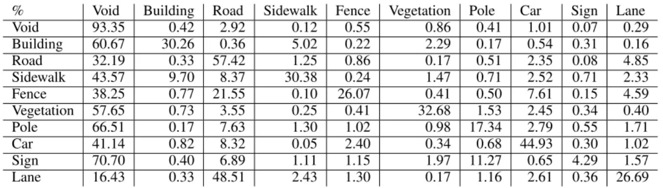
A confusion matrix is given in Table. 3. At each row, the percentage of the classes detected as the corresponding class are shown. For instance, for road, 32.19% of cells are falsely de-tected as void, while 57.42% are correctly dede-tected as road. One of the interesting points is that most of the grid cells are detected void. The accuracy of road and car detection is high. Surpris-ingly, even though the lane markings are very tiny, they have a high correct detection rate. It should be noted that no extra pro-cessing has been made on the lane detection results. In overall, the pixel accuracy is found to be 0.72, the mean class accuracy is 0.36 and the FmIoU is 0.73 which are consistent with results of other datasets.
Fig. 7 provides visualization on several cases, which can shed some light on the nature of these errors. The closer objects tend to give better accuracy. For example, the closer lane mark-ing visibility is better in the semantic grid. However, they are not precisely accurate which results in errors. The poles are also de-tected; however they are larger in size than the actual one. This is probably due to the infrequent appearance of the poles. An-other interesting feature is that since CMCDOT is able to detect the obstacles, even if there is a car which is upside down, and therefore difficult to detect with a standard deep neural network where such images are not provided at training, we can still de-tect it as a car by using our combined framework.
End-to-End Learning of Semantic Grid Estimation Deep Neural Network with Occupancy Grids 9
Table 3: Confusion Matrix for SYNTHIA Dataset
% Void Building Road Sidewalk Fence Vegetation Pole Car Sign Lane
Void 93.35 0.42 2.92 0.12 0.55 0.86 0.41 1.01 0.07 0.29 Building 60.67 30.26 0.36 5.02 0.22 2.29 0.17 0.54 0.31 0.16 Road 32.19 0.33 57.42 1.25 0.86 0.17 0.51 2.35 0.08 4.85 Sidewalk 43.57 9.70 8.37 30.38 0.24 1.47 0.71 2.52 0.71 2.33 Fence 38.25 0.77 21.55 0.10 26.07 0.41 0.50 7.61 0.15 4.59 Vegetation 57.65 0.73 3.55 0.25 0.41 32.68 1.53 2.45 0.34 0.40 Pole 66.51 0.17 7.63 1.30 1.02 0.98 17.34 2.79 0.55 1.71 Car 41.14 0.82 8.32 0.05 2.40 0.34 0.68 44.93 0.30 1.02 Sign 70.70 0.40 6.89 1.11 1.15 1.97 11.27 0.65 4.29 1.57 Lane 16.43 0.33 48.51 2.43 1.30 0.17 1.16 2.61 0.36 26.69 5. Conclusion
In this study, we have shown a method which integrates a Bayesian particle filter with a neural network layer by using a geometric fusion network. This network is shown to work by training end-to-end. We have tested different network architec-tures to be used with our framework and investigated the usage of CRF refinement in the output of our framework. We analyzed our proposal by using several datasets including real data and synthetic data to evaluate the capabilities of our approach.
Acknowledgement
This work was supported by Toyota Motor Europe. We thank Jean-Alix David and J´erˆome Lussereau for their assistance with data collection.
References
[1] H. P. Moravec, Sensor fusion in certainty grids for mobile robots,AI magazine9(2) (1988) p. 61.
[2] L. Rummelhard, A. N`egre and C. Laugier, Conditional monte carlo dense occupancy tracker,ITSC, IEEE (2015), pp. 2485–2490.
[3] M. Perrollaz, J.-D. Yoder, A. Spalanzani and C. Laugier, Using the disparity space to compute occupancy grids from stereo-vision,IROS, IEEE (2010), pp. 2721–2726. [4] J. D. Adarve, M. Perrollaz, A. Makris and C. Laugier,
Computing occupancy grids from multiple sensors using linear opinion pools,ICRA, IEEE (2012), pp. 4074–4079. [5] O. Erkent, C. Wolf, C. Laugier, D. Gonzalez and V. Cano,
Semantic grid estimation with a hybrid bayesian and deep neural network approach,IEEE IROS, (2018), pp. 1–8. [6] O. Erkent, C. Wolf and C. Laugier, Semantic grid
estima-tion with occupancy grids and semantic segmentaestima-tion net-works,ICARV, (2018), pp. 1–8.
[7] P. Krahenbuhl and V. Koltun, Efficient inference in fully connected crfs with gaussian edge potentials,NIPS, (2011).
[8] S. Ren, K. He, R. Girshick and J. Sun, Faster r-cnn: To-wards real-time object detection with region proposal
net-works, Advances in neural information processing sys-tems, (2015), pp. 91–99.
[9] F. Tung and J. J. Little, MF3D: Model-free 3D semantic scene parsing,ICRA, (2017), pp. 4596–4603.
[10] P. Babahajiani, L. Fan, J. K. K¨am¨ar¨ainen and M. Gabbouj, Urban 3D segmentation and modelling from street view images and LiDAR point clouds,Machine Vision and Ap-plications28(7) (2017) 1–16.
[11] J. Dequaire, P. Ondr´uˇska, D. Rao, D. Wang and I. Pos-ner, Deep tracking in the wild: End-to-end tracking us-ing recurrent neural networks, The International Journal of Robotics Research(2017) p. 0278364917710543. [12] L. C. Chen, G. Papandreou, I. Kokkinos, K. Murphy and
A. L. Yuille, Deeplab: Semantic image segmentation with deep convolutional nets, atrous convolution, and fully con-nected crfs,IEEE PAMIPP(99) (2017) 1–1.
[13] C. Cou´e, C. Pradalier, C. Laugier, T. Fraichard and P. Bessi`ere, Bayesian occupancy filtering for multitar-get tracking: an automotive application,The International Journal of Robotics Research25(1) (2006) 19–30. [14] B. Fulkerson, A. Vedaldi and S. Soatto, Class
segmen-tation and object localization with superpixel neighbor-hoods,ICCV, (2009).
[15] M. J. Shotton and R. Cipolla, Semantic texton forests for image categorization and segmentation,CVPR, (2008). [16] J. Shotton, J. Winn, C. Rother and A. Criminisi,
Texton-boost for image understanding: Multi-class object recogni-tion and segmentarecogni-tion by jointly modeling texture, layout, and context,IJCV(2009).
[17] C. Farabet, C. Couprie, L. Najman and Y. LeCun, Learning Hierarchical Features for Scene Labeling,PAMI, (2013). [18] J. Long, E. Shelhamer and T. Darrell, Fully convolutional
networks for semantic segmentation,CVPR, (2015). [19] V. Badrinarayanan, A. Kendall and R. Cipolla, Segnet: A
deep convolutional encoder-decoder architecture for image segmentation,IEEE PAMI39(12) (2017) 2481–2495. [20] O. Ronneberger, P. Fischer and T. Brox, U-net:
Convolu-tional networks for biomedical image segmentation, MIC-CAI, (2015).
[21] D. Fourure, R. Emonet, E. Fromont, D. Muselet, A. Tremeau and C. Wolf, Residual Conv-Deconv Grid Net-work for Semantic Segmentation,BMVC, (2017).
[22] O. Russakovsky, J. Deng, H. Su, J. Krause, S. Satheesh, S. Ma, Z. Huang, A. Karpathy, A. Khosla, M. Bernstein et al., Imagenet large scale visual recognition challenge, IJCV115(3) (2015) 211–252.
[23] F. Yu and V. Koltun, Multi-scale context aggregation by di-lated convolutions,International Conference on Learning Representations (ICLR), (2016).
[24] G. Lin, C. Shen, A. Van Den Hengel and I. Reid, Exploring context with deep structured models for semantic segmen-tation,IEEE PAMI(2017).
[25] H. Noh, S. Hong and B. Han, Learning deconvolution net-work for semantic segmentation,ICCV, (2015), pp. 1520– 1528.
[26] K. Simonyan and A. Zisserman, Very deep convolutional networks for large-scale image recognition,arXiv preprint arXiv:1409.1556(2014).
[27] S. Thrun, W. Burgard and D. Fox, Probabilistic robotics (MIT press, 2005).
[28] M. Jaderberg, K. Simonyan, A. Zisser-man and K. Kavukcuoglu, Spatial transformer networks, NIPS, (2015), pp. 2017–2025.
[29] C. Rother, V. Kolmogorov and A. Blake, Grabcut: Interac-tive foreground extraction using iterated graph cuts,ACM transactions on graphics (TOG),23(3), ACM (2004), pp. 309–314.
[30] A. Geiger, P. Lenz and R. Urtasun, Are we ready for au-tonomous driving? the kitti vision benchmark suite,CVPR, (2012).
[31] R. Zhang, S. A. Candra, K. Vetter and A. Zakhor, Sensor Fusion for Semantic Segmentation of Urban Scenes,ICRA, (2015), pp. 1850–1857.
[32] G. Ros, L. Sellart, J. Materzynska, D. Vazquez and A. M. Lopez, The synthia dataset: A large collection of synthetic images for semantic segmentation of urban scenes, The IEEE Conference on Computer Vision and Pattern Recog-nition (CVPR), (June 2016).
[33] K. He, X. Zhang, S. Ren and J. Sun, Deep residual learning for image recognition,IEEE CVPR, (2016), pp. 770–778. [34] D. Eigen and R. Fergus, Predicting depth, surface normals
and semantic labels with a common multi-scale convolu-tional architecture,ICCV, (2015), pp. 2650–2658.
¨
Ozg ¨ur ERKENTreceived his B.S. degree on
Mechanical Engineering and M.S. degree on Cognitive Science both from Middle East Technical University in 2001 and 2004 respectively and Ph.D. degree from Electrical and Electronics Engineering, Bogazici University in 2013. From 2013 to 2017 he was Researcher at the Innsbruck University. Now he is a re-searcher at Inria, Chroma Team, Rhˆone-Alpes, France.
Christian WOLF is associate professor (Maˆıtre de Conf´erences, HDR) at INSA de Lyon and LIRIS, a CNRS laboratory, since sept. 2005. He is interested in ma-chine learning and computer vision, especially the visual anal-ysis of complex scenes in motion. His work puts an emphasis on modelling complex interactions of a large amount of vari-ables: deep learning, structured models, and graphical models. Since September 2017 he is partially on leave at the chroma work group and the CITI Laboratory, where he is interested in the connections between machine learning and control. He re-ceived his MSc in computer science from TU Vienna, Austria, in 2000, and a PhD in computer science from INSA de Lyon, France, in 2003. In 2012 he obtained the habilitation diploma, also from INSA de Lyon.
Dr. HDR Christian LAUGIERis Research Director at Inria and Scientific Advisor for Probayes SA and Baidu. His current research interests mainly lie in the areas of Autonomous Vehicles, Embedded Perception & Decision-making, and Bayesian Reasoning. He is a member of sev-eral IEEE International Scientific Committees and he has co-organized numerous workshops and major IEEE conferences in the field of Robotics such as IROS, IV, FSR, or ARSO. He also co-edited several books and special issues in high impact Robotics or ITS journals such as IJRR, JFR, RAM, T-ITS or ITSM. He recently brought recognized scientific contributions and patented innovations to the field of Bayesian Perception & Decision-making for Autonomous Robots and Intelligent Vehi-cles. He is IROS Fellow and he is the recipient of several IEEE and conferences awards in the fields of Robotics and Intelligent Vehicles, including the IEEE/RSJ Harashima award 2012. In ad-dition, he has co-founded four start-up companies.