Monetary Policy, Investment and Non-Fundamental Shocks

Full text

(1)

(2) Monetary policy, investment and non-fundamental shocks Fernando Alexandre∗ First draft: October 2002†. Abstract Using a sticky price model with endogenous investment and adjustment costs we analyse the benefits of monetary policy reacting to asset prices, when investment is under the influence of a non-fundamental shock, both for inflation-forecast targeting rules and for Taylor rules. We conclude that in this context there are benefits from reacting to asset prices that result from a more stable output gap, which is the consequence of a much lower volatility in firms’ investment. However, welfare gains depend on the source of asset price movements. Reacting to asset prices when there is a non-fundamental shock to investment stabilises both the asset price and inflation. Words: Investment; Asset Prices; Inflation Targeting; Taylor Rule; Rational Expectations. JEL Classification:. ∗ †. Department of Economics, Birkbeck College and University of Minho (email: falexandre@econ.bbk.ac.uk) The author is extremely grateful to John Driffill, Pedro Bação and other participants in Birkbeck Col-. lege Seminar for helpful comments.The usual disclaimer applies. The author also acknowledges financial support from the Subprograma Ciência e Tecnologia do Segundo Quadro Comunitário de Apoio, grant number PRAXIS/BD/19895/99.. 1.

(3) 1. Introduction. If movements in stock prices reflected only fundamentals, policymakers would not have to pay attention to price volatility per se. However, and at least since the seminal work of Shiller (1981), theoretical and empirical work suggest that fashions and fads, and not only fundamentals, affect stock prices. Additionally, for policymakers to concern with movements in stock prices those non-fundamental movements will have to affect real economic activity. As discussed in Alexandre and Bação (2002) there are three most likely channels by which equity prices impinge on the real economy: households’ wealth effect, Tobin’s q, and the firms’ balance sheet channel. The first channel, the households’ wealth effect, captures the influence of asset prices on households’ wealth and then on aggregate consumption. The second and third channels capture the effect of stock markets on investment (although the balance sheet channel may also apply to consumption). However, empirical studies have not found a strong reliable relation between the stock market and consumption, not giving support to an important role for the wealth effect. Additionally, we concluded that with a wealth effect as estimated in empirical studies there were no significant benefits from reacting to asset prices. We therefore believe that the effects of stock prices on the real economy through its effects on investment and its implications for monetary policy deserve more attention. Investment in fixed capital is crucial for developments in the real economy. Because of its high volatility and weight in industrial economies investment is seen, at least since John Maynard Keynes, as a major determinant of aggregate fluctuations; investment is also the channel by which new technology is introduced in the economy and therefore decisive for long term growth. Periods of expansion in stock markets have been associated with great booms in investment. Examples of that relationship are movements in stock prices and in investment, in the Japanese economy, during the eighties and, in the American economy, during the nineties. The Japanese 225 stock price index Nikkey climbed from 11 543 in January 1985 to 38 916 - an increase of 237% or an average annual growth rate of 27.5%; the S&P 500 stock price index for the American economy climbed from 459 in January 1995 to 1521 in September 2000 - an increase of 231% or an average annual growth rate of 23.5%. For those periods, fixed capital investment increased at a average annual real growth rate of 9%. The role of monetary policy during an asset price run-up has been the subject of discussion among economists and policymakers at least since the 20s and the Great Depression that fol2.

(4) lowed.1 The research on this topic was most increased after the bubble in stock and housing markets in the Japanese economy, in the eighties, and its burst in the nineties, and the potential repetition of those events in the US economy. That reaction by the Fed has now, that the booming market is over and the American economy is on the edge of recession, increased the criticisms on Chairman Alan Greenspan on its easy monetary policy. Critics argue that it had contributed to the development of the stock market bubble and the boom investment that is responsible for part of the now existing excess of capacity in the American economy. In the nineties, the inflation-targeting regime was almost universally accepted as the ideal monetary policy regime and, in their 1999 influential paper, Ben Bernanke and Mark Gertler argue that that regime will always deliver the best result either there is a bubble or not. That is, according to that view, ”monetary policy should not respond to changes in asset prices, except insofar as they signal changes in expected inflation”. Although that view is almost consensual among economists, it has been the subject of some criticisms, notably by Cecchetti et al (2000). One argument against that view was the one, then very prescient, put forward by Olivier Blanchard, in January 2000. In his view, a flexible inflation-targeting regime may not be the best monetary policy strategy to deal with a bubble economy because overvalued stock prices may induce firms to invest more than is justified by fundamentals, with a resulting excess of capital accumulation in the economy. On the same vein, William Poole (2001) discussing the role of asset prices to monetary policy asserts, ”the distorted price signals from the stock market permitted the industry to raise capital easily and cheaply, which certainly contributed to the overexpansion.” In this context, William Dupor (2001) argues that asset prices inflation should be taken into account by policymakers as an indicator of capital overaccumulation. Following this idea, we use a sticky price model with endogenous investment being driven by non-fundamental movements in asset prices to question the potential benefits of monetary policy reacting to asset prices. We assume that equity prices are contaminated by sentiment i.e., deviations from rationality - and that they can distort firms’ investment decisions: managers cannot disentangle sentiment and information about fundamentals what can motivate ’wrong’ investment decisions. In case of a bubble in stock prices it can result in an excess of capital accumulation. In section 2 we briefly discuss the relationship between stock prices and investment. In section 3 we describe the empirical findings on firms’ reaction to investors’ sentiment. In section 4 we present a sticky price model with endogenous investment and adjustment costs and analyse 1. For a description of the issue of monetary policy and asset prices see Alexandre and Bação (2002).. 3.

(5) the benefits of monetary policy reacting to asset prices. Section 5 analyses the dynamics of the system when this is hit by a technology and a non-fundamental shock. Section 6 anlyses the issue of asset price versus inflation stabilization. Section 7 concludes.. 2. The channels of stock prices to investment. As mentioned above, there are strong reasons to believe that stock prices are ’infected by sentiment’. Another question is the extent to which firms should react to it. Blanchard, Rhee and Summers (1993) looking at the effect of market valuations, even if it differs from managers’ assessment of fundamentals, on investment describe the opposite views of Bosworth (1975) and Fisher and Merton (1984). As Bosworth (1975) put it, ”The stock market and investment behaviour are intimately bound together since firms invest to earn profits, and activity in the stock market represents an attempt by investors to evaluate the magnitudes of that stream of profits.” However, Bosworth (1975) argues that managers should ignore the information from the market and base their investment decisions on their own valuation of fundamentals. In that case the market would be a sideshow with no effect on investment decisions. On the other hand, Fischer and Merton (1984) argue that managers should simply consider the stock market valuation and ’explore investor sentiment’. In the authors’ opinion firms in taking their investment decisions should react to stock prices changes, whether or not they coincide with their assessment of fundamentals: firms should follow investor exuberance and invest until the marginal product of capital equals the rate of return he expects. In this case, sentiment, that is, non-fundamental movements in asset prices, affects investment and, therefore, the real economy. Although there is by now enough evidence that stock returns predict investment (Mork et al: 1990) the channels that make that correlation hold are not so evident. The most mentioned channel between stock prices and investment is the Tobin’s q, first presented in Tobin (1969): q is the ratio of the market’s valuation of capital to its replacement cost. For example, an increase in stock prices increases the value of capital relative to the cost of acquiring new capital and thus increases investment demand by firms. However, several studies (see, for example, Summers: 1981; Barro: 90; Blanchard, Rhee and Summers: 1993; and Chirinko: 1993) have shown that q is not a good predictor of investment at least when compared to other variables. Another important channel from which stock prices influences investment is the most emphasised balance sheet channel (see, for example, Bernanke, Gertler and Gilchrist: 1999; and Kiyotaki and Moore: 1995): stock prices affect firms’ net worth and thus their costs of financing, 4.

(6) by its impact on the collateral firms can offer to banks, what affects investment. Mork, Shleifer and Vishny (1990) when revising the different channels from stock prices to investment mention the one that stresses the fact that managers, when making investment decisions, have in the stock market a source of information that may or may not correctly describe future fundamentals. According to this view, the active informant hypothesis, stock prices predict investment because they convey relevant information to managers when deciding on investment. It is arguable that the market does inform managers of firms, which have to take investment decisions, about, for example, the future state of the economy, namely, future aggregate or individual demand. According to Mork et al (1990) the active informant hypothesis is more plausible for the market as a whole in the sense that is more arguable that managers can benefit from stock market signals from the market as a whole than from market signals about their own businesses. However, that information contained in stock prices can accurately, or inaccurately, predict fundamentals. It can inaccurately predict fundamentals because of its inherent unpredictability ”or because stock prices are contaminated by sentiment that managers cannot separate from information about fundamentals” (Mork et al: 1990). In that case, sentiment - that is, the component of stock prices that is not explained by fundamentals - may distort investment decisions through the false signals it transmits to the managers. According to the Mork et al (1990) terminology, in that case, the stock market will be a ’faulty active informant’. Gilchrist and Leahy (2002) mention that, ”Large movements in asset prices tend to be associated with waves of optimism and pessimism about the future”. If there is some irrational exuberance in the stock market driving prices up because investors believe in a New Era economy, as described in Shiller (2000) and as it happened during the 90s with the dotcoms, as recent events seem to confirm, then firms can be ’forced’ to follow that enthusiasm and invest beyond what would be suggested by fundamentals. This excess of optimism or pessimism easily feeds in investment decisions as John Maynard Keynes soon noticed in what he named ’animal spirits’. This result is related to Shiller’s New Era idea: in some periods, often associated with the appearance of a new technology, there is a widespread sense of living in a new age where high economic growth will rest forever. That certainly happened in the American economy during the nineties, and certainly contributed for the euphoria in the stock market and for the high levels of investment. The levels of investment were conspicuously high in the new economy firms2 . 2. In The General Theory, John M. Keynes stressed the role of uncertainty in investment decisions and how. optimistic or pessimistic states - ’animal spirits’ in Keynes’ words - are crucial to firms’ investment decisions. Changes in investment decisions were then seen was one of the main forces driving the cycle.. 5.

(7) Another channel mentioned by Mork et al (1990) for stock prices to influence investment beyond what is predicted by fundamentals is by the pressure it may exert on managers. This stock market pressure hypothesis is similar to the faulty informant hypothesis in the sense that managers can try to extract more information from stock prices than it conveyed about fundamentals. Thus, the result again can be distortion in investment decisions.. 3. Investment and stock prices: empirical evidence. Next we present the results of empirical work that evaluate how stock prices affect investment when firms have the information about fundamentals. A first problem in this literature is that fundamentals are unobservable by the econometrician and therefore a proxy has to be chosen sales and cash flow in Mork et al (1990) and profits or its expected present discounted value as in Blanchard et al (1993) - and that is not independent of the results. Another remark is on the choice of the variable for market valuation, that is, Tobin’s q or the stock price. The use of q can easily result in measurement error problems, given the problems involved in the construction of q, namely, the construction of capital at replacement cost. As we will see, one result of these studies is that stock prices outperform q in explaining investment. Mork et al (1990) regress investment growth - the growth of real capital expenditures excluding acquisitions - on stock returns and the growth in fundamental variables in order to see how important the stock market is after controlling for fundamentals - the growth rates of sales and cash flow. As they put it, they try to answer the following question, ”If managers knew future fundamentals, would orthogonal movements in share price still help predict their investment decisions?” Although they concluded that they could never reject the null hypothesis that investor sentiment does not affect investment through the stock market, their results suggest that it is not the most important factor in explaining investment. For firm-level data they conclude that investor sentiment has a very small explanatory power for investment and they conclude that the ”market may not be a complete sideshow, but nor is it very central”. The same results were achieved from aggregate data leading the authors to conclude, ”The stock market is a sometimes faulty predictor of the future, which does not receive much attention and does not influence aggregate investment”. In his study on the effects of stock prices on investment, Barro (1990) concludes that stock prices are an important determinant of for US investment, especially for long-term samples, and even when he controls for cash flow variables. He also concludes that the stock market 6.

(8) outperforms a standard q-variable in explaining investment. Another important paper on the effects of stock prices on investment is the one by Blanchard, Rhee and Summers (1993). These authors analyse whether investment moves more with the stock market or with fundamentals - using as a proxy, first, the expected present discounted value of the profit rate on information available as of the time of investment, and, then, the profit rate - using time series for the period 1900-1990. When controlling for fundamentals, and especially when they use profits as a proxy, they conclude that market valuation has a limited effect in explaining investment behaviour over the period of analysis and that ”time series evidence strongly rejects the hypothesis that managers simply follow the market valuation”. However, they conclude that stock prices matter with ”an increase of 1% in the market valuation not matched by an increase in fundamentals leads to an increase in investment of 0.45%”. The study of the relationship between stock prices and investment is of great interest during periods of marked deviations of stock prices from fundamentals. This is the case of the 20s and the Great Depression and the crash of 1987, for example. The examination of both periods by Barro (1990) led him to conclude that managers don’t closely follow the market valuation in their investment decisions. Firms invested less during the 20s than implied by market valuation; and after the 1929 crash, investment fell more than the fall in the stock market would suggest. From the analysis of the 1987 crash the conclusion is that firms must have considered other information than market valuation for investment was ”surprisingly strong”. Blanchard et al (1993) reached the same conclusion. Two other periods of marked deviations from the fundamentals are the second half of the 80s in Japan and the 90s in the American economy. Although there are already several works on the events in the Japanese economy, the American economy in the 90s is certainly worth of further research. Looking at the Japanese economy in the 80s, Chirinko and Schaller (2001), using different types of evidence conclude that there was a bubble in the in equity markets and that it affected business fixed investment. The authors first confirm that the stock market boom of the late 80’s coincided with high levels of business fixed investment and that, at the peak in 1989, the funds raised from security issues covered almost 90 percent of the expenditures on business fixed investment by the principal Japanese enterprises, when usually it covers only 30%. Using a non-structural forecasting equation and controlling for other macroeconomic factors that might have affected investment, the authors concluded ”that the investment /capital ratio was about 20 percent higher than predicted by these factors in the late 1980’s, but lower than predicted following the crash”. This evidence is reinforced by the use of orthogonality tests, first used by Hall (1978), and parametric estimates; from these they concluded that the bubble ”boosted 7.

(9) fixed investment by approximately 6-9 percent in the years 1987-89”. Bond and Cummins (2001) Baker, Stein and Wurgler (2002) The overall conclusion of these empirical studies is that market valuation, when considering fundamentals as cash flow and profits, has a role, although a limited one, in the determination of investment decisions. That is, the stock market is not a sideshow; it affects real economic activity.. 4. A model with investment under the influence of sentiment. In presenting the active informant hypothesis Mork et al (90) argue that stock prices influence investment because they convey relevant information - as about future demand - relevant for firms’ decisions. However, as the authors remarke the information about fundamentals in stock prices can be accurate or inaccurate. In the later case the stock market will be a ’faulty active informant’ and may distort investment decisions through false signals to managers. We can therefore ask if in periods of enthusiasm or optimism about the future with stock prices booming and firms induced to invest beyond what fundamentals would imply or, on the other hand, during a wave of pessimism, a crash in stock prices and delays in the implementation of investment projects, there is something monetary policy can do to improve things. That is, does the distortionary effect of the bubble on investment provide an argument, in terms of output and inflation stabilisation, in favour of asset price stabilisation? Dupor (2002) develops a sticky price-imperfect competition model with endogenous capital accumulation and investment adjustment costs and concludes that optimal monetary policy should react to non-fundamental movements in asset prices. His argument is, however, very different from the one put forward by Cecchetti et al (2000). In his model, asset price inflation is relevant for monetary policy not because it signals nominal price inflation but because it can be an indicator of distortions in the capital market. Dupor (2002) determines the optimal policy and concludes that is optimal for the central bank to react to asset prices when a bubble in asset prices generates distortion in investment decisions. According to his results asset price inflation may be relevant for policymakers because it ”may provide an indicator of capital overaccumulation, which cannot be gleaned from examining consumer or price inflation”. The reaction of optimal monetary policy to non-fundamental movements in asset prices stabilises both nominal price inflation and non-fundamental asset price movements. In his model there is a deviation from rational expectations in that firms can ’misestimate the future return to 8.

(10) current capital accumulation’ what affects investment and asset price movements; when firms overestimate them, investment increases and asset prices run-up. In Bernanke and Gertler (1999) model they allow for bubbles in stock prices but its effect on the real economy is transmitted through the balance sheet channel and a wealth effect: investment decisions by firms are based on fundamentals. Thus, in Bernanke and Gertler (1999) non-fundamental movements in asset prices don’t affect investment directly with firms’ investment decisions being based on fundamental q. However in their model the bubble affects firms’ behaviour through its impact on their net worth. In our analysis we use a Dynamic New Keynesian framework with endogenous investment and adjustment costs developed by Casares and McCallum (2000). In this model we include an ad hoc term in the investment equation, that should be seen as a shock to fundamentals, representing a deviation from rationality, that distorts firms’ investment decisions.. 4.1. The model. The model presented in Casares and McCallum (2000) is a model with monopolistic competition and nominal price rigidities to allow for non-neutral effects of monetary policy. In the appendix we provide a more detailed description of the model, with emphasis on the derivation of the equilibrium conditions for consumption and investment. The system is described by the following log linearised around the steady state equations, yt = w1 ct + w2 xt. (1). ct = Et ct+1 − ρ−1 (it − π t ) + βν t 1 δ xt = Et xt+1 + Ω [ΘEt f2t+1 − (it − Et π t+1 ) + ψ t ] + kt 1+δ 1+δ kt+1 = (1 − δ) kt + δkt f2t = f2 (nss , k ss )(yt − kt ). (2) (3) (4) (5). at = ρa at−1 + εat. (6). ȳt = (1 − α)at + αkt. (7). ỹt = yt − ȳt. (8). π t = φ0 Et π t+1 + (1 − φ0 )π t−1 + φ1 ỹt + επt. (9). All variables represent percent deviations around the steady state, except inflation and the interest rate that are in levels. Equations (1) to (8) describe what can be called the IS sector of that economy. Equation (1) is the overall resource constraint with w1 and w2 giving the steady9.

(11) state shares of consumption, ct , and investment, xt , respectively, in total output. Equation (2) is the Euler equation for consumption where it depends positively on its own next period’s expected value and negatively on the real interest rate. Additionally, consumption depends on a preference shock, ν t , that is assumed to follow an AR(1) process. Here, unlike in Alexandre and Bação (2002), we don’t consider any wealth effect of stock prices on consumption because we want to concentrate on the effects of the stock market on investment. Equation (3) is, in Casares and McCallum (2000) words, an ’expectational investment equation’ as investment, xt , depends on its own next period’s expected value. Investment also depends on the difference between the expected return on physical capital, Eft+1 , and the return on the financial asset, rt , that the authors above refer to as the real asset premium. The coefficient of this term, Ω =. 1 (1+δ)ηC1 (xss ,kss ) ,. should be read as the semi-elasticity of investment. relative to the real asset’s premium and depends on the adopted adjustment cost specification and parameterization. The inclusion of costs in installing capital - besides its theoretical justification - results from the fact that, in its absence, capital, the marginal product of capital, and the marginal product of labour are too much volatile than observed in the data. Among the different adjustment cost specification considered in Casares and McCallum (2000) we chose that that makes, as shown in Hayashi (1982), the average value of Tobin’s q equal to its marginal value: that is, total adjustment cost depends not only on the amount of new capital invested but also on the stock of capital, implying constant returns to scale for the production function net of adjustment costs. This specification is of interest to us because, in this case, the marginal value of q, that is a sufficient statistic to determine the level of investment by firms, is equal to the market value of capital. Additionally we include an ad hoc term,ψ t , that should be seen as a shock to fundamentals, representing a deviation from rationality, which results in a distortion in investment decisions. The introduction of that non-fundamental shock represents a deviation from rationality and will imply that firms will sometimes misestimate the gap between the expected return on capital and the real interest rate, what will imply a distortion in investment decisions. The non-fundamental shock will therefore affect investment and asset prices. That shock, when positive, will result in an overestimation of the gap between the expected return on physical capital and the interest rate and will, therefore, stimulate investment beyond what fundamentals suggest. We thus assume that the stock market will be, in this case, a ”faulty active informant” in Mork et al (1990) terminology. Alternatively, it can be interpreted as a misalignment in the fundamental value of capital, which affects investment through a q effect and thus the real economy. We assume that the shock to fundamentals follow an autoregressive process, ψ t = ρf ψ t−1 + εf t . 10.

(12) Equation (4) is the log-linearized form of the investment definition. Equation (5) is the log linear approximation to the marginal product of capital for a Cobb-Douglas production form. Equation (6) describes the process followed by the labour augmenting technology. Equation (7) gives natural output, that is, the output that would prevail if there was no deviation from full price flexibility. Equation (8) defines the output gap as the deviation of output from its natural level. Equation (9) depicts the price-adjustment process - the Phillips curve - in the economy. This specification differs from the New Phillips curve as it includes a backward-looking term for inflation that is believed to match the data more closely. This price adjustment specification is similar to the one adopted by Fuhrer and Moore (1995) and produces both price and inflation inertia. These authors found that this hybrid Phillips curve fits empirically well the USA data. The model is completed with a rule for the monetary policy instrument, the nominal interest rate, and is described in section 4.2. The value of the parameters used in our simulation exercise are as in Casares and McCallum (2000) and are summarised in table 1: Table 1: Parameters’ values ρ. α. δ. φ0. φ1. ρa. ρv. Ω. Θ. w1. w2. 5 0.36 0.025 0.5 0.13 0.95 0.3 2.5 0.03 0.78 0.22 There is no consensus on most values of the parameters in our model. We use a value of 0.13 for the hybrid Phillips curve coefficient on the output gap. This is a higher value than the one used in Casares McCallum (2000), 0.03, and follows the value estimated in Rudebusch (2000) that is thought to be a more reasonable value.. 4.2. Simple policy rules. In this model, monetary policy is implemented through simple monetary policy rules for the nominal interest rate, the instrument of the central bank. All are interest rate rules, and all are simple rules, in that they make the interest rate dependent on the values taken by a small number of key variables. The exclusive use of interest rate rules for policy rests on the evidence that virtually all industrialized countries’ central banks use some short-term (nominal) interest rate as their policy instrument (Walsh, 1998). Simple rules have been widely discussed among academics and in wider discussions about monetary policy. It has been argued that, particularly when they include forward-looking elements, they may have some advantages when compared to optimal rules (Batini and Haldane, 1999). Firstly, simple rules may be more robust in the presence of uncertainty about the actual 11.

(13) model of the economy (as there always is), than optimal rules, which are typically functions of all the predetermined state variables of the model (Taylor, 1999). Secondly, it is argued that simple rules, when including forward-looking variables, can perform almost as well as optimal rules in output and inflation stabilization, and still enhance transparency and make the central bank more accountable, resulting, therefore, in higher credibility.. Of course, because simple rules. do not use all the information available they will not in general be optimal (Black et al, 1997). There is of course a debate as to their descriptive realism. On the one hand, Taylor (1993) has argued that a simple rule — the Taylor rule — was a good description of the Federal Reserve’s interest rate policy, and Clarida, Gali, and Gertler (1998) have argued that the Bundesbank can be represented as having set German interest rates in response to a few key variables. On the other hand, Ryan and Thompson (2000) remark that no central bank actually uses a simple rule. Rudebush and Svensson (1999) argue that central banks use all the information available when setting interest rates. We next briefly describe each of the interest rate rules used in this paper. The symbols used in the following equations are defined as follows: it nominal interest rate; π t inflation rate; yt the output gap; qt fundamental value of capital; ψ t is the non-fundamental shock in the investment equation, described in more detail above in the discussion of the model. All are measured as log deviations from targets except for the nominal interest rate and inflation which is in levels. We consider the inflation-forecast based policy rule where the policy instrument reacts to deviations of inflation from its next period expected value, it = γEt π t+1. (10). Clarida, Gali and Gertler (1998) show that inflation-forecast targeting rules are a good empirical description of the actual behaviour of several central banks since 1979. This class of policy rules mimics the behaviour of inflation targeting regimes, as argued in Alexandre et al (2002) and elsewhere, that is, according to Bernanke and Gertler (1999), the ideal monetary policy strategy whether there is a bubble or not, because price and financial stability are highly complementary and consistent objectives. We then consider the case in which the monetary policy rule reacts not only to deviations of inflation from the target but also to the asset price: it = γ 1 Et π t+1 + γ 2 qt. (11). The behaviour of the system under this policy rule will allow us to assess the arguments of the defenders of a reaction to asset prices when there is some form of irrationality driving their 12.

(14) value. Willam Dupor (2002) found it optimal to react to the asset price because it provides an indicator of capital accumulation, which cannot be identified through the consumer price inflation. We also consider an inflation-forecast targeting policy rule in which the policy instrument instead of reacting to the value of capital itself reacts to its deviations from fundamentals, that is, it reacts directly to the non-fundamental shock: it = γ 1 Et π t+1 + γ 2 ψ t In this rule we assume that central banks can identify misalignments in asset prices and that firms cannot. Additionally, we look at Taylor rules, after Taylor (1993), in which the interest rate reacts to deviations of output and inflation from the target: it = λ1 π t−1 + λ2 yt−1. (12). The main arguments for Taylor rules rest on their simplicity, with the transparency and accountability that the central bank gains thereby, and on the fact that they describe actual monetary policy in several countries since the mid eighties (see, for example, Taylor, 1993). We also consider the case, in which the policy instrument also reacts to the asset price, it = λ1 π t−1 + λ2 yt−1 + λ3 qt. (13). and a policy rule in which the interest rate policy instrument also reacts to the non-fundamental shock, it = λ1 π t + λ2 yt + λ3 ψ t. (14). In choosing the optimised coefficients for the classes of policy rules described above we consider that the policymaker tries to minimise the variance of inflation, output an of the policy instrument. We therefore consider a loss function of the following form, L = V (π t ) + w3 V (yt ) + w4 V (Rt − Rt−1 ). (15). The inclusion of output and inflation in the central bank’s loss function reflects the wide agreement that they represent the most important concerns of policymakers - even inflation targeters as the Bank of England claim that they are not ”inflation nutters”, in Mervyn King words. The inclusion of an interest rate smoothing term in the expected loss reduces volatility. 13.

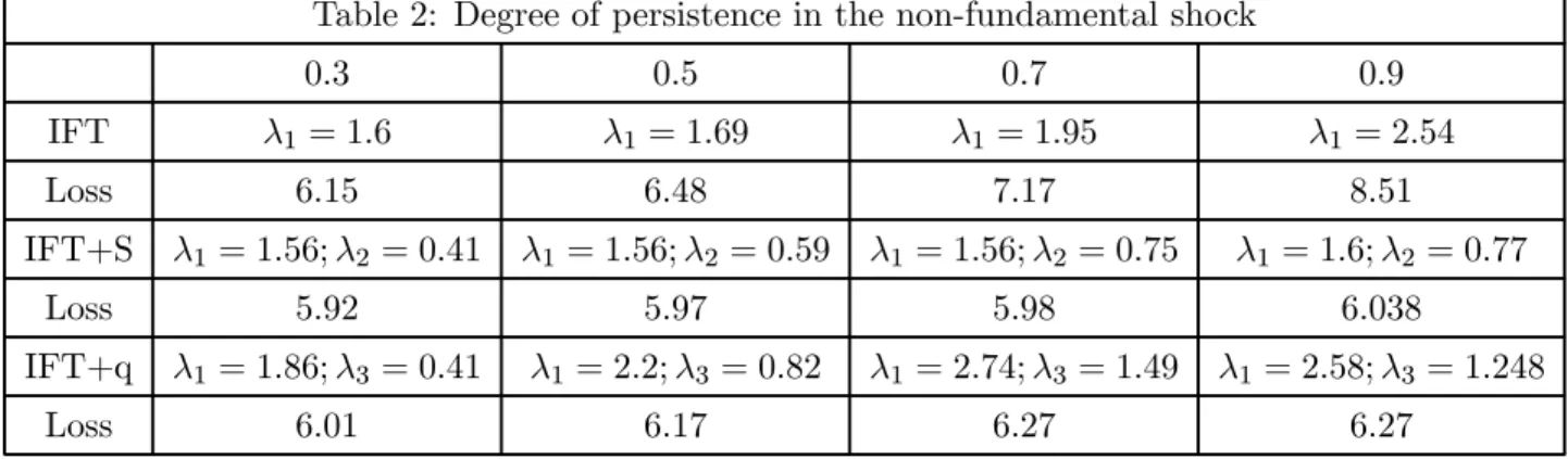
(15) of the policy instrument and is justified, among other reasons, because policymakers are very concerned about financial stability (Mishkin, 1999). This loss can be derived from a microfounded optimal general equilibrium model but without endogenous investment, as shown in Rotemberg and Woodford (1997), as second-order approximation to the utility function of the representative agent. In the baseline simulations the same weight is given to the variance of output and inflation, and half of this weight is given to the variance of the policy instrument. To solve this linear rational expectations model we employed the Schur decomposition as described in Soderlind (1999), after writing the model in the Blanchard-Kahn form.. 4.3. Non-fundamental shock persistence: sensitivity analysis. There is great uncertainty in the volatility of stock prices that is due to fluctuations in the non-fundamental component (Balke, Nathan and Woahar, 2002). The part of the volatility in stock prices that results from the volatility in the non-fundamental component will depend both on the degree of persistence and on the variance of the shock. We therefore do a sensitivity analysis for both parameters of the non-fundamental shock. As in Alexandre and Bação (2002) we start by considering an identity matrix for the variancecovariance matrix of the shocks considered in the model, and compute the optimised coefficients and the loss for different degrees of persistence in the non-fundamental shock in the investment equation. The results for the inflation targeting rule, reacting and not reacting to the nonfundamental shock, are presented in Table 2: Table 2: Degree of persistence in the non-fundamental shock 0.3. 0.5. 0.7. 0.9. IFT. λ1 = 1.6. λ1 = 1.69. λ1 = 1.95. λ1 = 2.54. Loss. 6.15. 6.48. 7.17. 8.51. IFT+S. λ1 = 1.56; λ2 = 0.41. λ1 = 1.56; λ2 = 0.59. λ1 = 1.56; λ2 = 0.75. λ1 = 1.6; λ2 = 0.77. Loss. 5.92. 5.97. 5.98. 6.038. IFT+q. λ1 = 1.86; λ3 = 0.41. λ1 = 2.2; λ3 = 0.82. λ1 = 2.74; λ3 = 1.49. λ1 = 2.58; λ3 = 1.248. Loss. 6.01. 6.17. 6.27. 6.27. As expected the social welfare loss decreases with the degree of persistence of the nonfundamental shock. When we compare the results of reacting and not reacting to the nonfundamental shock we conclude that there is always a welfare benefit from reacting to asset 14.

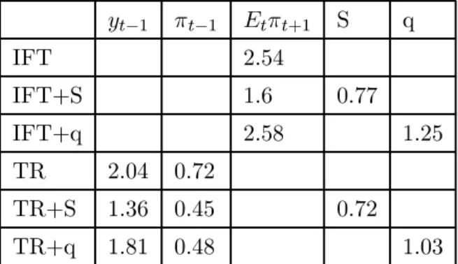
(16) prices and that it increases with the degree of persistence of the shock. The same pattern of results is found for the Taylor rule. Now we do some sensitivity analysis for the variance of the non-fundamental shock. As what is of interest in our study is the variance of the non-fundamental shock relative to the variance of other shocks, we performed our sensitivity analysis for the cases where the variance of the non-fundamental shock is two times and five times the variance of the other shocks, additionally to the case presented above in which the variances of all the shocks in the model are equal to one (see tables in the appendix). We conclude that, for both classes of policy rules, there are significant benefits, in terms of loss, from reacting to both the non-fundamental shock and the asset price itself, with the bulk of it coming from a much more stable output gap. The lower volatility in the output gap results from a conspicuously higher investment stability, as consumption appears to be only slightly volatile. Inflation doesn’t seem to be significantly affected by the variance of the shock. The policy instrument becomes much more volatile as the variance of the non-fundamental shock increases and, for all the cases in analysis, a reaction to both the non-fundamental shock and the fundamental value of capital makes it much more stable. We, therefore, conclude that changes in the variance of the non-fundamental shock appear to result only in differences in the magnitude of the variance of the system, with the quality of the results being unchanged. In the analysis that follows we will concentrate on the case of very high persistence, 0.9, in the non-fundamental shock, that is, a case in which the gap between the expected return on capital and the real interest rate that determines investment deviate for a long period from the fundamentals, and we will consider through our analysis a variance-covariance matrix of shocks equal to the identity matrix.. 4.4. The variance of the system under the different policy rules. The variances of the system are computed as described in Alexandre et al (2002). The optimised coefficients for the different classes of policy rules are given in Table 3: Table 3: Optimal Parameters in Policy Rules. 15.

(17) yt−1. π t−1. Et π t+1. IFT. 2.54. IFT+S. 1.6. IFT+q. 2.58. TR. 2.04. 0.72. TR+S. 1.36. 0.45. TR+q. 1.81. 0.48. S. q. 0.77 1.25 0.72 1.03. Using those coefficients we compute the loss and the variance of the system’s variables for the different policy rules and compare their results, namely, the benefits of reacting either to the asset price itself or to the shock in fundamentals. Table 4 below contains the results. Table 4:. Measures of macroeconomic performance under alternative policy rules. IFT. IFT+S. IFT+q. TR. TR+S. TR+q. V(R). 9.91. 6.24. 6.74. 9.49. 5.8. 7.48. V(K). 46.57. 41.63. 40.92. 47.63. 42.14. 41.57. V(f2 ). 18.93. 16.66. 16.45. 20.41. 17.83. 17.9. V(ȳ). 12.81. 12.16. 11.94. 12.93. 12.19. 11.9. V(y). 16.87. 14.01. 13.76. 16.98. 14.36. 13.7. V(ỹ). 3.82. 1.75. 1.98. 3.88. 2.15. 2.22. V(c). 12.85. 13. 12.87. 12.57. 12.9. 12.5. V(π). 2.79. 2.91. 2.88. 2.96. 2.57. 3.09. V(x). 209.56. 159.51. 157.6. 219.9. 167.34. 166.12. V(Rt − Rt−1 ). 3.79. 2.74. 2.81. 7.08. 3.47. 4.47. V(q). 11.27. 5.73. 5.76. 12.4. 6.72. 6.79. Loss. 8.51. 6.04. 6.27. 10.38. 6.45. 7.54. The first result we should stress is that inflation-forecast targeting rules perform better than Taylor rules in terms of the overall loss. This result comes from a less volatile inflation, output gap and interest rate smoothing term in the inflation-forecast targeting rule. In this case inflation is stabilised without a higher cost in terms of output variability, as it seems to be in Alexandre, Driffill and Spagnolo (2002) and in Alexandre and Bação (2002). The policy instrument is also less volatile in the inflation-forecast targeting rule. The more stable output gap in the inflation-forecast targeting rule case comes from a lower volatility in investment, as the consumption variance is slightly higher than in the Taylor rule. 16.

(18) 4.5. Reacting or not reacting to the shock in fundamentals and to asset prices. According to Bernanke and Gertler (1999) a flexible inflation targeting regime is the most adequate monetary strategy to deal with non-fundamental movements in asset prices. Thus, in their view central banks should adjust the interest rate policy instrument whenever expected inflation deviates from the target and monetary policy should, therefore, respond to movements in asset prices only insofar as they affect expected inflation. Blanchard (2000) criticise the view of Bernanke and Gertler (1999) on how monetary policy should deal with misalignments in asset prices from their fundamental value or, in the more extreme case, with bubbles with the argument that although it stabilises inflation (and the output gap) it will result in an excess of capital accumulation. Assuming that investment is under the influence of both, the real interest rate and the bubble, while consumption is less sensitive to the bubble - in our example consumption is not affected directly by the non-fundamental shock - and that the central bank increases the interest rate, aiming at stabilizing inflation, the result will be a higher decrease in consumption compared to investment, representing a change in the composition of output. The economy would in the end have too much capital and too less consumption. In sum, according to Olivier Blanchard the use of an inflation targeting strategy when there is some sort of irrationality in asset prices will result in excessive capital accumulation because monetary policy is not aggressive enough to pin down its distortionary effect on investment. We therefore look at the benefits of trying to stabilise investment by making the policy instrument react to the deviation of asset prices from fundamentals or to asset prices themselves additionally to deviations of inflation from the target. From the analysis of the table above we conclude that there are gains in terms of welfare from reacting to the non-fundamental shock or to the asset price, in the both the Taylor rule and the inflation-targeting forecast rule. Reacting to the non-fundamental shock delivers the best result in terms of loss welfare. In that case the loss is reduced from 8.51 to 6.04 in the inflation-targeting forecast case, and from 10.38 to 6.45 in the Taylor rule case. The benefits from reacting to the non-fundamental shock and to asset prices result from a more stable output gap, which is the consequence of a more stable investment: the variance of investment is reduced by approximately 25.5% for the inflation-forecast targeting rule and by 24,5% for the Taylor rule, for both the reaction to the non-fundamental shock and to the fundamental value of capital. A reaction to both the non-fundamental shock and to the fundamental value of capital results in very small changes in the variance of inflation and consumption. The results presented above seem therefore to give support to the arguments of Blanchard. 17.

(19) (2000) and other defenders of the ’bubble view’ as, for example, William Dupor (2002) from the University of Pennsylvania, who criticize the view of Bernanke and Gertler (99) that a flexible inflation targeting regime is the most appropriate monetary policy strategy to deal with an asset price run-up whether or not it is driven by non-fundamental movements.. 5. Impulse response functions. In order to better describe the dynamics of the system we present the graphs for the impulse response functions for different shocks with the policy instrument reacting and not reacting to the fundamental value of capital. In appendix 2 we present the graphs for the different policy rules. In order to better contrast the effects of reacting and not reacting to the non-fundamental shock and to the q value, we present both situations in the same graph for the relevant variables. We concentrate on the results for the inflation-forecast targeting policy rule, as it yields the best macroeconomic performance. As we saw above, Cecchetti et al (2000) defend that monetary policy should lean against the wind of significant asset price movements if these disturbances originate in asset markets themselves. Bernanke and Gertler (1999) point the difficulties in identifying the source in asset prices misalignments as one of the main arguments against reacting to asset prices. In Alexandre and Bação (2002) we concluded that the desirability of reacting to asset prices depended on the type of shock hitting the economy. Therefore we analyse the behaviour of the system under the non-fundamental shock and under a shock in the labour-augmenting technology.. 5.1. Non-fundamental shock. The effects of reacting to the non-fundamental shock, in the case of the inflation-targeting forecast rule, that deserve to be stressed are the following. A non-fundamental shock to investment results in an increase in investment and in a decrease in consumption for both policy rules (see fig. 1 and fig. 2). When the economy is under the influence of a positive non-fundamental shock that results in an increase in investment, for the reasons described above, and monetary policy is targeting inflation, investment will still go up and consumption, that is assumed not to depend directly on the fad, will decrease following the increase in the interest rate. This will result in too much capital in the economy. These results support the findings in Dupor (2002), and the arguments of Blanchard (2000), that pursuing an inflation targeting strategy when there is some form of irrationality affecting the value of asset prices will result in too much investment at the cost of a lower consumption with what it implies in terms of a misallocation 18.

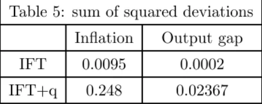
(20) of the resources of the economy. Following the argument of Olivier Blanchard, among others, of reacting to deviations of the expected inflation from the target and, additionally, to deviations from fundamentals results in a smaller departure of investment from its equilibrium value (its initial deviation from equilibrium is reduced by almost 30% when compared to the inflation targeting case) while consumption becomes even more depressed. The higher decrease in consumption when the policy instrument reacts to the asset price results from a higher real interest rate than in the previous case (see fig. 3). However, the output gap and inflation become more stable when the policy instrument reacts to the non-fundamental shock additionally to the deviations of expected inflation from the target (see figs. 4 and 5). Computing the squared deviations from equilibrium for both variables and for both policy rules we get the values in table 4: Table 4: sum of squared deviations Inflation. Output gap. IFT. 1.033. 0.319. IFT+q. 0.0869. 0.0001. From the table the stabilising effects in terms of output gap and inflation from reacting to the asset price are evident.. 5.2. Technology shock. Now we look at the results for the output gap and inflation of reacting to asset prices additionally to reacting to deviations of expected inflation from the target, when the economy is hit by a labour-augmenting technology shock. In this case we conclude that reacting to asset prices when the source of the misalignment is a technology shock makes inflation and the output gap more unstable. Computing the squared deviations from equilibrium for both variables and for both policy rules we get the values in table 5: Table 5: sum of squared deviations Inflation. Output gap. IFT. 0.0095. 0.0002. IFT+q. 0.248. 0.02367. From the values in the table we can see the destabilising effects in terms of output gap and inflation from reacting to the asset price when the economy is hit by a technology shock. The reaction of the policy instrument to the asset price motivates a higher real interest rate (see 19.

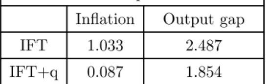
(21) fig. 8), relatively to the situation in which the policy instrument only reacts to deviations of the expected inflation from the target, what results in a higher decrease in the output gap and inflation (see figs. 6 and 7). Decrease in the output gap despite the increase in consumption and investment is because the natural output increases more than actual output in result of the technology shock. We then conclude, as in Alexandre and Bação (2002), that the origin of the shock matters for the decision of whether reacting to asset prices and that, as Cecchetti et al (2000) argue, monetary policy should lean against the wind of significant asset price movements if these disturbances originate in the asset markets themselves.. 6. Asset price and inflation stabilisation. Cecchetti et al (2000) and Mundell (2000) argue that central bankers pursuing price stability will more easily reach that target by reacting to asset prices. In figs. 4 and 8 in the appendix is depicted the reaction of both the inflation and the asset price to a non-fundamental shock when the policy instrument reacts and when it doesn’t react to the asset price in addition to deviations of the expected inflation from the target. From their analysis we can conclude that reacting to asset prices when a non-fundamental shock affects the economy makes inflation and the asset price more stable. The same result can be observed using the sum of squares for inflation and q for both policy rules in table 6, Table 6: sum of squared deviations Inflation. Output gap. IFT. 1.033. 2.487. IFT+q. 0.087. 1.854. Our results seem to support the argument set forth in Cecchetti et al (2000) as both the asset price and inflation seem to be more stable when the policy instrument reacts to asset price in addition to deviations of the expected inflation from the target. However, that result contrasts with the result in Dupor (2002), in the context of a fully optimal policy rule, that finds that asset price stabilisation is achieve at a higher cost in terms of inflation.. 20.

(22) 7. Conclusion. At least since the seminal work of Shiller (1981) theoretical and empirical work suggest that fashions and fads, and not only fundamentals, drive stock prices. Additionally, empirical studies have found evidence that invesment may be affected by a non-fundamental component in asset prices; that is, the impact of asset price movements on investment, either through a q effect or a balance sheet channel effect, may be a most likely channel by which asset prices impinge on the real economy. Periods of expansion in stock markets have been associated with great booms in investment, as in the eighties in the Japanese economy and in the nineties in the American economy. Although high investment rates is of great importance for long term growth, if firms in taking investment decisions are responding to distorted signals from the stock market, the economy can end with too much capital. The consequences of overinvestment as a result of an asset price run-up and the role for monetary policy in this context has been the subject of discussion among economists and policymakers at least since the 20s and the Great Depression that followed. The bubble in the stock and in the housing markets in the Japanese economy, in the eighties, and its burst in the nineties, and the potential repetition of those events in the American economy have raised a wide discussion on what monetary policy can and cannot do to avoid the deranging effects of financial crises to the real economy. Bernanke and Gertler (1999), in their very influencial paper, defend that, because price and financial stability are highly complementary and consistent objectives, when policymakers pursue the former objective they are indirectly contributing to the second. Therefore, according to these authors, a flexible inflation targeting regime is the most adequate monetary strategy to deal with non-fundamental movements in asset prices. That is, according to this monetary strategy central banks should adjust their policy instrument whenever expected inflation deviates from the target and monetary policy should, therefore, respond to movements in asset prices only insofar as they affect expected inflation. This view as been criticised by several authors, among them Olivier Blanchard (2000) and William Dupor (2002), on the argument that an inflation targeting regime, when investment is under the influence of a non-fundamental component in asset prices, will result in an excess of capital accumulation. In this paper we have simulated the effects of different policy rules in a sticky price model wih endogenous investment and adjustment costs in order to analyse the benefits of monetary policy reacting to asset prices when invesment is under the influence of sentiment, that is, under the influence of some form of irrationality. The conclusions of our simulations can be summarised as follows. There are gains in terms of welfare from reacting to the non-fundamental shock and to the. 21.

(23) asset price itself, in both the Taylor rule and the inflation-forecast targeting rule. Benefits from reacting to the non-fundamental shock and to asset prices result from a more stable output gap, which is the consequence of a more stable investment. Therefore, results don’t seem to support the view of Bernanke and Gertler (99) for whom a flexible inflation-targeting regime is the most appropriate monetary policy strategy to deal with asset price run-up whether or not it is driven by non-fundamental movements. We also conclude that, as in Alexandre and Bação (2002), the origin of the shock matters for the decision of whether reacting to asset prices and that, as Cecchetti et al (2000) argue, monetary policy should lean against the wind of significant asset price movements if these disturbances originate in the asset markets themselves; Asset price and inflation seem to be more stable when the policy instrument reacts to asset price in addition to deviations of the expected inflation from the target, when the economy is hit by a non-fundamental shock. This seems to support the argument set forth in Cecchetti et al (2000) that central bankers that pursue price stability will more easily reach that target by reacting to asset prices. However, that result contrasts with the result in Dupor (2002), in the context of a fully optimal policy rule, that finds that asset price stabilisation is achieve at a higher cost in terms of inflation volatility.. References [1] Alexandre, F., John Driffill and Fabio Spagnolo (2002). Inflation Targeting, Exchange Rate Volatility and Policy Coordination. The Manchester School, vol. 70, n 4, pp.546-569 (24). [2] Alexandre, F. and Pedro Bação (2002). Equity Prices and Monetary Policy: An Overview with an Exploratory Model. NIPE Working Paper 03/02, Universidade do Minho and Birkbeck College Working Paper 03/02, Universidade de Londres. [3] Balke, Nathan and Wohar (2002). What drives stock prices? Identifying the determinants of stock prices movements. Review of Economics and Statistics (forthcoming). [4] Barro, Robert J. (1990). The stock market and investment. Review of Financial Studies. 3, 115-132. [5] Batini, N. and A. Haldane (1999). Forward-Looking Rules for Monetary Policy. In John Taylor (ed.), Monetary Policy Rules. Chicago: University of Chicago Press.. 22.

(24) [6] Bernanke, Ben and Mark Gertler (1999). Monetary Policy and Asset Price Volatility, in New Challenges for Monetary Policy, proceedings of the 1999 Jackson Hole Conference, Kansas City, Federal Reserve Bank of Kansas City. [7] Bernanke, Ben, Mark Gertler and Simon Gilchrist (1999). The Financial Accelerator in a Quantitative Business Cycle Frameork. In J. Taylor and M. Woodford (eds.) Handbook of Macroeconomics, North-Holland. [8] Bernanke, B., T. Laubach, F. Mishkin, and A. Posen (1999). Inflation Targeting: Lessons from the International Experience. Princeton University Press: Princeton, New Jersey. [9] Black, R., T. Macklem, and D. Rose (1997). “On Policy Rules for Price Stability”, in Price Stability, Inflation Targets and Monetary Policy. Bank of Canada. [10] Blanchard, Olivier (2000). Bubbles, Liquidity Traps, and Monetary Policy, in Adam Posen (ed.) [11] Blanchard, Olivier J., and Charles Kahn (1980). “The Solution of Linear Difference Models under Rational Expectations”. Econometrica, vol. 48(5), pp. 1305-1311. [12] Blanchard, Olivier, Chanyong Rhee, and Lawrence Summers (1993). The stock market, profir and investment. Quarterly Journal of Economics. 108, 115-136. [13] Bosworth, Barry (1975). The stock market and the economy. Brookings Papers on Economic Activity 2. 257-290. [14] Casares, Miguel and Bennet T. McCallum (2000). An optimising IS-LM framework with endogenous investment. NBER Working Paper # 7908. [15] Cecchetti, Stephen, Hans Genberg, John Lipsky, and Sushil Wadhwani, (2000). Asset Prices and Central Bank Policy. International Center for Monetary and Banking Studies, CEPR. [16] Chirinko, Robert S. (1993). Business fixed investment spending: modelling strategies, empirical results, and policy implications. Journal of Economic Literature. 31, 1875-1911. [17] Chirinko, Robert S. and Huntley Schaller (2001). Business fixed investment and ’bubbles’: the Japanese case. American Economic Review. 91, 663-680. [18] Clarida, R., M. Gertler and J. Gali (1998). “Monetary Policy Rules in Practice: Some International Evidence”. European Economic Review, 42, 1033-1067. 23.

(25) [19] Dupor, William (2002). Nominal price versus asset price stabilization. Paper presented at the CEPR Annual Workshop on Asset Prices and Monetary Policy at the Bank of Finland. [20] Estrella, Arturo, and Jeffrey C. Fuhrer (1998). “Dynamic Inconsistencies: Counterfactual Implications of a Class of Rational Expectations Models”. Federal Reserve Bank of Boston, July. [21] Fischer, Stanley and R. C. Merton (1984). Macroeconomics and Finance: the role of the stock market. Carnegie Rochester Conference Series on Public Policy. XXI (1984), 57-108. [22] Fuhrer, Jeffrey C., and George R. Moore (1995). “Inflation Persistence”. Quarterly Journal of Economics. vol. 110, pp. 127-159. [23] Hamilton, James D. (1994). Time Series Analysis. Princeton University Press. [24] Hayashi, Fumio (1982). Tobin’s Marginal and Average q: a Neoclassical Interpretation. Econometrica. 50, 213-224. [25] Kiyotaki, N. and Moore (1995). Credit Cycles. Journal of Politcal Economy. 105, 211-48. [26] McCallum, Bennett T., Nelson, Edward (1999a). “Performance of operational policy rules in an estimated semi-classical structural model”. in John Taylor (ed.), Monetary Policy Rules. University of Chicago Press. [27] McCallum, Bennett T., and Edward Nelson (1999b). “An Optimising IS-LM Specification for Monetary Policy and Business Cycle Analysis”. Journal of Money, Credit and Banking. 31. [28] Mishkin, F. (1999). “Comment”, in John Taylor (ed), Monetary Policy Rules. University of Chicago Press: Chicago. [29] Morck, Randall, Robert Vishny, and Andrei Shleifer (1990). The stock market and investment: Is the market a sideshow?. Brookings Papers on Economic Activity 2. 157-215. [30] Poole, William (2001). What Role for Asset Prices in Monetary Policy? Speech delivered at Bradley University, Peoria, Illinois, 5 September. [31] Rotemberg, Julio J. and Michael Woodford (1999). Interest Rate Rules in an Estimated Sticky Price Model. In John Taylor (ed.), Monetary Policy Rules. University of Chicago Press. 24.

(26) [32] Rudebusch, Glenn D. (2000). ”Assessing Nominal Income Rules for Monetary Policy with Model and Data Uncertainty”. Federal Reserve Bank of San Francisco, October. [33] Rudebusch, G., and Lars Svensson (1999). Policy Rules for Inflation Targeting. In John Taylor (ed.), Monetary Policy Rules. University of Chicago Press. [34] Shiller, Robert (1981). Do Stock Prices Move Too Much to Be Justified by Subsequent Changes in Dividends?”. American Economic Review. 81, 421-436. [35] Shiller, Robert (2000). Irrational Exuberance. Princeton University Press. [36] Smets, Frank (1997). “Financial Asset Prices and Monetary Policy: Theory and Evidence”. CEPR Working Paper No. 1751. [37] Soderlind, Paul (1999). ”Solution and estimation of RE macromodels with optimal policy”. European Economic Review. 43, 813-823. [38] Summers (1981). [39] Temple, Jonathan (2002). An Assessment of the New Economy. CEPR Discussion Paper. [40] Taylor, John B. (1993). “Discretion vs. Policy Rules in Practice”. Carnegie-Rochester Conference Series on Public Policy. 39, 195-214. [41] Taylor, John B. (ed.) (1999). Monetary Policy Rules. University of Chicago Press. [42] Tobin, James (1969). A General Equilibrium Approach to Monetary Theory. Journal of Money, Credit and Banking. 1, 15-29. [43] Walsh, Carl E. (1998). Monetary Theory and Policy. MIT Press. [44] Woodford, Michael (1999). ”Optimal Monetary Policy Inertia”. NBER Working Paper No. 7261.. 8. Appendix 1. Casares and McCallum (2000) consider an economy populated by a large number of householdsfirms. The representative household-firm seeks at time t to maximise the following intertemporal utility function, separable in consumption and labour, Et. ∞ X. j=0. ³. β j U ct+j , mt+j , υ t+j , ξ t+j 25. ´. (16).

(27) Where β ∈(0,1) is the household’s discount factor. Households consume many goods and the. aggregate ct , the household’s consumption during t, therefore represents a Dixit-Stiglitz (1977) index representing the number of bundles consumed. Each household-firm produces its differentiated good using a Cobb-Douglas technology, yt = (at nt )1−α ktα. (17). where a is a labour-augmenting technology, n is the labour input and K the stock of capital held at the beginning of t. The demand for the household-firm’s differentiated output is given by, YtA. Ã. Pt PtA. !−θ. (18). With YtA the aggregate demand, P the money price of the household-firm’s product, and PtA the aggregate price level. The household inelastically supplies one unit of labour per period to a labour market from which household-firms purchase labour inputs at the real wage rate of wt. Gross investment, xt , is defined as, xt = kt+1 − (1 − δ)kt. (19). where δ is the depreciation rate of capital. The realization of investment implies adjustment costs of the type, xη+1 t (20) ktη where total adjustment cost depends not only on the amount of new capital invested but C(xt , kt ) = κ. also on the stock of capital. With this specification of adjustment costs the production function net of adjustment costs exhibits constant returns to scale. Additionally, this specification makes the average value of Tobin’s q equal to its marginal value, as shown in Hayashi (1982). There is also a market for one-period government bonds, bt+1 , on which the real rate of interest is rt , where (1 + rt )−1 is the real purchase price of a bond that is redeemed for one unit of output in the next period. The household’s budget constraint at t is thus given by, YtA. Ã. Pt PtA. !1−θ. − C(xt , kt ) = ct + kt+1−(1−δ)kt +mt −. 1 1 +wt (nt −1)+ 1+r bt+1 −bt 1+π t t. (21). From the household-firm’s first-order optimality conditions they obtain the log-linear approximation around the steady state in the paper. 26.

(28) non-fundamental shock effect on investment 7 6 5 4. X(t) IFT. 3. X(t) IFT+q. 2 1. Figure 1:. 9. Appendix 2. 27. 61. 56. 51. 46. 41. 36. 31. 26. 21. 16. 11. 6. 1. 0.

(29) non-fundamental shock effect on consumption 0.4 0.2 61. 56. 51. 46. 41. 36. 31. 26. 21. 16. 11. 6. -0.2. 1. 0 -0.4. C(t) IFT. -0.6. C(t) IFT+q. -0.8 -1 -1.2 -1.4. Figure 2:. non-fundamental shock effect on the real interest rate. r IFT. Figure 3:. 28. 61. 56. 51. 46. 41. 36. 31. 26. 21. 16. 11. 6. r IFT+q. 1. 0.9 0.8 0.7 0.6 0.5 0.4 0.3 0.2 0.1 0 -0.1.

(30) non-fundamental shock effect on inflation 0.4 0.35 0.3 0.25 0.2. P(t) IFT P(t) IFT+q. 0.15 0.1 0.05 61. 56. 51. 46. 41. 36. 31. 26. 21. 16. 11. 6. -0.05. 1. 0. Figure 4:. non-fundamental shock effect on output gap 0.6 0.5 0.4 0.3. Ygap(t) IFT. 0.2. Ygap(t) IFT+q. 0.1. Figure 5:. 29. 61. 56. 51. 46. 41. 36. 31. 26. 21. 16. 11. -0.1. 6. 1. 0.

(31) technology shock effect on inflation 0.04 0.02 61. 56. 51. 46. 41. 36. 31. 26. 21. 16. 11. 6. -0.02. 1. 0 -0.04. P(t) IFT. -0.06. P(t) IFT+q. -0.08 -0.1 -0.12 -0.14 -0.16. Figure 6:. technology shock effect on output gap 0.02 61. 56. 51. 46. 41. 36. 31. 26. 21. 16. 11. -0.02. 6. 1. 0. -0.04 Ygap IFT. -0.06. Ygap IFT+q. -0.08 -0.1 -0.12 -0.14. Figure 7:. 30.

(32) technology shock effect on the real interest rate 0.08 0.06 0.04 r ift+q. 0.02. r ift 61. 56. 51. 46. 41. 36. 31. 26. 21. 16. 11. 6. 1. 0 -0.02 -0.04. Figure 8:. non-fundamental shock effect on q 1 0.8 0.6 q IFT. 0.4. q IFT+q. 0.2. -0.2. Figure 9:. 31. 61. 56. 51. 46. 41. 36. 31. 26. 21. 16. 11. 6. 1. 0.

(33) IFT policy rule 7 6. 61. 57. 53. 49. 45. -1. 41. q 37. 0 33. R 29. 1 25. Ygap. 21. 2. 17. X(t+1). 13. 3. 9. P(t+1). 5. C(t+1). 4. 1. 5. -2. Figure 10:. IFT+q policy rule 5 4 C(t+1). 3. P(t+1). 2. X(t+1). 1. Ygap R. -2. Figure 11:. 32. 61. 57. 53. 49. 45. 41. 37. 33. 29. 25. 21. 17. 9. 13. -1. 5. 1. 0. q.

(34)

No results found