Procedia Economics and Finance 30 ( 2015 ) 175 – 186
2212-5671 © 2015 Published by Elsevier B.V. This is an open access article under the CC BY-NC-ND license (http://creativecommons.org/licenses/by-nc-nd/4.0/).
Peer-review under responsibility of IISES-International Institute for Social and Economics Sciences. doi: 10.1016/S2212-5671(15)01281-2
ScienceDirect
3rd Economics & Finance Conference, Rome, Italy, April 14-17, 2015 and 4th Economics &
Finance Conference, London, UK, August 25-28, 2015
The Financial Channel in International Trade
Marta Arespa Castello
a, Diego Gruber
ba Universitat de Barcelona, Gran Via de les Corts Catalanes, 585, Barcelona, Spain b Kernel Analytics, Barcelona, Spain
Abstract
Existent literature is by no means conclusive on the effects of trade finance on trade and the economy. We propose a suitable framework to explore the linkages between international trade and finance based on an international real business cycle model where firms require external finance to import and can be financially constrained. We find that credit shocks do affect the dynamic properties of the economy and they have the potential to cause significant deviations in trade and economic performance. The trade-to-GDP ratio falls following a negative credit shock, as the shock reduces the capability of firms to purchase foreign intermediate goods, thereby reducing efficiency and production. However, it forces a demand substitution towards domestic intermediate goods that limits GDP deterioration. We also find that financially developed countries trade more, are richer and more stable in terms of GDP and consumption, consistence with the empirical evidence. Finally, the model sheds light on persistent contradictions between theoretical business-cycle and their empirical counterparts, namely, the consumption/output anomaly and the volatility of consumption, imports and terms of trade relative to GDP.
© 2015 The Authors. Published by Elsevier B.V.
Peer-review under responsibility of IISES-International Institute for Social and Economics Sciences.
Keywords: Trade finance; credit constraint; great trade collapse; RBC
1.Introduction
We refer to trade finance as either a) one of the mechanisms provided by financial institutions and governments to facilitate international trade activities, or b) an agreement whereby a customer can purchase goods on account, paying the supplier at a later date
.
When trade occurs across borders, sellers require either cash-in-advance payments or formal guarantees to cover themselves from the possibility of insolvency of their buyers. Importers are usually forced to turn to loans or letters of credit to satisfy exporter requirements before having their orders shipped. Most of these contracts are provided by financial institutions and require some form of collateral.© 2015 Published by Elsevier B.V. This is an open access article under the CC BY-NC-ND license (http://creativecommons.org/licenses/by-nc-nd/4.0/).
Trade finance is an extremely important piece of the international trade mechanism; estimates find that around 90% of international trade relies on some form of credit (Auboin, 2009). Since the "great trade collapse”, a large number
of studies has been devoted to clarifying the reasons why this episode occurred. In spite of these efforts, there is still little consensus on the effects of trade finance on macroeconomic variables and, specifically, on international trade performance.
We make a theoretical contribution to this debate within the framework of an International Real Business Cycle (IRBC) model. We propose a dynamic, quantitative, micro-founded macroeconomic model that builds on the standard model of IRBC proposed by (Backus, et al., 1992) (BKK). We introduce an additional requirement for importers, who must borrow proportionally to the value of the goods they wish to import. This feature enables us to shed some light on the role of credit in international trade performance.
Our model provides some relevant improvements over standard IRBC models. Indeed, imports are more volatile than GDP, our quantitative analysis does not suffer from the consumption/output anomaly (i.e., GDP cross-country correlation is larger than consumption cross-country correlation, as in the data), and the volatilities of consumption, imports, and terms of trade relative to GDP are close to those in recent US data. The latter is a property that, as far as we know, required the introduction of non-standard preferences into the model of IRBCs (Raffo, 2008). The financially constrained economy produces negative correlations for net exports and terms of trade with national output. These correlations are found to be positive in standard IRBC models (and in our non-constrained economy), opposite to data. Using a counterfactual analysis we test the macroeconomic effects of alterations in the availability of finance to importers. Compared to a productivity shock of the same size, we find that trade finance does not appear to have a large effect on the behavior of macroeconomic aggregates over the business cycle. However, recent empirical literature show that, indeed, credit shocks account for a large share of the fluctuations of macro-magnitudes, as large as productivity shocks, suggesting that volatility is, indeed, much larger (See, for instance, (Helbling, et al., 2011) and (Hristov, et al., 2012)). A negative credit shock reduces the ability of a producer to use foreign inputs, thereby reducing efficiency, which negatively affects aggregate production. However it also stimulates demand for domestic goods, making them more expensive and harder to come by in foreign markets and reducing exports as well. The net effect on the trade balance is positive, which together with higher demand for domestic goods from constrained importers alleviates the fall in GDP. Hence trade falls faster than GDP in our model following a credit shock. However, unless the variance of credit shocks is much larger than that of productivity shocks, these effects appear to be small in comparison to the effects of productivity shocks, which remain the main drivers of business cycles in our model.
Section 2 presents the model setup and defines the equilibrium of the theoretical economy. Section 3 presents a number of international real-business cycle statistics. We use these numbers to calibrate the model and test its numerical properties. Section 4 contains our main results. Section 5 concludes.
2.The model economy
There are two countries. We denote foreign country variables by an asterisk. Countries are identical except for the stream of productivity shocks they receive. A country consists of four types of agents: Infinitely lived households, the ultimate holders of savings and debt in the model. Final-good firms put together a basket of domestically produced intermediate goods; their output is a final good that can be used for consumption or the accumulation of capital by households. Final goods are sold domestically in perfectly competitive markets. Intermediate good firms operate in a monopolistically competitive setting. They use a fixed amount of labor each period to combine domestic and foreign inputs and manufacture their goods. The amount of foreign inputs they use in production is limited by how much they can borrow to finance their imports. How much they produce depends also on their productivity level, which is affected by a random productivity shock. Production inputs are bought from domestic and foreign input producers, who combine capital and labor in their production process. They can sell their products in domestic markets or export to foreign intermediate good producers.
Financial intermediaries are not explicitly modeled in this paper.* We assume competitive financial intermediaries
channel household savings to intermediate good producers, who require financial support to access to imported input goods. Default is never an optimal choice for borrowers. Household savings are pooled across countries. This allows for unbalanced trade in the model.
2.1.Households
Each country has a mass 1 of identical households. Their utility at each period is given by a strictly concave function
u(ct,1-nt), where ct is consumption and nt the fraction of the time household members spend at work. Furthermore,
they choose how much they invest in new capital ( it ) and how much they lend to importers ( st ). There is a small cost
of holding savings in the form of credit to importers equal to థଶݏ௧ିଵଶ .†
Household earnings come from the salaries they perceive for the amount of time they spend at work ( wt ), from the
share of profits they receive from intermediate good firms ( πt ), the interest they are paid on their savings ( rt ), and
the rents that accrue to them from input producers who rent the capital they own ( Rt ). Hence, the budget constraint
for each period is
ܿ௧ ݅௧ ݏ௧
థ ଶݏ௧ିଵ
ଶ ݓ
௧݊௧ ߨ௧ ݏ௧ିଵሺͳ ݎ௧ሻ ܭ௧ିଵܴ௧ǡ ݐǤ (1)
Physical capital is subject to depreciation at rate δ every period. Following (Backus & Crucini, 2000), physical capital formation is subject to adjustment costs, which are captured by a function Ψ(ڄ), which satisfies Ψ >0 , Ψ '>0 , and Ψ ''<0 . Capital evolves according to
Kt = (1- δ) Kt-1 + Ψ (it /Kt -1) Kt-1 , (2)
We use Ψ ( i/k )=(i/k ) ψ , ψא ( 0,1 ) , so investment is described by the change in capital stocks as follows: it = (
Kt/ Kt-1 -( 1- δ ) ) 1/ψ Kt -1. If households discount utility from future periods at rate β, optimizing behavior is described
by the following problem:
൛ǡǡ௦ǡൟసబಮ σ ߚ௧ݑሺܿ ௧ǡ ͳ െ ݊௧ሻ ஶ ௧ୀ (3) s.t. (1) and (2)
Letting u(c,1-n) = [cμ. (1-n )1- μ]θ /θ , the marginal utilities of consumption and labor are given by ݑ ǡ௧ൌ
ߤܿ௧ఏఓିଵሺͳ െ ݊௧ሻఏሺଵିఓሻǡ ݑǡ௧ൌ െሺͳ െ ߤሻܿ௧ఏఓሺͳ െ ݊௧ሻఏሺଵିఓሻିଵ.
2.2.Final-good firms
Final good firms are homogeneous, act as price takers and make zero profit. Their production function is ܻ௧ ൌ ቀ ݀ǡ௧ఙ݆݀
ଵ
ቁ
ଵ ఙൗ
, where dj,t denotes their demand of intermediate good j. Profits are given by ς ൌ ܻ௧ ௧െ ݀ଵ ǡ௧ǡ௧݆݀ .
Maximizing profits gives their optimal demand of each variety of intermediate goods:
݀ǡ௧ൌ ܻ௧ǡ௧
భ
షభ (4)
* For a model that explicitly models trade finance see (Ahn, 2011)
†† This cost serves for the purpose of determining the steady-state value of the asset position in a zero-order approximation without the need of
taking second-order approximations and ensuring stationarity. See (Benigno, 2009) and (Heathcote & Perri, 2002) for detailed discussions. It does not have any other implication for our results.
2.3.Intermediate-good firms (importers)
Each country has a mass 1 of firms producing differentiated, non-tradable goods. These firms operate in a monopolistic competition setting. Productivity is given by a random shock z t common to all firms. Production takes
place according to the function ܨǡ௧ൌ ݖ௧݄ǡ௧ఈݔǡ௧ଵିఈǡ ߙ א ሺͲǡͳሻ, where hj,t represents the demand of domestic inputs and
xj,t the demand of imported inputs of firm j . Firms pay a fixed cost (Q units) of labor to operate every period. Profits
for the intermediate good producer are given by
ߨǡ௧ൌ ǡ௧݀ǡ௧െ ܲ௧݄Ǥ௧െ ሺͳ ݎ௧ሻܲ௧כݔǡ௧െ ܳݓ௧ (5)
where input prices are denoted by Pt and Pt*, while the intermediate good's market price is pj,t. The firm must
borrow in order to buy imported inputs and therefore pays an interest rt over their total cost. Since imports are bought
on credit they are subject to a trade credit constraint. We think of the degree ߟ to which contracts can be enforced as summarizing the average quality of enforcement in a given economy. The financial intermediary behaves competitively. A credit constraint states that it must be individually rational for the managers to repay their loan. When they abide by the contract, managers receive their net income. When they default, they economize on the payment they owe the intermediary but lose fraction ߟ of the resulting resources. i.e. ߨǡ௧ ሺͳ െ ߟሻൣߨǡ௧ ሺͳ ݎ௧ሻܲ௧כݔǡ௧൧, which implies
ߟሺǡ௧݀ǡ௧െ ܲ௧݄ǡ௧െ ܳݓ௧ሻ ሺͳ ߟሻሺͳ ݎ௧ሻܲ௧כݔǡ௧ǡ (6)
where ߟ ൌଵିఎఎ . Suppose the firm has already chosen a price pj,t inducing demand dj,t. Taking them as given, the
combination of domestic and foreign inputs that minimize the cost of satisfying this demand is given by
ೕǡǡ௫ೕǡܲ௧݄ǡ௧ ሺͳ ݎ௧ሻܲ௧ כݔ ǡ௧ (7) s.t. ݖ௧݄ǡ௧ఈݔǡ௧ଵିఈൌ ݀ǡ௧ǡ ܽ݊݀ߟ൫ǡ௧݀ǡ௧െ ܲ௧݄ǡ௧െ ܳݓ௧൯ ሺͳ ߟሻሺͳ ݎ௧ሻܲ௧כݔǡ௧Ǥ Kuhn-Tucker conditions (KTCs) hj,t = λj,txj,t, whereߣǡ௧ؠଵିఈఈ ൬
ଵିకೕǡఎିకೕǡ
ଵିకೕǡఎ ൰
ሺଵାሻכ
And ߞ௧ and ߦ௧ are the
Lagrangian multipliers of the KTCs. By the first constraint then:
ݔǡ௧ൌ
ௗೕǡ
௭ఒೕǡഀ (8)
We assume intermediate good firms know demand functions (4) and (8) and set their prices accordingly by solving the following profit maximization problem:
ೕǡ ൬ǡ௧െ ௭ఒೕǡഀషభെ ሺͳ ݎ௧ሻ כ ௭ఒೕǡഀ൰ ܻ௧ǡ௧ భ షభെ ܳݓ ௧Ǥ (9)
The solution to this problem is given by
ǡ௧ൌఙ௭ଵ
ఒೕǡഀ ൫ߣǡ௧ܲ௧ ሺͳ ݎ௧ሻܲ௧
2.4.Input producers (exporters)
Each country has a mass 1 of identical input good firms with technologies operating in a perfectly competitive environment. Their technology uses capital (kt) and labor (lt) to generate output ft: ݂௧ ൌ ݇௧ఊ݈௧ଵିఊǡ ߛ א ሺͲǡͳሻǡ an input
producer seeks to solve the following optimization problem:
ǡ ܲ௧݂௧െ ݓ௧݈௧െ ܴ௧݇௧ (11)
The usual FOCs areܲ௧݂ǡ௧ൌ ߛܲ௧ሺሻఊିଵൌ ܴ௧ǡ ܽ݊݀ܲ௧݂ǡ௧ൌ ሺͳ െ ߛሻܲ௧ቀቁ ఊ
ൌ ݓ௧, which together imply an
optimal capital-labor ratio equal to
ൌ ఊ ଵିఊǤ ௪ ோ. 2.5.Equilibrium
This economy is said to be in equilibrium if every period, given a state of the economy (z, z*) and prices P , R , r , and w. Functions c(ڄ) , i(ڄ) , and s(ڄ)solve the household’s problem (3), given prices pj, demand functions dj solve final
good firm problem (5) and their profits are equal to zero. hj, xj and pj are the same for all j and they solve the
intermediate good firm problem (6) and (9). Demands of labor and capital l and k solve the maximization problem of input producers (11) and they have zero profits. Good markets clear: c+i=Y , dj =Fj, and f=h+x*; labor markets clear:
l+Q=n; capital markets clear: k=K; financial markets clear: s+ s*= P*x+Px*; and no-Ponzi-scheme conditions hold. This model has no analytical solution.
3.Quantitative exercise
3.1.Calibration
We shall understand real GDP as the sum of private consumption, investment and exports minus imports: GDPt=ct+it+Pxt*-P*xt , and we refer to net exports as the result of the trade balance divided by GDP, i.e., nxt=(Pxt*
-P*xt)/GDPt , where P and P * are steady state values or constant prices for the model and the data respectively. Terms
of trade refer to the ratio of import and export prices, tott=Pt*/Pt, while the real exchange rate refers to the ratio in the
price level of intermediate goods, rert=pt*/pt. The model is calibrated to match features of the US economy over the
1973-2010 period. We set η=0.57, which is the baseline value used by [ (Amaral & Quintin, 2010)] to match the ratio of financial intermediation to GDP in US.‡§The shock process has the usual form, ݈݃ ቂݖ௧
ݖ௧כቃ ൌ ܣ݈݃ ቂ
ݖ௧ିଵ
ݖ௧ିଵכ ቃ ቂ ߳௧ ߳௧כቃ
where ሺ߳௧ǡ ߳௧כሻ is a vector of i.i.d. shocks. The covariance matrix of these shocks as well as the parameters in the
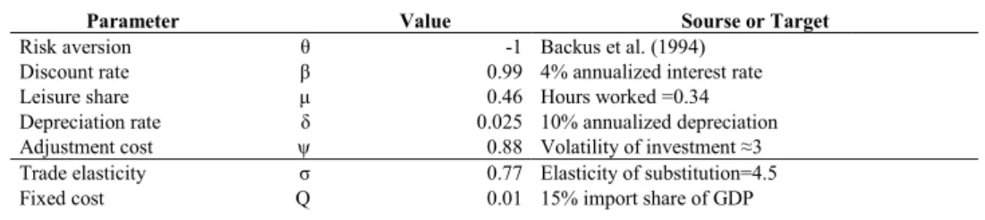
transition matrix A are set after the values estimated by (Heathcote & Perri, 2002). The complete parametrization of the model is given in Table 1.
Table 1: Benchmark parameter values.
Parameter Value Sourse or Target
Risk aversion θ -1 Backus et al. (1994)
Discount rate β 0.99 4% annualized interest rate
Leisure share μ 0.46 Hours worked =0.34
Depreciation rate δ 0.025 10% annualized depreciation
Adjustment cost ψ 0.88 Volatility of investment ≈3
Trade elasticity σ 0.77 Elasticity of substitution=4.5
Fixed cost Q 0.01 15% import share of GDP
‡Simulation results do not change significantly for different values of φ and Q, even if they are set to 0.
§ We performed a robustness test for the results in Table 2 and in the figures using different η . All the qualitative results are robust for a wide
Capital share ϒ 0.41 22% investment share of GDP
Home bias α 0.75 Volatility of imports ε(2,3)
Cost of saving φ 0.01 Mandelman et al. (2011)
Shock process Heathcote and Perri (2002)
Transition matrix Heathcote and Perri (2002)
3.2.Simulation
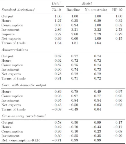
The baseline model does a good job at explaining some of the discrepancies between standard international real business cycle models and the data.**
Excessive consumption smoothness is one such common problem that goes away. (Raffo, 2008), (Raffo, 2010) suggests introducing an alternative specification of household preferences to increase consumption volatility.†† Our
model, however, is capable of generating consumption that is as volatile as in the data with standard preferences. The volatility of imports is about two and a half times as large as the volatility of output, an improvement over standard models, which typically imply lower import volatility than output volatility. The volatility of terms of trade is larger than that of output and quite close in magnitude to what we observe in the data. Auto-correlations of the series in the model are very similar to those in the data as are domestic correlations.
Our mechanism works as follows: when a positive productivity shock hits the economy, households have more income left after consumption. They decide to allocate these savings between importers that need to finance international purchases and input producers (serving both domestic and foreign markets) that need to finance capital. In any case, the extra resources make international trade cheaper: savings devoted to finance imports reduce the total cost of imported goods and savings used to finance exporters capital allow them to produce inputs at a lower cost, becoming more attractive to foreign customers.
The correlation between output and the terms of trade is another common puzzle of international RBC models. Looking at long time series this correlation is typically negative
( (Mendoza, 1995), (Kehoe & Ruhl, 2008)),‡‡while the standard models predict a positive correlation. Our model
predicts a strong negative correlation, a sign consistent with data. The same occurs with the correlation between net exports and domestic output, which is negative in the data and in our simulations but positive in standard RBC models. The latter three features of our results are specific of the financially constrained economy. They are not supported by
the unconstrained version showed in Column “No constraint”.
Another interesting result is that the cross-country correlation of output is stronger than that of consumption, as in the data. This is typically not the case in the literature: (Backus, et al., 1994) dub this the “consumption/output anomaly”. Recall that only national households can invest in national capital. This capital restriction prevents agents from sharing domestic risk further and explains the low cross-country correlation of consumption.§§ The
non-constrained economy shows larger international correlations both for consumption and output. This occurs thank to the existence of firms all over the world that exert a larger demand-pull effect via unconstrained imports, which enhance the transmission of shocks.
** We ran fifty 300-period simulations of this economy, subjected to productivity shocks, and took the log of each series (except for net exports, which may be negative) and used a Hodrick-Prescott filter for quarterly data to remove their trends. We then averaged results from all fifty simulations. Table 2 presents these averages compared to their data counterparts, which have also been logged and HP-filtered as needed for comparison and with results in (Heathcote & Perri, 2002).
†† GHH preferences, as introduced by [ (Greenwood, et al., 1988)], have the property that the marginal rate of substitution between consumption
and leisure is independent of the consumption level within the period, which implies that there is no income effect on labor supply and hours worked respond more strongly to changes in productivity. Although this generates volatility of consumption more in line with the data, the unresponsiveness of labor supply to changes in consumption levels appears to be empirically troublesome.
‡‡ (Mendoza, 1995) §§ See (Olivero, 2010)
ܣ ൌ ቂ ͲǤͻͲǤͲʹͷ ͲǤͲʹͷͲǤͻቃ
Table 2. Simulation results
To what extent do these changes depend on the presence of a credit constraint? We run a modified version of the model that removes condition (6). Importers can buy from foreign firms as much as they can afford and households trade one period non-contingent assets that allow for unbalanced trade, so that s=-s*. The model uses the previous
calibration. Results are in the column “No constraint” of Table 2. When the constraint exists and is binding,
intermediate firms would like to use a larger share of foreign inputs. With a positive productivity shock intermediate firms are able to increase their imports with the resources freed by the lower cost of domestic inputs. As a consequence, net exports decrease with output. After the shock, both countries increase the demand for the cheaper input. Foreign intermediate goods firms, which were more constrained before the shock, redirect part of their demand towards the cheaper input. As a result, P * decreases sufficiently to see a reduction in the terms of trade, which have a countercyclical behavior. Which features of the model make the quantity anomaly disappear? Column “HP 2002” of
Table 2 reports the results for the bond economy in (Heathcote & Perri, 2002). The comparison between their model and ours hints us the answer.*** Their model is suitable to be compared with our no-constraint economy because it
only differs in two relevant features: they have perfect competition for intermediate good producers, which combine
***Be aware that for a reliable quantitative comparison with “HP 2002” we should calibrate the No-constraint version to match actual data. However, we prefer to keep the same calibration used in our baseline model to observe the implications of having the credit constraint or not.
inputs in a CES, while we have monopolistic competition and combine inputs in a Cobb-Douglas. A productivity shock in the Home country causes a milder response in terms of output when competition is monopolistic. This causes a smaller change in relative prices and keeps a larger correlation between cross-country outputs. Moreover, with Cobb-Douglas preferences in consumption, Home and Foreign inputs are in the limit between substitutes and complements, while in a CES, it depends on the selected elasticity of substitution. Any change in the relative use of inputs changes their relative price proportionally with a Cobb-Douglas, but not with a CES. Although some of the differences to the standard international RBC model stem from other characteristics of our model, having a credit constraint allows us to evaluate the effects of changing conditions in financial markets to both the amount as well as the dynamic properties of trade. This is what we do in the next section.
4.How trade finance affects trade
4.1.Effects of a temporary credit shock
In our model, household savings are the crucial source of credit availability determining the volume of trade attainable in this economy. The level of development of the financial system in a country and the strength of its institutions are captured by the parameter η . However, η can also capture changes in risk positions taken by the financial intermediaries. Hence, a larger η may represent both a better developed financial market and a higher level of confidence of banks on loan-repayment possibilities. In order to evaluate the effects of temporary credit shocks we need to add a second source of uncertainty in our model. We shall assume that the credit tightness parameter η is now time dependent with mean ߟҧ; and a random component bt so that ߟ௧ൌ ߟҧܾ௧ the shock process is now ݈݃ ൦ ݖ௧ ݖ௧כ ܾ௧ ܾ௧כ ൪ ൌ ܣ݈݃ ൦ ݖ௧ିଵ ݖ௧ିଵכ ܾ௧ିଵ ܾ௧ିଵכ ൪ ൦ ߳௭ǡ௧ ߳௭ǡ௧כ ߳ǡ௧ ߳ǡ௧כ
൪ There are no reliable time-series on trade finance from which to estimate A and the covariance matrix of the shocks. Therefore, we consider and compare different scenarios and lay out their properties. As a benchmark case, we set all correlations and spillovers between financial and technology shocks to zero. Considering that financial shock transmission across borders has been shown to be a very relevant phenomenon among modern capitalist economies in recent history, we allow for a positive international correlation between trade credit shocks,ܿݎݎሺ߳ǡ ߳כሻ ൌ ͲǤͲ The standard deviation for the financial shock as well as its persistence are initially set
equal to those for the productivity shock.
We now proceed to explore a tightening of 1% in trade credit. Continuous lines in Figure 1 show the impulse responses for the benchmark case. GDP initially increases and then falls below its steady state value for the rest of the transition. The reason is related to the change in the composition of demand by intermediate good producers. When the financial constraint tightens, firms must reduce their demand for imports. They substitute foreign inputs by relatively more expensive national products, pushing domestic production up and, hence, improving GDP. Households lose (at least partially) one of their saving alternatives -the finance of imports-, so they devote more resources to the remaining option -investment in capital-. Foreign input producers lose part of the demand and reduce prices, Pt*.
However, Home input producers reduce their prices further. The upsurge in investment increases capital accumulation just after the shock. This makes it cheaper, generates a substitution from labor to capital and reduces the cost of production of the input and, therefore, its price. As a consequence, TOT increases (deteriorates).
This leads to a fall in exports and, as a consequence, in national GDP. Both imports and exports over GDP are below the steady state during the transition. However, the negative effect of the financial tightening on imports is much larger than on exports, so net exports over GDP improve. The interest rate reduces also because intermediate firms demand less financial resources. On the other hand, the tightening in the financial constraint affects productivity: firms are forced to choose a less efficient mix of domestic and foreign inputs due to the restriction. The obvious consequence is the increase of intermediate goods prices, which damage consumption. Under the current parametrization, the positive effect described above dominates the negative initially. However after a few periods, investment collapse and the initial surge in GDP disappears.
Fig. 1. Change in macroeconomic aggregates following a financial shock for varying levels of financial shock persistence.
The dashed lines in the impulse-response figures above show that the balance between positive and negative effects on macroeconomic aggregates crucially depends on the level of financial shock persistence. When persistence is low the surge in demand for domestic goods is much more short-lived, and therefore increases in investment in anticipation of this surge are too weak to counteract the negative effects of credit-tightening on productivity and exports. Figure 2 illustrates what happens if international correlations drop to 0.50. This change affects the magnitude but not the shape of the response. In the benchmark case, since the shock is transmitted abroad more forcefully, foreign firms find it more difficult to finance imports and hence exports fall significantly more than in the case of milder spillovers. With lower transmission of financial shocks effects over GDP and other macroeconomic aggregates are much milder. We reach virtually the same conclusions if we compare economies with different levels of financial spillovers.
Fig. 2. Change in macroeconomic aggregates following a financial shock for varying levels of international correlations.
Our results are robust to changes in the correlation between financial and technology shocks. If these are different from zero, only the magnitude of the shocks is affected. A positive correlation accentuates the negative effects of a financial shock on productivity, as there will be a loss in efficiency due to a less desirable mix of foreign and domestic inputs and a downgrade in the technology used to combine them. Finally, we compare credit shocks and technology shocks in Figure 3. Both shocks have the same variance, and except for the case of GDP and investment, both have effects in the same direction. The most striking difference is in the magnitude of them, as credit shock effects appear to be much weaker. This explains why the introduction of credit shocks appears to make little difference. However, evidence by (Helbling, et al., 2011) show our result does not imply they are unimportant. Their variance decomposition show credit shocks contribute as much to fluctuations.
Fig. 3. Comparing credit and technology shocks.
Finally, we run a comparative statics analysis of a change in the financial situation of an economy. The qualitative consequences of a permanent tightening in η are the following: A more constrained financial market reduces GDP in the steady state. This result is supported by several papers showing a positive link between financial development and economic growth (See (Levine, 2005) and (Papaioannou, 2008)for a complete survey on the issue.). Imports, on the other hand, decline more than GDP, moving from a 12% to 8% when η changes from .57 to .37, which is approximately the 5% decrease experienced by US real imports over real GDP ratio from its peak to its valley in the recent crisis. When we isolate the financial channel by worsening importers access to financial resources, independently of any other shocks, imports are much more damaged than GDP. This may be the case because imports are restricted and firms need to turn to national production, partially offsetting the downturn in GDP. The economy is less open in trade to foreign markets, cross-border spillovers are milder, making all real variables more correlated with national GDP. Net exports react considerably and become much more negatively correlated with GDP. The lower interrelation causes cross-country correlations to decrease. Although savings are still pooled across borders, one of the international transmission mechanisms, trade, has been partially blocked.
5.Conclusions
This model provides theoretical support for the role of the financial channel in explaining part of the large decline in the trade levels for many countries following episodes of financial distress. Firms are bound by a financial constraint when they want to import. However, regardless of the explicit financial constraint, which affects importers, all firms in need for external finance rely on households’ capability for saving. This capability is larger and, hence, the constraint is looser during economic expansions because households are able to save more. Indeed, when savings increase, households allocate them between credit to importers and savings in the form of capital which is rented to exporters. Whatever the decision they take, they make international trade finance cheaper. A credit tightening episode worsens the capability of importers to get access to foreign suppliers, who require guarantees to ship their products. This reduces imports dramatically and, although output is also damaged, some demand is reallocated to domestic goods, cushioning part of the decline in GDP. Therefore, while output, consumption and investment decline at the same proportion after a credit tightening, imports are hit much harder.
Despite the importance of credit shocks to individual importers, their large-scale impact on the economy appears to be limited at business cycle frequencies, unless trade finance is much more volatile than productivity. But, this larger volatility that makes the effects of credit shocks sizable is, indeed, what evidence highlights.
To the best of our knowledge, this paper is the first in the international real-business-cycle literature to consider the role of trade finance. Our model is able to shed light on many persistent contradictions between theoretical business-cycle volatilities and their empirical counterparts.
References
Ahn, J., 2011. A Theory of Domestic and International Trade Finance. IMF Working Papers.
Ahn, J., Amiti, M. & Weinstein, D., 2011. Trade finance and the great trade collapse. The American Economic Review, 101(3), pp. 298-302. Amaral, P. S. & Quintin, E., 2010. Limited enforcement, financial intermediation, and economic development: A quantitative assessment.
International Economic Review, 51(3), pp. 785-811.
Amiti, M. & Weinstein, D., 2011. Exports and financial shocks. The Quarterly Journal of Economics, Volum 126, pp. 1841-1877.
Asmundson, I. et al., 2011. Trade Finance in the 2008--09 Financial Crisis: Evidence from IMF and BAFT--IFSA Surveys of Banks. Trade Finance During the Great Trade Collapse, The World Bank, Washington DC, pp. 89-116.
Auboin, M., 2009. Restoring trade finance during a period of financial crisis: Stock-taking of recent initiatives. World Trade Organization (WTO) Economic Research and Statistics Division WP, Volum 16.
Backus, D. K. & Crucini, M. J., 2000. Oil prices and the terms of trade. Journal of International Economics, February, 50(1), pp. 185-213. Backus, D., Kehoe, P. & Kydland, F., 1992. International real business cycles. The Journal of Political Economy, 100(4), pp. 745-775.
Backus, D., Kehoe, P. & Kydland, F., 1994. Dynamics of the trade balance and the terms of trade: The J-curve?. The American Economic Review, 84(1), pp. 84-103.
Benigno, P., 2009. Price Stability with Imperfect Financial Integration. Journal of Money, Credit and Banking, Volum 41, pp. 121-149.
Berman, N., de Sousa, J., Martin, P. & Mayer, T., 2012. Time to ship during financial crises. National Bureau of Economic Research WP, Volum 18274.
BIS, 2014. Trade finance: developments and issues. Committee on the Global Financial System Papers, Bank for International Settlements, Issue 50.
Chaney, T., 2005. Liquidity constrained exporters, s.l.: s.n.
Eaton, J., Kortum, S., Neiman, B. & Romalis, J., 2009. Trade and the Global Recession, s.l.: s.n. Eaton, J., Kortum, S., Neiman, B. & Romalis, J., 2011. Trade and the global recession, s.l.: s.n.
Ellingsen, T. & Vlachos, J., 2009. Trade finance in a liquidity crisis. World Bank Policy Research Working Paper, Volum 5136.
Engel, C. & Wang, J., 2011. International trade in durable goods: Understanding volatility, cyclicality, and elasticities. Journal of International Economics, 83(1), pp. 37-52.
Eozenou, P., 2008. Financial Integration and Macroeconomic Volatility: Does Financial Development Matter?. University Library of Munich, Mpra paper, Volum 12738.
Feenstra, R., Li, Z. & Yu, M., 2011. Exports and credit constraints under incomplete information: Theory and evidence from china, s.l.: s.n. Fisman, R. & Love, I., 2003. Trade credit, financial intermediary development, and industry growth. The Journal of Finance, 58(1), pp. 353-374. Fontagn{\'e}, L. & Gaulier, G., 2009. French exporters and the global crisis. A: R. Baldwin, ed. The Great Trade Collapse: Causes, Consequences
and Prospects. s.l.:CEPR for VoxEU.org, pp. 143-150.
Garcia-Appendini, E. & Montoriol-Garriga, J., 2013. Firms as liquidity providers: Evidence from the 2007-2008 financial crisis. Forthcoming Journal of Financial Economics.
Greenwood, J., Hercowitz, Z. & Huffman, G., 1988. Investment, capacity utilization, and the real business cycle. The American Economic Review, pp. 402-417.
Gruber, D., 2012. Product Quality and International Price Dynamics, s.l.: s.n.
Heathcote, J. & Perri, F., 2002. Financial autarky and international business cycles. Journal of Monetary Economics, 49(3), pp. 601-627. Helbling, T., Huidrom, R., Kose, M. A. & Otrok, C., 2011. Do credit shocks matter? A global perspective. European Economic Review, Volum 55,
pp. 340-353.
Humphrey, J., 2009. Are exporters in Africa facing reduced availability of trade finance?. IDS Bulletin, 40(5), pp. 28-37.
Iacovone, L. & Zavacka, V., 2009. Banking Crises and Exports: Lessons from the Past. World Bank Policy Research Paper, Volum 5016. Kalemli-Ozcan, S., Papaioannou, E. & Perri, F., 2012. Global banks and crisis transmission. National Bureau of Economic Research WP,
18209(18209).
Kehoe, T. & Ruhl, V., 2008. Are shocks to the terms of trade shocks to productivity?. Review of Economic Dynamics, Volum 11, pp. 808-819. Kose, M. A., Otrok, C. & Whiteman, C. H., 2003. International Business Cycles: World, Region, and Country-Specific Factors. The American
Economic Review, 93(4), pp. pp. 1216-1239.
Kose, M. A., S., P. E. & Terrones, M. E., 2006. How do trade and financial integration affect the relationship between growth and volatility?. Journal of International Economics, Volum 69, pp. 176-202.
Kose, M., Prasad, E. & Terrones, M., 2003. How does globalization affect the synchronization of business cycles?. The American Economic Review, 93(2), pp. 57-62.
Levchenko, A., Lewis, L. & Tesar, L., 2011. The Collapse of International Trade During the 2008-2009 Crisis: In Search of the Smoking Gun. National Bureau of Economic Research WP, 16006(16006).
Levine, R., 2005. Finance and growth: Theory and evidence. Handbook of economic growth, Volum 1, pp. 865-934.
Love, I., Preve, L. & Sarria-Allende, V., 2007. {Trade credit and bank credit: evidence from recent financial crises}. Journal of Financial Economics, 83(2), pp. 453-469.
Malouche, M., 2009. Trade and trade finance developments in 14 developing countries post September 2008-a World Bank survey. World Bank Policy Research WP, 5138(5138).
Mandelman, F., Rabanal, P., Rubio-Ram{\'\i}rezc, J. & Vil{\'a}n, D., 2011. Investment-specific technology shocks and international business cycles: An empirical assessment. Review of Economic Dynamics, Volum 14, pp. 136-155.
Manova, K., 2012. Credit constraints, heterogeneous firms, and international trade. Forthcoming Review of Economic Studies. Manova, K., Wei, S.-J. & Zhang, Z., 2009. Firm Exports and Multinational Activity under Credit Constraints, s.l.: s.n.
Mendoza, E., 1995. The terms of trade, the real exchange rate, and economic fluctuations. International Economic Review, 36(1), pp. 101-137. Mora, J. & Powers, W., 2009. Did trade credit problems deepen the great trade collapse?. A: R. Baldwin, ed. The Great Trade Collapse: Causes,
Consequences and Prospects. s.l.:CEPR for VoxEU.org, pp. 115-125.
Morel, F., 2010. Credit insurance in support of international trade: Observations throughout the crisis. A: J. Chauffour & M. Malouche, ed. Trade Finance during the Great Trade Collapse. s.l.:The World Bank, pp. 337-355.
Olivero, M. P., 2010. Market power in banking, countercyclical margins and the international transmission of business cycles. Journal of International Economics, Volum 80, pp. 292-301.
Papaioannou, E., 2008. Finance and growth: a macroeconomic assessment of the evidence from a European angle. A: s.l.:Freixas, X., Hartmann, P. and Mayer, C., Oxford University Press.
Paravisini, D., Rappoport, V., Schnabl, P. & Wolfenzon, D., 2011. Dissecting the effect of credit supply on trade: Evidence from matched credit-export data. National Bureau of Economic Research WP, 16975(16975).
Raffo, A., 2008. Net exports, consumption volatility and international business cycle models. Journal of International Economics, 75(1), pp. 14-29.
Raffo, A., 2010. Technology shocks: novel implications for international business cycles. International Finance Discussion Papers, Issue 992. Schott, P. K., 2009. US trade margins during the 2008 crisis. A: R. Baldwin, ed. The Great Trade Collapse: Causes, Consequences and Prospects.
s.l.:CEPR for VoxEU.org, pp. 127-142.
Van der Veer, K., 2010. The Private Credit Insurance Effect on Trade. De Nederlandsche Bank Working Papers, Issue 264.