Abstract
In this paper we attempt to identify the characteristics of banks that are most likely to be at the origin of a banking crisis following a …nancial liberalization (FL) process. We do this analysis in response to the observed fact that FL processes arse often followed by banking crisis that cost taxpayers large amounts of resources in res-cue operations. To accomplish this objective we identify a sample of ”failed” and ”healthy” banks following a FL and then compare their …nancial data at the onset of FL. We also attempt to identify to what extent the quality of the loan portfolio and the management and risk-taking practices of banks a¤ect the outcome. The results are surprisingly robust and they mean that it may be possible to identify with an anticipation of at least 4 years the banks that could be responsible for an eventual banking crisis! Further, both quality of loans and management and risk-taking prac-tices play a role. The results suggest that banks that are more conservative and thus those that are less likely to incur in moral hazard, or are more capable of absorbing important macro shocks given their capitalization, are the ones that are more likely to remain solvent. The study is based on a sample of 82 banks from Greece, Indonesia, Korea, Malaysia, Mexico, Thailand and Taiwan.
From Financial Liberalization to Banking Failure:
Starting on the Wrong Foot?
1
Klaus P. Fischer and Houcem Smaoui*
Working Paper No 97-08
Faculté des sciences de l’ administration
Working Paper No 97-03
Centre de recherche en économie et …nance apliquées (
CRÉFA
)
February 17, 1997
1*CRÉFA and Faculté des sciences de l’administration, Université Laval, Ste-Foy, G1K 7P4, CANADA. Ph. 418-656-2131, X3679, Internet: [email protected]. This re-search was completed with the support of the program of economic analysis and rere-search applied to international development (PARADI), …nanced by the Canadian International Development Agency (CIDA). The institutions a¢liated to the PARADI program are the Montreal University’s Centre de recherche et de développement en économique (CRDE) and Laval University’s Centre de recherche en économie et …nance appliquées (CREFA). The pur-chase, installation and maintenance of the data used in this research was …nanced by research grants of PARADI, the Social Sciences and Humanities Research Council (SSHRC) of Canada and the Fond pour la Formation de Chercheurs et l’Aide à la Recherche (FCAR) of Canada.
From Financial Liberalization to Banking Failure: Starting on
the Wrong Foot?
”Unruly blasts wait on the tender spring; Unwholesome weeds take root with precious ‡owers...”
The Rape of Lucrece, William Shakespeare (1593)
1 Introduction
The roots of banking crisis (BC) are usually deep and sometimes ugly and the victims are not bank shareholders or depositors, but taxpayers. Financial liberalizations (FL), with the expanded world of opportunities they o¤er to banks, lead to BC that cost taxpayers large amounts of money. Sometimes, the sums involved are mind-boggling compared to which, the ”infamous” United States Savings and Loan Association (S&LA) debacle cost of 3.5% of GNP in the late 1980’s, is just a very mild case.
During the 1980’s, over 25 emerging markets undertook extensive reorganizations of their …nancial institutions sometimes at very large costs to society. Judging by the scale of the BC observed in the last …ve years, the 1990’s may well beat this record at a staggering cost to taxpayers. As of 1996 estimates, the recent Mexican crisis will cost taxpayers in the long run a minimum of 15% of GNP (spread over many years) to rescue their banks. The money is being used to cover losses in the bank’s loan portfolios and foreign exchange denominated liabilities, following the peso depreciation of 1994-1995. This sum is …ve times the per year expenses in health and education by Mexico (2.8% of GNP). As was the case in the Unites States’ S&LA debacle, it will take years before the …nal bill laid at taxpayers’ feet will be known. Most likely it will be larger than current estimates. The cost of a similar crisis in Venezuela in 1994 is of over 15% of GNP, about trice the health and education spending (6.3% of GNP). As of Mai 1996, an incipient Brazilian BC (including private and state-owned banks) will cost the public purse a minimum of 4.5% of the GNP. We could provide more examples of equally dramatic character dating back to the 1970 ’s.1 In almost all these cases, the BC happened after the implementation of a major
liberalization program of the …nancial sector, a “…nancial liberalization”. Kaminsky and Reinhart [23] report that in18 out of 25 banking crisis surveyed, the …nancial sector had been liberalized some time during the previous …ve years.
In most emerging markets banks enjoy an explicit or implicit guarantee that covers depositors. In the Mexican case depositors eventually gained access to all of their deposits although an explicit deposit insurance scheme did not exist . However, it would be naive to think that a bank rescue operation saves the (entire) value of
1Caprio and Kligebiel[4] provide estimates of the cost of several banking crisis: among these are
the crisis of Bulgaria 14% of GNP, Finland, 8% of GNP, Hungary 10% of GNP, Mexico 12-15% of GNP, Norway 4% of GNP, Spain 17% of GNP, Sweeden 6% of GNP, Venezuela 18% of GNP. According to these authors, in three cases (Argentina, Chile and Côte d’ Ivoir) the losses exceeded 25% of GNP. Honohan [20] estimates that since 1980, the crisis resolution costs of banking crises in all developing countries and ex-socialist economies amounts to a quarter of a trillion dollars!
deposits, even when the conjectural government guarantees covers 100% of deposits. The reason is simply, as Rojas-Suarez and Weisbrod [34] have noted, that if they do not loose their deposit by direct con…scation, they loose it through an in‡ation tax. The di¤erence is only that in the second case non-depositors share in the losses that are born by the entire society.
The simplest possible de…nition of FL is removal of…nancial repression(FR). FR consists of a set of restrictions on market competition that yields a protected environ-ment for …nancial intermediaries. The most common restrictions are: 1. Guaranteed intermediation margin through …xation of lending and deposit rates or direct subsidy programs (see for example Gibson and Tsakalotos [16]); 2. Controls on international capital ‡ows and foreign competition; 3. Barriers to exit for …nancial intermediaries often accompanied by unlimited (conjectural) deposit insurance; 4. Barriers to exit for major industrial clients of …nancial intermediaries, i.e. conjectural loan insur-ance for the largest loans in the portfolio; 5. Guaranteed business activity through government funded credit allocation programs to key economic sectors. A FL pro-gram consists of the simultaneous removal of all or part of these restrictions. Of all restriction, the one that is central to FR is control on interest rates and credit allocation. Therefore, as Galvis [14] and Chavez et al. [5] 2 we take relaxation or
lifting of controls on interest rates as the central event of FL.
Individual bank insolvencies are bound to occur, specially in an environment of deep macroeconomic and institutional changes. Often, banks enter into a FL process with a large portfolio of unperforming assets already in their books. For these banks, FL and the e¤ects it typically has on interest rate and solvency of business …rms3,
is unlikely to improve the quality of their portfolio. However, system-wide BC are to be avoided. The reasons are multiple, but one stands out. Bank insolvencies are prone to degenerate into bank runs. Depositors, unsure of the meaning of insolvency of some banks on the solidity of the other banks and the whole payment system, may under these conditiions initiate a bank run.4 Further, if FL has been carried
out with any success, it is likely that the assets managed by the banking system has increased substantially, possibly recapturing some of the …nancial resources that had escaped the country under FR [18]. An erosion of con…dence in the …nancial system can provoque a rapid out‡ow of capital and a crisis in foreign exchange markets. As [17] have remarked, the …nancial strain provoqued by a banking crisis can generate a string of other negative externalities for the rest of the economy including erosion of …scal prudency, pushing authorities toward less benign ways of …nancing de…cit, lower availability and highten de cost of bank credit undermining the real economy
2This author goes as far as stating ’FL is the elimination of FR, that is, increase of interest rates
to an e¢cient equilibrium level that promotes optimal saving rates and avoids misalocation of real and …nancial resources.’
3See Chavezet al. [5] and Fischeret al. [13] for a detailled description of the risks to non-…nancial
sectors business of a FL.
4An exelent historical review of the bank run literature is provided by Hasan and Dwyer [19]
Park [32]. Aharony and Swary [1] provide a lucid insight into the informatio-based contagion e¤ects behind bank runs. As a dramatic case of bank run take the Argentina’s ”tequila hangover” of 1994-95. In this country, in response to the Mexican crisis of end of 1994, nearly 20% of the deposit base of the country was withdrawn by investors in the lapse of less than three months.
and di¢culties in controling monetary targets.
Given the importance of avoiding BC following FL, how can this be done? The question is not a new one and has been treated in the literature under di¤erent ap-proaches. One traditional way has been to study the best possible ”sequencing” of macroeconomic measures that will minimize the possibility of landing in a BC. The literature associated with this approach is quite extensive and has been supported by some ”heavy-weight” researchers (such as McKinnon [29]) and by researchers of the International Monetary Fund (IMF). Examples of works along this line are Sun-dararajan [35], Galbis [15], Mansell [26], Cole and Slade [6], Johnston ([22], [21]), Villanueva and Ma [37]. The central proposition of this literature is that macroeco-nomic stability is a prerequisite for a successful structural adjustment and that …scal de…cit must be under control before engaging in …nancial sector reforms. And for the latter, the preferred sequence is to …rst liberalize internal …nancial markets before eliminating controls on international capital ‡ows.
More recently, and partly due to the insu¢ciency of macroeconomic factors to explain BC, some emphasis has been given to the regulatory and supervisory frame-work that must be in place before launching the liberalization of the banking sector. Prudential supervision, so the argument goes, is one of the critical components that were often ignored in FL processes (see e.g. Johnston [21]). This aspect became much more important in the literature of optimal sequencing of later years, like in Sundararajan [35]. This new literature axes its argument on the increased opportu-nities of risk taking available to banks following FL and the need for tighter banking supervision practices. This is particularly important if FL is accompanied by the introduction or subsistence of an explicit or conjectural deposit insurance scheme at …xed rates.
One third approach, closely associated to the previous, is to look into perfor-mance measures of banks at the moment of FL. Then see if it is possible to identify those banks that are most likely to fail one the FL process is up and running. To our knowledge, no research exists on this particular approach. The idea is to focus attention from the beginning of the FL process on those banks that, given a set of performance measures, can be considered the most likely to run into di¢culties later. The control and monitoring can thus be concentrated on this subset of banks. The latter is the approach taken in this paper.
The remainder of the paper is organized as follows. In section 2 we discuss the roots of bank insolvency; in section 3 we present the procedure for sample preparation and sources of data; in section 4 we introduce the statistical methodology; and …nally in sections 5 and 6 we present results and conclusions. An appendix with some relevant information has also been added.
2 The roots of bank insolvency
What causes bank failure is subject of a intense debate. Benston and Kaufman (B&K) [3] present a thorough analysis of the main arguments and empirical analysis associated to this debate in the context of the United States. According to B&K, the
four ”causes ”of banking crisis in that country, as debated in the literature, are: (1) excessive expansion of bank credit preceding the crisis; (2) asymmetric information resulting in the inability of depositors to value bank assets accurately; (3) shocks originating outside of the banking system, independent of the …nancial conditions of banks that either cause depositors to change their liquidity preference or cause reduc-tion in bank reserves; and (4) institureduc-tional and legal restricreduc-tions that weaken banks, making them unnecessarily prone to failure. The empirical evidence reported by B&K appears, globally, to be consistent with the strand of the asymmetric-information hy-pothesis which caused depositors to run on banks when adverse economic conditions leads them to doubt the value of banking assets. The evidence also supports the hypothesis that banks were rendered more likely to fail when adverse shocks were experienced because of restriction of risk diversi…cation and systemic weaknesses.
In the context of most FL processes it is possible to …nd the four ingredients that contribute to banking failures and BC. Student of FL processes have often found one additional factor that appears to in‡uence heavily the quality of bank assets. This factor is associated with the ownership linkages that often exist in emerging markets between …nancial sector enterprises (banks) and industrial enterprises. In cases in which these linkages exist or their e¤ects are not strictly regulated and monitored, banks tend to overconcentrate their loan portfolio in a small group of related enterprises, with credit risk controls that are unreliable.5.
Of these ingredients, some are e¤ective for the whole banking system thus a¤ecting each and every bank in the system. This would be the case for institutional and legal restrictions and to a large extent the information asymmetry with the resulting inability of depositors to value bank assets and bank solvency.6 Others, mostly shocks
from outside of the banking system, may a¤ect the banking system as a whole or a particular subset of banks. The latter would be the case if banks tend to concentrate their loan portfolios in some regions or industrial sectors.
A third category of factors have a bank speci…c character. This includes the bank management practices of individual banks, including asset expansion policies and a¢liated-company …nancing practices. These practices can make an important di¤erence of how banks will seize the opportunities o¤ered by FL in terms of deregula-tion of markets, eliminaderegula-tion of restricderegula-tions on banking practices, ability to create new products, etc. FL, with a backdrop of explicit or conjectural deposit guarantees, of-fers a unique opportunity to engage in expansion policies, asset liability management practices that increase moral hazard.
The di¤erences in probability of insolvency between banks in a particular economy
5In some cases, for example Chile, the banking crisis has been strongly linked to this practice
of a…liated company lending practices. A detailled description of this phenomena in this country is given by Cortes-Douglas [8]. Galbis [14] undertakes a an interesting analysisi of the problems associated with a FL process when these links between the industrial and …nancial sectors (called ”groups”) exist.
6It could perhaps be argued that banks listed in local exchanges disclose more information to
the public than do closely held banks. Thus, depositors would be better able to asses the value of bank assets in the former case. However, it is very unlikely that the relatively low level of detail of information required by most exchanges is su¢cient to make an important di¤erence in the assessment of asset values.
undergoing FL rests thus on two main components: 1) on the risk taking and bank management practices of bank owners/managers before and during the FL process; 2) on the quality of the loan portfolio at the onset of the FL process. The latter will, in large measure also be in‡uenced by the risk-taking practices of banks before the FL. These two bank-speci…c components can be assessed by comparing a group of indicative …nancial ratios that measure both management practices and the quality of the bank portfolio at the moment of the initiation of the FL process.
3 Data
3.1 Source and Selection Procedure
Our sample includes countries in which only individual banks (e.g. Malaysia) faced di¢culties and thus did not present an environment of system-wide BC. Other coun-tries, notably Mexico, were subject to a massive system wide BC, in which a substan-tial portion of the aggregated banking assets where considered insolvent and several banks faced simultaneously liquidity problems. The number of countries covered and the number of observations in each country that could be included in the sample was externally limited in two ways: …rst, by the countries for which individual bank accounting data was available and the period covered; second, by the period in which the FL occurred and the need to allow for a reasonable time for the FL process to run its course. There are FL-cum-BC event that have occurred but were not in-cluded because data was not available at the time of the event. Most notable the Latin American ”southern cone” (Argentina, Chile and Uruguay) …rst-wave BC of the early 1980’s could not be included for that reason7. No individual bank data was
available for that time. In other cases, data was available but the event FL-cum-BC is too recent to be re‡ected in the data (e.g. Venezuela).
Overall de bank selection procedure followed these steps:
(a) Our original sample included 9 countries (Greece, Indonesia, Korea, Malaysia, Mexico, Portugal, Thailand and Taiwan and Turkey). These are countries that experienced FL not earlier than 1980-85 and not later than 1992 and for which data was likely to be available. For these countries we searched all accounting data for their banking system available in the database Disclosure Emerging Markets, PACAP and Mexico’s ”Comision Nacional Bancaria.”
(b) For each country we identi…ed the FL event. That is, the date in which interest rates and credit controls were eliminated. In the case of Indonesia we accepted two dates: 1983 and 1988. We considered the reforms of 1988 as another important FL event although interest rates and credit controls
7These cases are reported with some detail by Diaz-Alejandro[11], Johnston [21] and
had been eliminated in 1983. 8. In the case of Thailand we also accepted
two FL events, the relaxation of controls of 1980 and the elimination of controls of 1990.
(c) We distinguish two types of banks. The banks that succeeded to go through a period of maximum 10 years following FL without troubles and those that did not. For example, Turkey had its FL in 1982. Thus we researched through 1992. The …rst group of banks we call the ”healthy” banks sample. The other group of banks, those that faced di¢culties during the process of FL, was named the ”failed” banks sample. Under ”failed” banks we included banks that:
1. bene…tted from Central bank or government ”support” (to be speci…ed below) within a period of maximum 10 years following FL;
2. the banks for which the press informed they were subject to solvency or liquidity problems (most likely these banks received support from the government/Central Bank but the press was not su¢ciently explicit about it);
3. banks that went bankrupt or were liquidated within a period of max-imum 10 years following FL.
(a) The reason why we do not limit our sample of ”failed” banks to banks that became insolvent and were liquidated, is the following. In most emerging markets only very occasionally do banks actually fail, and if they do it is usually a small regional banks. Very rarely is ti possible to observe a major national bank that fails9 In most cases an explicit or conjectural insurance
system exists. Thus, banks that become technically insolvent are typically salvaged by the authorities. The types of ”support” considered to include a bank in the category of ”failed” are the following10:
1. Bailout/Open-bank assistance The insurer assumes the totality of the losses through loans and/or transfers and keeps the operating and ownership structure intact. The assistance is provided in the form of injection of equity capital, purchase of convertible bonds, purchase or guarantee of non performing assets etc. Creditors/depositors and shareholders may be asked to bear some of the losses. In some cases
8In October of 1988 Indonesia undertook a second and deeper wave of deregulation of the banking
system, called the PAKTO, that dramatically lowered entry barriers to …nancial intermediaries. The main drive was to encourage new domestic and foreign entrants. Prudential regulation was strengthened and new capital adequacy standards were introduced. In December, a new set of reforms, called the PAKDES, focused on stimulating the capital markets and other non-banking …nancial insitutions. A detailled description of the reforms undertaken by Indonesia and other asian countries from the 1970’s through 1995 is available in Dinh [12].
9One could argue that in most emerging markets there exists an enhanced version of the ”too big
to fail” doctrine that has been so hotly debated in the United States (see e.g. O’hara and Shaw [30], Cook [7])
other banks may be asked to contribute. Bank control remains in the hands of the old owners but may be accompanied with concessions from management/owners.
2. Nationalization/Bridge bank. The government assumes the ownership of the bank who also bears the totality of the losses. The government assumes the full cost of putting the bank in order and to meet all regulatory requirements including legal capital requirements, if they exist.11
3. Assisted merger. The insurer only assumes to cover losses up to the point where new investors become interested in acquiring the bank. Under assisted mergers the insurer agrees to income maintenance pay-ing the acquirpay-ing institution a di¤erence between earnpay-ings on assets of failed institution and cost of funds. This is possibly the lowest cost option of rescue operation short of liquidating the bank.12
4. Purchase and assumption (P&A). The government only assumes to cover losses and completely eliminate bad assets. The insurer makes a cash payment or else purchases some of the bank’s bad assets at an in‡ated price. Then it seeks to sell the bank to new investors/acquirer. This procedure in e¤ect circumvents the upper limit of deposits on which deposit insurance applies.13 This form will be preferred by
potential investors when the quality of the assets of the failed bank are too di¢cult to assess as to put a price-tag to these assets. This is an alternative that became very popular during the United States 1985-90 BC.
(a) The classi…cation of banks into ”failed” or ”healthy” was done by research-ing all available published information to which we had access. The data-base used for this exercise was LEXIS/NEXIS. This is a computer-data-based remote access database that includes thousands of publications world-wide. We researched all information about the banks for a period of maximum 10 years following the FL event. Banks for which we could obtain no
11In the United States, for a federally chartered bank, the technical expression is ”a federally
chartered bridge bank (FCBB) ” that is operated by the FDIC. To become a FCBB the process involves the action of as many as three agencies: the charering agency (the O¢ce of the Comptroller of the Currency, OCC), the FDIC, and the Federal Reserve (Fed). To make a failure e¤ective the Fed ususally calls in its discount window loans. As the bank is unable to make this payment the OCC declares the bank insolvent and appoints the FDIC as receiver. For more details about the American closure procedure see [36].
12Following the Mexican crisis several banks were partially sold toforeign,mostly Canadian, hands.
The Banc of Montreal took a stake of 15% of Bancomer, the second largest …nancial services group. Another Canadian bank, Bank of Nova Scotia, increased its stake in Grupo Financiero Inverlat, which had been taken over by the Mexican Bank regulators in 1995. In May 1995, the Spanish banking group Banco Bilbao Vizcaya bought 70% of Grupo Financiero Probursa. Obviously, such a development beggs the question of desirability of an important share of the banking sector going to foreign hands.
13By this ”no general creditor incurs any loss ”, as outlined inDeposti Insurance in a Changing
information that would reveal unambiguously the status of ”healthy” or ”failed” were eliminated. The consequence of this is of course a reduction of our sample size.14 However we chose not to do this to avoid type II
error in the preparation of the sample. We eliminated Portugal because we could not identify unambiguously the existence of banks that had run into troubles. Turkey was eliminated due to absence of accounting data. We present the resulting sample in Table 1
Table 1
Country Date of FL ”Healthy” Banks ”Failed” Banks Banks Used
Greece 1987 5 3 8
Indonesia 1983 and 1988 10 2 12
Korea 1989 3 4 7
Malaysia 1978 and 1991 10 2 12
Mexico 1988 5 14 19
Portugal 1991 9 (not used) 0 0
Taiwan 1985 9 1 10
Thailand 1980 and 1990 10 4 14
Turkey 1982 8 (not used) 2 (not used)15 0
TOTAL 52 30 82
The complete list of banks used in the study is presented in Table A2 in the appendix.
3.2 Financial Ratios
We obtained data for eight categories of ratios totaling eighteen …nancial ratios. The ratios we used are standard in Early Warning System (EWS) literature (e.g. [36], [9], [31], [25], [28], [2]) and CAMEL methodology (e.g. [33]). We present the exact speci…cation of the ratios we use in Table A1 in the appendix. The categories of ratios used are the following: quality of loan portfolio, pro…tability, capital adequacy, liquidity risk, growth, e¢ciency, interest rate risk and charter value.16 Of these
categories of ratios the …rst one allows us to evaluate the possible e¤ect of the quality of the loan portfolio on solvency. All other categories provide an indication about the management, asset expansion and risk-taking practices of banks. For each ratio we took two years of observations, the one corresponding to the year of FL and one for the previous year.
14We could have used the more lax criteria of classifying banks for which there were no news that
would reveal their status as ”failed,” as ”healthy.”
15The observations for this country were not used as the data at the date of FL for the failed banks
was not available.
16The charter value ratios are less standard in EWS and CAMEL literature. However, the case has
been made (see e.g. Keeley [24] and Marcus [27]) that bank risk taking, particularly moral hazard, can be strongly in‡uenced by charter value. Of the two measures used there, the …rst is a rather unusual one. It was proposed byRojas-Suarez and Weisbrod [34], The second is a standard measure of charter value in the literature.
Unfortunately we were not able to compute all these ratios for all banks in the sample. Thus, some were not used in some of the statistical tests. Which ratios were used speci…cally become evident from the tables of results.
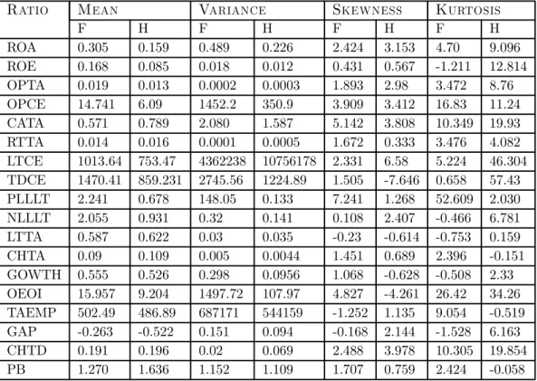
In Table 2 we present summary statistics for the ratios used.
Table 3 Summary Statistics
Ratio Mean Variance Skewness Kurtosis
F H F H F H F H ROA 0.305 0.159 0.489 0.226 2.424 3.153 4.70 9.096 ROE 0.168 0.085 0.018 0.012 0.431 0.567 -1.211 12.814 OPTA 0.019 0.013 0.0002 0.0003 1.893 2.98 3.472 8.76 OPCE 14.741 6.09 1452.2 350.9 3.909 3.412 16.83 11.24 CATA 0.571 0.789 2.080 1.587 5.142 3.808 10.349 19.93 RTTA 0.014 0.016 0.0001 0.0005 1.672 0.333 3.476 4.082 LTCE 1013.64 753.47 4362238 10756178 2.331 6.58 5.224 46.304 TDCE 1470.41 859.231 2745.56 1224.89 1.505 -7.646 0.658 57.43 PLLLT 2.241 0.678 148.05 0.133 7.241 1.268 52.609 2.030 NLLLT 2.055 0.931 0.32 0.141 0.108 2.407 -0.466 6.781 LTTA 0.587 0.622 0.03 0.035 -0.23 -0.614 -0.753 0.159 CHTA 0.09 0.109 0.005 0.0044 1.451 0.689 2.396 -0.151 GOWTH 0.555 0.526 0.298 0.0956 1.068 -0.628 -0.508 2.33 OEOI 15.957 9.204 1497.72 107.97 4.827 -4.261 26.42 34.26 TAEMP 502.49 486.89 687171 544159 -1.252 1.135 9.054 -0.519 GAP -0.263 -0.522 0.151 0.094 -0.168 2.144 -1.528 6.163 CHTD 0.191 0.196 0.02 0.069 2.488 3.978 10.305 19.854 PB 1.270 1.636 1.152 1.109 1.707 0.759 2.424 -0.058
At this point we will not comment on these statistics. We note however the need to use non-parametric tests to perform comparison of ratios. As the statistics reveal, often these ratios present strong leptokurtosis and skewness biases.
4 Statistical Methodology
The statistical methodology used is rather straight forward. It consisted of two separate tests:
1. We performed a non-parametric test of Wilcoxon, also known under the name of Mann & Withney U Test. This is one of the most robust and popular non-parametric tests on a two sample situation. The test allows us to seek the rejection of the hypothesis that the …nancial ratio in question are identical for the ”failed” and ”healthy” samples. This test was performed on all ratios of
interest in the eight categories. The standard practice in this type of situa-tions is to rank all observasitua-tions by value. Then, if the sum of the ranks of one sample di¤ers signi…cantly from that of the other sample, there exist a signif-icant di¤erence in the placement of both samples.17 In our case this means
that we combine, for each ratio, the values obtained for the two samples and rank them. The next step is then to verify whether the sum of ranks of the ”failed” sample and the ”healthy” sample equals the respective expected value or theoretical sum of ranks. This is the sum of ranks that would exist if both samples came from the same population. This is repeated for each …nancial ratio. The test statistic is aZ-test. For samples of our size the critical value for a 0.05 con…dence level is 1.96.
2. We estimated a Logit regression model on the sample of ”healthy” (0) and ”failed” (1) banks with the dichotomous variable as dependent variable and a reduced set of …nancial ratios as explanatory variables. This test, allows us to identify the subset of explanatory variables that explain best one or the other outcome with explicit consideration of interaction between variables. It also allows us to compute probabilities associated with an outcome for each member of the sample.
These are standard statistical procedures and, fto save space, we simply refer the reader to any statistics textbook for an exact speci…cation and more detailed description of the same.
5 Results
We present results in the same order that we presented the tests.
5.1 Wilcoxon Non-Parametric Test.
In Table 3 we present the results of the non-parametric rank test. The table is rather large, thus we have placed it at the end of the article. This table should be interpreted is as follows. Compare columns 2 (P) and 3 (P underH0). These
two columns represent the actual sum of ranks and the sum of ranks that should be found if the two samples came from the same population, respectively. When the hypothesis is rejected these columns should be approximately equal. This is so because the actual sum of ranks equals approximately the expected sum of ranks when the null hypothesis of no di¤erence holds. However, when columns 2 and 3 di¤er substantially for both samples (and when the di¤erence for one sample is important the same will happen to the other sample) then the interpretation is that the actual sum of ranks is not approximately equal to the expected sum of ranks under the null hypothesis. How di¤erent these sums of ranks are is measured by the computed
17The rank is considered to be preferable to the actual values for several reasons associated with
Z ¡statistic. This value is also function of the standard error of ranks. The last two columns are not strictly necessary but they provide the P ¡value associated to the statistic and the decision. In general a Z ¡statistic larger than 1.96 implies that there exist a statistically signi…cantly di¤erence between the two samples for the ratio in question with a signi…cance level of 0.05.
The results displayed in Table 3 are amazingly robust. In almost all categories/ratios the test suggests a di¤erence in values for ”failed” and ”healthy” banks in the ex-pected direction. Even for the category of charter value there is a ratio that passes the 0.1 con…dence level barrier. More speci…cally, for each category of ratio what this test implies is the following (see also Table 2 with general statistics):
² pro…tability, ”failed” banks are consistently more pro…table than ”healthy” banks across all ratios. In three out of four measures ”failed” are twice as pro…table than ”healthy” banks. This is perhaps a quite inexpected result. However it is perfectly consistent with a picture of ”failed” banks that operate in a much more aggresive manner;
² capital adequacy, ”failed” banks are consistently under-capitalized, however measured, when compared to ”healthy” ones. Clearly, banks with a better capitalization will be able to absorb with less di¢culties the macro shocks that are likely to occur during the FL process;
² quality of loan portfolio,”failed” banks start the FL process with a loan portfolio of less quality than ”healthy” ones. As with pro…tability the indicators are twice as large for ”failed” banks than for ”healthy” banks. This implies that the quality of the loan portfolio at the onset of the FL process is an important determinant of bank solvency;
² liquidity risk, ”failed” banks operate with lower liquidity ratios than ”healthy” ones;
² growth, if one accepts a con…dence limit of 0.1, then ”failed” banks display a higher growth rate than ”healthy” ones;
² e¢ciency,surprisingly ”failed” banks operate with higher e¢ciency than ”healthy” ones;
² interest rate risk, the interest rate risk exposure, as measured by the GAP of ”failed” banks is larger than that of ”healthy” banks. It is interesting to note that both samples display negative GAP measures, but that this negative Gap ratio is larger for the ”healthy” sample than for the ”failed” sample. On eof the possible interpretations of this result is that ”failed” banks hold a more important portion of their assets in the form of short-term interest-rate sensitive assets. In a context of FR this could be considered an aggresive strategie of asset management.
² charter value, as expected, ”failed” banks display a lower charter value than ”healthy” ones, implying that the former may be more prone to engage in moral hazard than the ”healthy” banks.18
The analysis of these ratios suggest that both types of ratios, those measuring loan porfolio quality and those re‡ecting management and risk-taking practices, are signi¢cantly di¤erent for the two samples, suggesting that they both play a role in determining the eventual solvency of the bank.
5.2 Logit Regression.
To execute the Logit regression we used a reduced number of …nancial ratios. The use of the complete set of 18 …nancial ratios would have yielded a too small number of degrees of freedom for a meaningful interpretation of results. Unfortunately, one set of ratios we were forced to eliminate was the ones measuring quality of loan portfolio (PLLLT and NLLLT). This limits the usefulness of the test.19 However, we can still
test whether management risk-taking practices, i.e. moral hazard, plays an important role in eventual insolvency. We present the ratios used in this ”complete model” and the values of the coe¢cients estimated via a maximum likelihood function in Table 4. We remind the reader that the dependent variable is the revealed state of the bank ”healthy” (0) and ”failed” (1).
18This particular test, in combination with the other ones, could be considered a test, albeit a
simple one, of the somewhat controversial theory that banks that display a higher charter value are more inclined to engage in risk enhancing moral hazard activities.
19We attempted nonetheless to run a model that would include these ratios. The purpose was to at
least an impression about the importance of the quality of the loan portfolio on failure probability. However, the number of usable observations dropped dramatically and the maximum likelihood procedure failed to converge even at very high number of iterations.
Table 4
Logit Regression
General Statistics
Log Likelihood -39.42
Cases Correct20 91 out of 108
Coefficients
Ratio Coe¢cient t¡statistics
Constant -1.454 -0.493 ROA -260.4 -1.888 ROE 21.40 2.139 OPTA 19.67 1.279 CATA 1.942 1.425 OPCE -3.722 -0.837 LTCE -0.037 -0.246 TDCE -0.044 -0.371 LTTA 3.486 0.955 CHTA 0.802 0.065 OEOI 0.066 1.839 GAP 3.761 2.041 CHTD -2.951 -0.648
The results of this regression reveals that bank failure is positively related to return on equity (ROE), operating e¢ciency (OEPO), interest rate risk (GAP), and negatively related to returns on asset (ROA). The number of correctly classi…ed observations is remarcably high. This result con…rms the observations made when interpreting the Wilcoxon test, that banks that operated more aggressively were the ones that fell in the category of ”failed” banks. A Logit regression that includes as regressors only the ratios that were signi…cant at the 0.10 con…dence level in the ”complete model” yields the following result:
¼ =¡1:416 + 15:199¤ROE+¡120:9¤ROA+ 0:06¤OEOI+ 2:42¤GAP
where¼ represents the probability of ”failing”. We call this the ”reduced model.” Using this reduced regression would have classi…ed correctly 98 out of 116 observa-tions!
The Logit regression also yields for each observation the probability of being correctly classi…ed (i.e. P(Yi = yi j Xi¯b, where yi is the actual value of Yi for
observation i). This give a measure of the quality of the prediction. We computed the means of these probabilities for the sample of ”failed” and ”healthy” banks. We present these values in Table 5.
20Cases correct is the number of observations for which the estimated probability of achieving
the observed value is greater than .5, and thus the ”predicted value” is the one which occurred. In this paper when we refer to correct classi…ed cases we mean for in-sample cases. The rather small number of observations available to carry out the study did not allow us to keep a subsample for out-of-sample tests of classi…cation correctness.
Table 5
Computed Probabilities of Correct Classi…cation (Mean of Samples)
Model ”Failed” ”Healthy”
Complete Model 0.44 0.75
Reduced Model 0.59 0.78
It is not surprising that it is easier to correctly classify ”healthy” banks than ”failed” ones given the superior number of observations available for the …rst sam-ple. Somewhat surprisingly is that the simple ”reduced model” performs better in predicting the outcome than the ”complete model.” A more in-depth analysis with additional information about bank accounts would most likely provide a richer ”re-duced model” with even larger predictive power than the one presented here.
6 Conclusion
In this paper presents a statistical analysis designed to distinguish, at the onset of a …nancial liberalization (FL) process those banks that are most likely to be at the origin of a banking crisis a few years later. The analysis is a response to the frequently observed fact that FL often are followed by banking crisis that may cost taxpayers enormous amount of resources in rescue operations. The study is based on a sample of 82 banks from Greece, Indonesia, Korea, Malaysia, Mexico, Thailand and Taiwan. The purpose of the work is to investigate two questions: 1) whether it is possible to statistically distinguish ”failed” banks (which we de…ne as those banks that may require taxpayers money support or may go bankrupt) from ”healthy” banks (de…ned as those banks that will perform well through the FL process). 2) assess to what extent the state of the loan portfolio and/or the management risk-taking practices (moral hazard) at the onset of the FL process, play a dominant role. For the …rst question, the results are surprisingly robust with most …nancial ratios used in the study displaying statistically di¤erent values for the sample of ”failed” and ”healthy” banks when using a non-parametric Wilcoxon test. Further a Logit model allows us to correctly classify 84% of in-sample observations. Given that the average delay from the moment of FL to bank insolvency is between four and …ve years, this means that it may be possible to identify with an anticipation of at least 4 years which banks may be the responsible of an eventual banking crisis!
For the second question, di¢culties in obtained the data limited our ability to test the alternative hypothesis. However, the evidences suggest that both, the state of the loan portfolio at the onset of FL and the risk-taking practices are important factors in in‡uencing the outcome. The tests allow us to state quite categorically that moral hazard does play an important role in determining bank insolvency. The di¤erences in ratios and the Logit regression suggest that banks that display a more conservative management and risk-taking practices are the ones that are more likely to eventually be revealed as ”healthy” banks. As a subsidiary result of this research we also shed some light on the interesting question of the e¤ect of charter value on the behavior of banks. Our data suggest that the banks that display a higher charter
value are those that engage in less risky bank management –i.e. less moral hazard– and are those that become classi…ed as ”healthy” banks.
References
[1] Joseph Aharony and Itzhak Swary. Additional evidence of the information-based contagion e¤ect of bank failures. Journal of Banking and Finance, 20:57–69, 1996.
[2] Edward I. Altman. Zeta analysis, a new model to identify bankruptcy risk of corporations. Journal of Banking and Finance, 1:589–609, June 1977.
[3] George J. Benston and Gerorge G. Kaufman. Is the banking and payment system fragile? In H. A. Benink, editor,Coping with Financial Fragility and Systemic Risk, pages 15–46. Kluwer Academic Publishers, Boston, 1995.
[4] Gerard Caprio and Daniela Kligebiel. Bank insolvency: Cross-country experi-ence. Washhington: World Bank, unpublished, 1996.
[5] Klaus P. Fischer Chavez, Jacqueline and Edgar C. Ortiz. Financial liberalization and bank solvency: A multicountry study. Research in International Business and Finance, 12, 1996.
[6] David C. Cole and Betty F. Slade. Indonesian …nancial development: A di¤erent sequencing? In Dimitri Vittas, editor, Financial Regulation: Changing the Rules of the Game, pages 121–162. EDI Development Studies, The World Bank, Washington, D.C., 1992.
[7] Douglas O. Cook. Determinants of bank stock returns and "too-big-to-fail". Working Paper, O¢ce of Thrift Supervision, February 1993.
[8] Hernan Cortes-Douglas. Financial reforms in chile: Lessons in regulation and deregulation. In Dimitri Vittas, editor, Financial Regulation: Changing the Rules of the Game. EDI Development Studies, World Bank, Washington, D.C., 1992.
[9] Asli Demirgüc-Kunt. Deposit- institution failure: A review of empirical litera-ture. Economic Review, FRB of Cleveland, 25:2–18, 4th Quarter 1989.
[10] Mathias Dewatripont and Jean Tirole. The Prudential Regulation of Banks, volume 1 ofThe Walras-Pareto Lectures. The MIT Press, Cambridge: England, 1994.
[11] Carlos Diaz-Alejandro. Good-bye …nancial repression, hello …nancial crash. Jour-nal of Development Economics, 19:xx–xx, 1985.
[12] Fabrice Dinh. Financial liberalization and banking crises in asian emerging mar-kets: Analysis of causality. Master’s thesis, Laval University, May 1996.
[13] Klaus P. Fischer, Jean-Pierre Gueyie, and Edgar Ortiz. Financial liberaliza-tion: Commercial bank blessing or curse? Journal of International Finance, 4, fortcoming 1996.
[14] Vicente Galbis. Liberalizacion del sector …nanciero bajo condiciones oligopolicas y la estructura de los holding bancarios. In Santiago Roca, editor,Estabilización y ajuste estructural en América Latina, pages 289–315. Escuela de Adminis-tración de Negocios (ESAN), Lima, Perú, 1985.
[15] Vicente Galbis. Sequencing of …nancial sector reforms. Technical Report WP/94/101, IMF, 1994.
[16] Heather D. Gibson and Euclid Tsakalotos. The scope and limits of …nancial liberalization in developing countries: A critical survey. Journal of Development Studies, 30:78–628, April 1994.
[17] Morris Goldstein and Philip Turner. Banking crises in emerging economies: Ori-gins and policy options. Technical Report 46, Bank of International Settlements, Monetary and Economic Department, Basle, October 1996.
[18] Jose F. Guzman. Liberalización, profundización …nanciera y los desafíos para la regulación y supervisión. In CEMLA, editor,Novena Asamblea de la Comisión de Organismos de Supervisión Y Fiscalización Bancaria de Améerica Latina Y el Caribe, pages 35–58, Mexico, D.F., 1993. CEMLA.
[19] Iftekhar Hasan and Jr. Gerald P. Dwyer. Bank runs in the free banking period.
Journal of Money Credit and Banking, 26:271–288, May 1994.
[20] Patrik Honohan. Financial system failures in developing countries: Diagnosis and prediction. Washington: Internationbal Monetary Fund, unpublished, 1996. [21] R. Barry Johnston. Sequencing …nancial reform. In Patrick Dowes and Reza Vaez-Zadeh, editors, The Evolving Role of Central Banks, chapter 20. Interna-tional Monetary Fund, Washington, D.C., 1991.
[22] R. Barry Johnston. The speed of …nancial sector reform: Risk and strategies. Technical Report PPAA/94/26, IMF, 1994.
[23] Graciela Kaminsky and Carmen Reinhart. The twin crises: The cause of banking and balance of payment problems. Board of Govrnors of the Federal Reserve System and the International Monetary Fund. Manuscript, 1995.
[24] Michael C. Keeley. Deposit insurance, risk and market power in banking. Amer-ican Economic Review, 80:1183–1200, 1990.
[25] William Lane, Stepehen Looney, and James W. Wansley. An application of the cox proportional hazard model to bank failure. Journal of Banking and Finance, 10:511–531, 1986.
[26] Catherine Mansell Carstens. De la represión …nanciera a las operaciones de mer-cado abierto. In CEMLA, editor,Reformas Y Reestructuración de Los Sistemas Financieros En Los Países de América Latina, pages 101–123. CEMLA, México, 1994.
[27] Alan J. Marcus. Deregulation and bank …nancial policy. Journal of Banking and Finance, 8:557–565, 1984.
[28] Daniel Martin. Early warning of bank failure: A logit regression approach.
Journal of Banking and Finance, 1:249–276, 1977.
[29] Ronald I. McKinnon. The Order of Economic Liberalization: Financial Control in the Transition to a Market Economy. The Johns Hopkins University Press, Baltimore and London, 1993.
[30] Maureen O’Hara and Wayne Shaw. Deposit insurance and wealth e¤ects: the value of being "too big to fail". Journal of Finance, 45:1587–1600, 1990. [31] Coleen C. Pantalone and Marjorie B. Platt. Predicting commercial bank failure
since deregulation. New England Economic Review, pages 37–47, July/August 1987.
[32] Sangkyun Park. Bank failure contagion in historical perspective. Journal of Monetary Economics, 28:271–286, 1991.
[33] Barron H. Putnam. Early warning systems and …nancial analysis in bank mon-itoring. Economic Review, 68:6–13, November 1983. FRB of Atlanta.
[34] Liliana Rojas-Suárez and Steven R. Weisbrod. Financial fragilities in latin américa: The 1980’s and the 1990’s. Occasional Papers 132, IMF, Washing-ton, D.C., 1995.
[35] V. Sundararajan. The role of prudential supervision and …nancial restructuring of banks during transitions to indirect instruments of monetary control. Journal of International Finance, 4, 1996. forthcomming.
[36] James B. Thomson. Modeling the bank regulator’s closure option: A two-step logit regression approach. Journal of Financial Services Research, 6:5–23, 1992. [37] Delano Villanueva and Abbas Mirakhor. Strategies for …nancial reforms. IMF
Table 3
Results of Wilcoxon Tests Ratio P(No. of Obs)21 PunderH
0 Std. Err. Comp. Z P-value Decision
F H F H Pro…tability ROA 4954 (51) 9074 (116) 4284 9744 287,789 2.326 0.02 Reject H0 ROE 5481 (53) 9397 (119) 4584 10293.5 301,538 2.972 0.003 Reject H0 OPTA 6122 (56) 10349 (125) 5096 11375 325,831 3.147 0.0016 Reject H0 OPCE 6184 (56) 10287 (121) 5096 11375 325,832 3.338 0.0008 Reject H0 Capital adequacy CATA 5096 (56) 11375 (125) 6527 9944 325,832 4.390 0.0001 Reject H0 RTTA 1716 (26) 7061 (106) 1729 7049 174,772 -0.069 0.945 Accept H0 LTCE 5986 (56) 10485 (125) 5096 11375 325,832 2.730 0.0063 Reject H0 TDCE 5818 (56) 9758 (120) 4956 10620 314,833 2.736 0.0069 Reject H0
Loan Portfolio Quality
PLLLT 2407 (42) 2153 (53) 2016 2544 133,444 2.930 0.003 Reject H0 NLLLT 601 (10) 65 (26) 481 185 28,311 -4.221 0.0001 Reject H0 Liquidity Risk LTTA 4691 (56) 11780 (125) 5096 11375 325,832 -1.241 0.214 Accept H0 CHTA 5096 (56) 11375 (125) 5866 10605 325,832 2.362 0.018 Reject H0 Growth GOWTH 4097 (48) 7228 (102) 3624 7701 248,209 1.903 0.056 E¢ciency OEOI 2893 (48) 7838 (98) 3528 7203 240,049 -2.643 0.008 Reject H0 TAEMP 1027 (20) 684 (38) 1121 590 61,124 1.529 0.126 Accept H0
Interest Rate Risk
GAP ratio 4007 (42) 7469 (109) 3192 8284 240,806 3.382 0.0009 Reject H0
Charter Value
CHTD 4654 (50) 9374 (117) 4200 9828 286,181 1.585 0.113 Accept H0 PB 698 (16) 5743 (97) 916 5529 121,424 -1.758 0.078 Accept H0
21We remind the reader that we took two years of observations for each bank, the one corresponding
to the FL event and the one for the previous year. Thus the numbers shown below correspond to the double of banks observed.
Appendix
Table A1 De…nition of Financial RatiosRatio Calculation
Pro…tability
Return on Assets (ROA) Earnings before taxesTotal Assets Return on Equity (ROE) Earnings before taxesEquity Operating Pro…ts of Assets (OPTA) Operating IncomeTotal Assets Operating Pro…ts of Equity (OPCE) Operating Pro…tsEquity
Capital adequacy
Capital over Assets (CATA) Total AssetsEquity Retained Earnings over Total Assets (RTTA) Retained EarningsTotal Assets Loans over Equity (LTCE) Total LoansEquity Deposits over Equity (TDCE) Total DepositsEquity
Loan Portfolio Quality
Reserves over Total Loans (PLLLT) Reserves Total Loans
Loan Losses over Total Loans (NLLLT) Loan Losses Total Loans
Liquidity Risk
Total Loans over Total Assets (LTTA) Total Loans Total Assets
Liquidity Ratio (CHTA) Liquid AssetsTotal Assets
Growth
Growth of Assets (GOWTH) Total Assetst¡Total Assetst¡1
Total Assetst¡1
E¢ciency
Operating E¢ciency (OEOI) Operating ExpensesOperating Income Total Assets over Employees (TAEMP) Total Assets
Number of Employees
Interest Rate Risk
GAP ratio (GAP) Rate Sensitive Assets¡Rate Sensitive Liabilities Total Assets
Charter Value
Liquid Assets over Deposits (CHTD) Total DepositsLiquid Assets Market over Book Value (PB) Market Value of EquityBook Value of Equity