Monetary Policy With Endogenous Firm
Entry
∗
Marwan Elkhoury
†Graduate Institute of International Studies, Geneva
Tommaso Mancini-Griffoli
‡Swiss National Bank, Paris School of Economics, and CEPREMAP First draft: March 2006. This draft: July, 2007
Abstract
This paper explores a new channel for the transmission of mone-tary policy through the extensive margin. In this paper, a shock to money induces firms to enter by affecting a measure of Tobin’s Q: the ratio of expected future profits to entry costs. In a dynamic stochastic general equilibrium setting, though, optimal consumption smoothing limits the flow of entering firms. As a result, the model generates pos-itively correlated, persistent and hump-shaped responses of output, consumption and firm entry to monetary shocks, as observed in the data. This is obtained via an endogenous source of inertia and despite minimal nominal rigidities, as only one-time entry costs – as opposed to goods prices or wages – are assumed to be sticky.
∗Thanks first and foremost to C´edric Tille for his guidance, insights and
encourage-ments. Sincere thanks also to Richard Baldwin, Florin Bilbiie, Hans Genberg, Fabio Ghironi, Jean Imbs, Michel Juillard, Bob King, Jean-Marc Natal, Scott Schuh and Tack Yun for extremely helpful comments. Thanks also to seminar participants at the Dynare conference in Paris (2006) and the Swiss National Bank (2007). We are indebted to Marc Melitz for inspiration and to have encouraged us to pursue the topic. All simulations were run usingDynarefor Matlab. The views in this paper are those of the authors and do not necessarily reflect those of the Swiss National Bank.
†[email protected]. 11A Avenue de la Paix, 1202 Gen`eve. Tel: +41 22 908 5959. ‡Corresponding author: [email protected]. Economics Research
Department, Swiss National Bank, B¨orsenstrasse 15, P.O.Box 2800, 8022 Zurich. Tel: +41 44 631 3631, Fax: +41 44 631 3911.
Keywords: monetary policy, firm entry, sunk entry costs, product variety, new keynesian models.
1
Introduction
Considerations of richer and more realistic firm dynamics are permeating fields as diverse as trade, real business cycles, open macro and recently mon-etary policy. Much of this impulse finds root in a burgeoning empirical liter-ature having turned the spot-light on firm entry as a key driver of observed macro-economic patterns. In response to these findings, theoretical models have emerged to link the entry decision of firms to product variety, aggre-gate productivity, export behavior, terms of trade, and markups, uncovering new propagation mechanisms and shedding light on thus far puzzling styl-ized facts. This paper follows the impetus provided by this growing body of literature and attempts to extend the reflection on firm dynamics to the field of monetary policy.
In particular, this paper’s innovation is to incorporate endogenous en-try into a monetary model and thereby emphasize a novel channel for the transmission of monetary policy. The appeal of this channel is it’s ability to reproduce stylized facts despite minimal exogenous sources of persistence. A temporary monetary shock, in this paper, generates persistent as well as hump-shaped responses of output, consumption, investment and new firm entry, as observed in the data. It also reproduces documented stylized facts showing the positive correlation of firm entry with monetary innovations. These results rest on an endogenous source of persistence and are found de-spite flexible goods prices. The only source of rigidity are stick sunk entry costs.
We construct a model based on monopolistic competition, in which firms have to pay a sunk cost to enter. These are meant to capture costs from the
set-up of operations, financing, hiring, R&D, marketing or other activities. For ease and clarity of exposition, we capture these sunk costs in a stylized fashion, by subsuming them into what we call legal fees, charged by lawyers. This is purely an artificial construct, or “trick”, to simplify the analysis. We also refer to firm entry throughout the paper, but the process is general enough to encompass the introduction of new products or the expansion of an existing firm or product into a new market.
We introduce nominal rigidities only in entry costs, or legal fees. We do so by assuming that lawyers set their fees according to a Calvo (1983) model. This allows monetary policy to be effective, despite goods prices remaining flexible throughout the analysis. A monetary shock affects a measure of Tobin’s Q, namely the ratio of a firm’s expected future profits to cost of entry, and propagates through the real economy by affecting investment in new firms, and thus consumption, output and other key variables. As a result, monetary policy is pro-cyclical with firm entry, as has been noted in the empirical papers reviewed below. This channel takes effect in addition to the more traditional interest rate channel of New Keynesian models.
The sluggish, hump-shaped responses central to our results rest on an endogenous source of persistence stemming from a tradeoff between con-sumption and investment, amplified by a time to build lag in production. We show that if lawyer fees are merely a transfer from firms to consumers, investment in new firms is not constrained by the impetus to smooth con-sumption. But if investment in new firms comes at the cost of consumption, a monetary shock will spread sluggishly through the economy.
impact of monetary policy stemming from variations in product variety. We do so by showing that the expansionary effects of a monetary shock (mea-sured in welfare-relevant terms) depend on consumers’ love of variety. This approach is inspired by the seminal work on estimating the gains from variety expansion by Broda and Weinstein (2004, 2006).
Evidence linking monetary policy to firm entry is starting to trickle through the literature. Ghironi and Melitz (2005), as well as Bilbiie et al. (2005) document in detail the notable pro-cyclicality of firm entry. The difficulty is to extract from these results the correlation between monetary policy and firm entry: it could be positive when growth in GDP emanates from an expansionary monetary policy surprise, but negative when central banks tighten policy to cool a period of strong output growth. Bergin and Corsetti (2005) help untangle the two effects using a VAR methodology. They conclude that monetary expansions are positively correlated to firm entry. These findings are corroborated in Lewis (2006) who, in a similar VAR ex-ercise, identifies both monetary and real shocks and captures the positive and hump-shaped response of firm entry to a monetary surprise. Davis et al. (1998), in their influential book Job Creation and Destruction, find sim-ilar results, but at a relatively lower frequency, tied to trends in monetary policy. These findings substantiate common intuition that monetary policy affects firm behavior directly, not only through consumer demand, especially if entry is taken generally to encompass capacity expansion, new product introductions, project developments in addition to new firm incorporations.
There also exists mounting, if not comfortably established, evidence for the persistent as well as hump-shaped responses of consumption, output and
investment that our model generate. Most recently, Christiano et al. (2005) revisit some of their seminal 1999 results using a limited information VAR procedure to highlight that an expansionary monetary policy shock induces “a shaped response of output, consumption and investment, a hump-shaped response in inflation, a fall in the interest rate, a rise in profits, real wages and labor productivity, and an immediate rise in the growth rate of money” (Christiano et al., 2005, p. 6). In an influential study, Romer and Romer (2004) corroborate these results after pinpointing monetary policy surprises thanks to the meticulous exercise of accounting for the intentions, information and forecasts discussed in FOMC meetings. Their implied re-sponse of output to a monetary shock follows a hump-shaped pattern, with, interestingly, an initial much smaller hump in the opposite direction. The impulse response functions emanating from our model exhibit these same features, sharing, in some cases, Romer and Romer’s ‘dual hump’ pattern.
The predictions in this paper also resonate with a well established liter-ature outside the field of monetary policy – that of sunk costs and market structure in the field of IO. As mentioned earlier, the transmission channel for monetary policy at the heart of this paper goes from a monetary shock to sunk costs to firm entry. The latter part of this causal link is a central theme in the IO literature, captured with great clarity and detail in Sutton’s (1991) influential book Sunk Costs and Market Structure. The book builds a theory by which concentration, or the number of firms in a given industry, is a positive function of market size and a negative function of set-up, or sunk, costs. This relationship is so general, argues Sutton, that it fits both industries where goods are homogeneous and horizontally differentiated (as
in Shaked and Sutton, 1987) and is supported by a very comprehensive set of case studies.
This paper contributes to several literatures, in part by virtue of strad-dling the traditional New Keynesian literature and that on firm entry dynam-ics. With respect to the former, we build the monetary side of the model using a dynamic stochastic general equilibrium framework, as prescribed by much of the literature’s representative works, such as Goodfriend and King (1998), Clarida et al. (1999), Gali (2002), or Woodford (2003). We add money in the utility function and budget constraint, yet we introduce a much less severe form of price stickiness than inherent in these models, by allowing goods prices to remain flexible throughout the analysis. We only restrict the one-time sunk entry costs from adapting immediately to monetary surprises by imposing a time-contingent Calvo (1983) pricing behavior on lawyers. Despite this minimal source of rigidity, monetary policy has significant real consequences.
One of the drawbacks of standard New Keynesian models is their inability to generate sufficient sluggishness (slow to move away from steady state) and persistence (slow to move back to steady state) in the responses of inflation and real variables to a monetary shock. Gali and Gertler (1999), as well as Gali (2002), discuss this limitation and offer an inroad to a solution, by assuming that a certain percentage of firms are backward, and not forward, looking. Although this assumption alters the results as desired, this line of reasoning has been criticized as somewhat ad-hoc.
More recent models have noticeably improved predictive capacity while offering sounder micro-foundations, but at the cost of a series of exogenous
as-sumptions introducing rigidities; a direction we try to avoid. One of the most successful papers in capturing hump-shaped responses to monetary shocks is Christiano et al. (2005).1 This model essentially dampens the reaction of marginal costs to monetary shocks, by introducing wage stickiness and variable capital utilization, as well as habit formation in preferences and adjustment costs in investment. We hope to provide an alternative model-ing approach, restmodel-ing on fewer sources of exogenous inertia and emphasizmodel-ing closer ties with microfoundations.
With respect to the literature on firm entry dynamics, this paper’s in-novation is to extend the techniques and reflections to the field of monetary policy. The backbone of our model is inspired in great part from the in-fluential work of Bilbiie et al. (2005) in the real business cycle literature. Indeed, we borrow this model’s firm dynamics based on sunk entry costs and a one period lag separating entry from production, thus making the number of firms a state variable. In fact, it is these two elements that differentiate the real part of our model from the earlier work of Chatterjee and Cooper (1993) who also consider endogenous entry but with fixed period-by-period costs and instantaneous entry. Like in Bilbiie et al. (2005), we also allow con-sumers to invest in new firms as an additional channel to bring wealth from one period to the next. Despite these similarities (which we try to emphasize for ease of reading by adopting similar notation wherever possible), we differ not only in adding a monetary side to the model, but also in our specification of entry costs as being only in consumption units, and not absorbing labor from production.
1Other seminal, but older papers, are Fuhrer and Moore (1995) or Blanchard and Katz
Some other papers have recently tackled the impact of monetary policy on the extensive margin, each with a different perspective and each – like ours – tentatively suggesting an inroad into this new literature. While our paper concentrates on the propagation mechanism of monetary policy and obtaining realistic impulse response functions, Bergin and Corsetti (2005) focus instead on the welfare implications of monetary policy. Indeed, Bergin and Corsetti (2005) simplify firm dynamics to concentrate instead on a rich discussion and comparison of optimal policy rules, as well as build an argument for the role of central banks to regulate product variety. Firms, in their paper, only live two periods and goods prices are set one period in advance. This yields a positive correlation between a monetary expansion and firm entry, as well as some persistence in entry, but no persistence in output, nor, by extension, consumption. More recently, Lewis (2006) and Bilbiie et al. (2007) offer similar perspectives on the issue. Lewis (2006) closely reproduces the RBC model in Bilbiie et al. (2005), but adds monopoly power in wage setting, thereby making monetary policy effective. The model is especially oriented to inform a convincing empirical part in which a VAR methodology is used to estimate impulse responses to both real and monetary shocks. Finally, Bilbiie et al. (2007) construct a model with sticky goods prices yielding a somewhat roundabout but innovative transmission channel of monetary policy going from interest rates to bond prices, to equity prices, to marginal costs, to inflation. The model allows for a rich discussion of optimal policy and comparisons to traditional New Keynesian models. It also produces desirable predictions of pro-cyclical profits and output, yet produces anti-cyclical entry. The latter comes from the distortionary effects of inflation on
entry, as firm profits are affected by quadratic price adjustment costs.2 Finally, it is important to distinguish this paper from the New Keyne-sian monetary literature with endogenous, or firm specific, capital and time to build lags. It is true, as Bilbiie et al. (2005) point out, that there is a parallel between the number of firms and capital stock, as well as between firm entry and investment. Yet, especially in monetary models, the paral-lel is limited. In models such as Woodford (2005), Mash (2002), Casares (2002), or even Christiano et al. (2005), a long time to build lag as well as sticky prices, sticky wages and adjustment costs are necessary to yield plau-sible results, contrarily to our reliance on endogenous sources of persistence. In particular, the substantial time to build lag is an integral and external source of sluggishness in these models, while in our model the one period lag exists primarily for technical reasons: to generate a difference equation. Sluggishness is instead rooted in consumption smoothing.
This paper is organized as follows. Section (2) lays out the benchmark model under flexible entry costs and section (3) overviews the correspond-ing impulse response functions emanatcorrespond-ing from a shock to entry costs. Go-ing through this initial exercise achieves three goals. First, it presents the model’s core elements, which are common to the sticky entry cost
formu-2Other papers of particular interest, but more distantly related, are worth mentioning.
Stebunovs (2006) considers the impact on bank deregulation on entry, emphasizing the role of sunk entry costs. Ghironi and Melitz (2005) is the primary paper reviving interest in firm dynamics in an open macro framework, suggesting an endogenous explanation for the Harrod-Balassa-Samuelson effect and a new hypothesis for the terms of trade effect of a productivity shock. Corsetti et al. (2005) draw an important distinction between productivity gains that lower marginal costs versus entry costs and study the effect of each on terms of trade and welfare. Finally, Chen et al. (2006) show how greater openness increases average productivity and decreases markups, thus keeping inflation in check. Each paper incorporates different aspects of firm dynamics to reach novel conclusions and insist on the interplay between microfoundations and macro phenomena.
lation. Second, it introduces the endogenous source of inertia in a simple environment. Third, it builds intuition for the transmission of monetary pol-icy, since a monetary shock affects the economy in similar ways as a shock to entry costs. Section (4) formally introduces nominal rigidities in entry costs and shows how monetary policy can be effective. Section (5) follows with a discussion of simulation results under sticky entry costs. Finally, section (6) concludes.
2
The benchmark model with flexible prices
and entry costs
2.1
Firms’ basics
Firms are assumed to be homogeneous. Given symmetry, we avoid using the i subscript to denote firm specific variables and instead use lower case letters unless otherwise noted (by contrast, capital letters capture aggregate variables). Firms employ only labor, lt, and produce with a common level of
productivity, Zt. Output per firm can be summarized as:
yt=Ztlt (1)
Firms choose an optimal price to maximize profits given by: dnt = pt− Wt Zt yt (2)
where Wt is the nominal wage, and the superscriptn indicates nominal
vari-ables, wherever a distinction is called for. As is usual in a CES environment (specified later), the resulting optimal price corresponds to a fixed markup over nominal marginal costs:
pt= θ θ−1 Wt Zt (3)
where θ > 1 is the degree of substitution between varieties in the CES con-sumption index (defined later).
2.2
Firm dynamics
Firms are not only free to set their price, but also to enter the economy, a decision they make if their expected profits pay back a sunk entry cost, fE,t. Contrarily to Bilbiie et al. (2005), we define entry costs not in terms of
effective labor units, but of consumption units, again with the goal of intro-ducing the minimal set of assumptions necessary to obtain realistic impulse response functions. We will see later how this cost is pivotal to introduce nominal rigidities, as it can be seen as sticky or determined in advance.
There are many possible interpretations for such an entry barrier. These include costs such as setup, recruitment, market research, financing, product adaption, advertising, R&D, or legal. For simplicity and clarity of exposition, we subsume all possible costs into the latter and assume that firms must pay a lawyer an amount fE,t before entering. Technically, this is equivalent to
assuming a horizontal supply curve for legal services at the level fE,t. Again,
as highlighted in the introduction, this is purely an artificial construct to simplify the analysis; when speaking of lawyers, we should in fact continue to keep in mind the above mentioned sources of entry costs.
Firms weigh these entrance fees against the expected net present value of profits from engaging in business. In doing so, firms also take into account an exogenously defined probability δ of being hit by a so-called “death shock”,
inducing them to exit.3 Thus, firm value is defined as: vt = Et " ∞ X s=t+1 [β(1−δ)]s−t Cs Ct −γ ds # (4) where β is a subjective time discount factor and the consumption ratio ap-pears as a stochastic discount factor to take into account variations in output from one period to another.
We know that at equilibrium, when all firms have entered, the expected net present value of profits must equal the entry cost. Indeed, when these two measures are equalized, there is no more incentive for additional firms to enter. Thus, we call this point the free entry condition, defined as:
vt=fE,t (5)
The last piece to the puzzle is the time to build lag which we assume characterizes entering firms, as in Bilbiie et al. (2005). Mathematically, this is an important assumption to giveNt, the state variable, a proper equation of
motion. From an intuitive standpoint, the assumption is just as defendable, as new firms may have to build clientele, a distribution network, a brand or simply a new product, after sinking their entry costs, but before being able to sell anything. The equation of motion for the number of firms is therefore Nt= (1−δ)(Nt−1+NE,t−1) (6)
whereNE,t−1 is the number of firms that entered in periodt−1 and are able to produce in period t. Thus, Nt is the number of active firms in any given
period t.
3This is a simplified, yet important assumption to keep the number of firms finite and
ensure that the number of firms returns to equilibrium after a shock. A more elaborate form of this assumption could account for state- or time-contingent exit, as in Hopenhayn (1992a, 1992b). See Melitz (2003) for a more detailed discussion of both entry costs and exit shocks.
2.3
Introducing the consumption-investment tradeoff
Before considering the equations characteristic of consumer demand, it is important to discuss a fundamental assumption giving rise to the inertial responses of the model’s real variables. Consumers are worker-owners. Their revenues, made up of wages and firm profits, account for aggregate pro-duction. From these proceeds, they decide how much to consume and how much to invest in new firms by financing entry costs. In turn, new firms pay these sunk costs to a representative lawyers who, we assume, consumes the totality of her earnings. So from an aggregate standpoint, equilibrium is maintained and total consumption (from consumers and lawyers) equals output. But from the standpoint of consumers, there arises an important tradeoff between consumption and investment. Although investment is at-tractive to create firms which later pay dividends, it comes at the cost of foregoing present consumption. Thus, the impetus to smooth consumption bestows noticeable persistence to investment. In appendix A.1 we show how consumers’ and lawyers’ consumption can be aggregated such that the usual CES results hold.
In the appendix (A.4 – A.7), we also introduce a second variant of the baseline model considered here, in which there is no tradeoff between sumption and investment, since lawyers simply rebate their earnings to con-sumers without absorbing any of the economy’s production. This is a stan-dard assumption, characteristic, for instance, of models with endogenous capital. Thus, consumption is not constrained by the creation of new firms. It is useful to juxtapose these two variants, as we do when discussing re-sults, to help emphasize the key role played by the consumption-investment
tradeoff.
2.4
Consumer behavior
In this section and those following, we consider only the consumption of con-sumers, while we postpone the analysis of the consumption of lawyers (whose utility function is isomorphic, except that they have an infinite discount fac-tor and thus undertake no investment; details are provided in appendix A.1). We come back to join the two sources of consumption when considering ag-gregate accounting in section 2.7.
The model is characterized by a representative consumer maximizing her infinite lifetime utility over consumption, Ct, real money balances, Mt/Pt
and leisure, Lt. For simplicity, we assume a separable utility function given
by: Ut= Et " ∞ X s=t βs−t C 1−γ s 1−γ + (Ms/Ps)1−ν 1−ν − L(sϕ+1)/ϕ (ϕ+ 1)/ϕ !# (7) where β is a subjective discount factor.
The budget constraint must be altered slightly with respect to standard monetary models to account for firm dynamics, by allowing consumers to invest in risk free bonds as well as in a risky but potentially more rewarding mutual fund of firms. Each period, consumers can choose to buy a share xt
of this fund, at a price equal to the expected net present value of profits of all existing firms: vt(Nt+NE,t). Investment in the mutual fund yields dividends
one period later, equal to profits of all operating firms, Nt+1dt+1, in addition to the liquidation value of the portfolio, vt+1Nt+1. Thus, the representative consumer faces the following constraint, written in nominal terms (where,
again, the superscript n clarifies, if necessary, when a variable is nominal): PtCt+Mt+R−t1Bt+vtn(Nt+NE,t)xt=
Mt−1+Bt−1+WtLt+ (dnt +v n
t)Ntxt−1+Tt (8)
where Rt ≡ (1 +it) and it is the nominal interest rate, Bt are zero coupon
nominal bonds, and Tt are lump sum seignorage transfers, such that Mt =
Mt−1+Ttin equilibrium. Note that by making use of the free entry condition
(5), the amount consumers allocate to financing new firm entry, vtnNE,txt, is
in fact the sum of all entry fees paid to lawyers, fn
E,tNE,txt. As per the
earlier discussion on the consumption-investment tradeoff, these fees are re-linquished to lawyers and thus do not show up on the right hand side of the budget constraint (as they would if they were rebated to consumers, as in the model’s second variant presented in the appendix).
Aggregate consumption,Ct, is defined as:
Ct=At Z Nt c(tθ−1)/θdi θ/(θ−1) (9) whereAt ≡N ξ− 1 θ−1
t , as in Benassy (1996).4 This term allows us to dissociate
consumers’ love of variety from the elasticity of substitution between goods. This is particularly important in our case since we work with variables that are “welfare relevant” in the way that they take into account the effect of variety on consumer utility. Thus, the use of At allows us to explicitly test
the robustness of our results to the link between variety and utility. Indeed, we may either be interested in measuring welfare, or in matching commonly available data (since most statistical agencies do not account for variety in
4It is becoming increasingly common to find such a specification in the literature. See,
for instance, Corsetti et al. (2005), Bergin and Corsetti (2005), or the appendix of Bilbiie et al. (2005).
reporting prices, or at least do so at a low frequency). Indeed, note that when ξ = 1/(θ−1), the above consumption index simplifies to the classic Dixit-Stiglitz (1977) case, but when ξ = 0, there is no more love of variety and, in particular, aggregate prices equal firm specific prices, as is evident from the definitions below.
Accordingly, aggregate prices are found by summing firm specific prices in the following way:
Pt= 1 At Z Nt pt(i)1−θdi 1/(1−θ) (10)
so that the relative price, ρt can be expresses as:
ρt≡pt/Pt=Ntξ = [θ/(θ−1)]ωt/Zt (11)
since pt is the same for all firms. The relative price ρt will lead to useful
simplifications down the line. For now, it is important to emphasize that when ξ is positive, a rise in the number of firms will depress the aggregate price Pt, everything else equal. This is commonly referred to as the variety
effect. More firms offer a wider range of choices to consumers, thus increasing value per unit of expenditure. In this way, the aggregate price is “welfare relevant” (as are all real variables in our model), capturing “subjective value” as perceived by consumers.
2.5
Optimality conditions
On this backdrop, consumers optimize both between consumption, leisure and real money held in any given period, as well as between consumption in subsequent periods. This yields the following first order conditions:
With respect to real money balances: Mt Pt ν = C γ t 1−R−t1 (12)
With respect to labor (the labor supply function): Wt
Pt
=L1t/ϕCtγ (13)
With respect to bonds (the Euler equation in bonds): Ct−γ =βRtEt Ct−+1γ Pt Pt+1 (14) With respect to shares (the Euler equation in shares):5
Ct−γ =β(1−δ)Et dt+1+vt+1 vt Ct−+1γ (15) Total demand for any given variety in periodt is instead given by:
yt=Aθt−1 pt Pt −θ Yt (16)
where Yt represents total expenditure on goods, equal to both consumers’
and lawyers’ consumption, as shown in section 2.7 below and discussed in more details in appendix A.1.
2.6
A closer look at the labor market
The aggregate pricing condition (11) and the optimal firm price equation (3) can be combined to yield an expression for the real wage ωt:
ωt =Zt
θ−1 θ N
ξ
t (17)
which is in itself an interesting equation, underlying the fact that as the number of firms increases, real wages must also increase to attract more
5Note, as is standard, that the forward solution to this Euler equation yields the
workers as needed by the greater number of firms. The above expression, along with the labor supply function (13), yields an expression for total labor employed as a function of the number of firms and consumption:
Lt =Ntξϕ θ−1 θ ϕ ZtϕCt−γϕ (18)
where it is clear that labor supply rises in tandem with real wages, but decreases with consumption, due to the decreasing marginal utility of con-sumption.
We also know that in aggregate, by assuming full employment, labor market accounting suggests that Lt = Ntlt.6 We then specify an aggregate
production function taking the form Yt = Ntρtyt = Ntξ+1yt, since all firms
are homogeneous and where ρt is included to convert output in terms of the
consumption good (in real terms). Coupled with the firm level production function (1), this allows us to obtain an interesting form of the aggregate production function: Yt=N ξ tZtLt=N ξ(1+ϕ) t Z 1+ϕ t θ−1 θ ϕ Ct−γϕ (19)
where the number of firms enters to capture the impact of variety on output, again underscoring the “welfare-relevant” nature of our real variables. This effect is in fact both direct and indirect, as shown by the inclusion of Nt
in the middle equation as well as in the far right equation, where it enters through real wages and labor supply.
6Note that this labor market accounting condition is different from the more
compli-cated equivalent found in the New Keynesian literature, as in Gali (2002), where, due to Calvo pricing, not all firms charge the same price at any given time, thus producing different amounts of output and employing different numbers of workers. In that case, we cannot simplify the integral Lt=RN
tltdi toLt=Ntlt, as above, but must take into
Finally, using the equation for profits (2), the equation for relative prices (11), the labor supply equation (18) and the aggregate production function above (19), we derive a useful expression for firm profits:
dt=
Yt
θNt
(20) Thus, firms’ profits naturally increase with aggregate output and decrease with the degree of substitutability between goods (a measure of competitive intensity) and the number of firms (which, as per the variety effect discussed earlier, increase each firm’s relative price ρt, thus depressing sales per firm).
This latter effect, though, is partially offset by the positive relationship be-tween output, Yt, and the number of firms.
2.7
Aggregate accounting
When aggregating the budget constraint over all consumers, and imposing equilibrium conditions such that bonds are in zero net supply (orBt=Bt−1 = 0), the representative consumer holds the entire equity portfolio (or xt =
xt−1 = 1) and lump sum transfers from seignorage exactly match money growth (or Mt=Mt−1+Tt), we obtain:
PtCt+vtnNE,t =WtLt+dntNt =Ytn (21)
where the left hand side represents aggregate consumption and net ment, and the right hand side labor and profit revenue (or returns on invest-ment) which can be shown to equal aggregate output (see appendix A.1 for the derivation), thus satisfying general equilibrium.
2.8
Steady state analysis
The complete derivation of steady state results appears in appendix A.2. Here, we instead report the results central to our story, namely the correlation between entry costs and consumption as well as the number of firms. The two equations we retain from the appendix are:
N = 1−δ δ Z (1+ϕ) θ−1 θ ϕ Nξ(1+ϕ)C−γϕ−C /fE (22) and C =fEN θ 1−β(1−δ) β(1−δ) − δ (1−δ)θ (23) These equations are especially eloquent (after some manipulation, as show in appendix A.2) on the long term negative effects of a rise in entry costs on the number of firms and consumption. Indeed, as shown in appendix A.2, ∂f∂N
E < 0, confirming general intuition. An increase in fE raises firm value as confirmed by the free entry condition (5). Recall that firm value, v, is also equal to the expected net present value of profits. Thus, for a constant discount factor, the only way that v can appreciate is for profits to increase as well. And as discussed above, profits grow as the number of firms diminishes and output per firm rises. Thus, not only does the steady state analysis confirm the intimate relationship between the entry cost and the number of firms, as intuition would have told us from the beginning, but it turns the spotlight on the free entry condition as the main constraint on firm dynamics. To complete our overview of the steady state, we also note that ∂f∂C
E > 0 (also shown in the appendix), since fewer firms will need less investment to offset dying firms and thus allow for more consumption.
2.9
Solving for the model’s dynamics
Our goal here is to define a system of minimal dimensions sufficient to solve for the model’s state variables. The Euler equation in shares (15) constitutes the first difference equation in Ct and Nt. The second equation comes from
the equation of motion of firms (6). In both cases, we must first solve for the number of new firms, NE,t.
To do so, we use the aggregate accounting condition (21), which acts as a constraint on how much investment can be undertaken given a level of consumption and earnings. We obtain:
NE,t =
Zt1+ϕ θ−θ1ϕNtξ(1+ϕ)Ct−γϕ−Ct
fE,t
(24)
Appropriately, in steady state, ∂NE/∂fE < 0, as well as ∂NE/∂C < 0,
as shown in appendix A.2. This indicates that as entry costs increase fewer firms are created, thereby confirming that there is indeed a tradeoff between investing in new firms and consuming. The solution to NE,t can then be
plugged into the equation of motion of firms which, with the Euler equation in shares, yields a system of two difference equations with a stable solution. Appendix A.3 presents this system in linearized form, as well as the additional equations needed to find the remaining variables of interest, once the paths for Ct and Nt have been resolved.
3
Simulation results under flexible prices and
exogenous entry costs
3.1
Calibrations
In order for our results to be comparable to those in the relevant literatures, we employ standard parameter values to calibrate our model. We assume log utility for consumption and thus set γ = 1, in line with real business cycle models, such that wealth and substitution effects cancel and the model be consistent with a balanced growth path. We follow Gali (2002) who draws from Chari et al. (1997) in setting the semi-elasticity of money demand,ν, to unity. We also work with a very low wage elasticity of labor supply since we consider a short run impact, and thus setϕ= 0.25. We relax this assumption in the more detailed analysis of sticky entry costs dynamics. As is standard in the real business cycle literature, we interpret periods as quarters and set β = 0.99. We then follow Bilbiie et al. (2005), who set the elasticity of substitution between goods, θ, to 3.8, as in Bernard et al. (2003), instead of the higher 6 used by Rotemberg and Woodford (1992) or 11 as in Gali (2002). We also set the death shock as in Bilbiie et al. (2005) to 0.025 in line with findings of approximately 10% labor destruction per year. In addition, we work with ξ= 1/(θ−1) as in the standard Dixit-Stiglitz (1977) case, so that the love of variety and the elasticity of substitution between goods concur. We introduce different values of ξ in later robustness tests. Finally, for all simulations in this paper, we consider that productivity remains constant.
3.2
Benchmark model with tradeoff
In these simulations, we concentrate on shocks to entry costs, to build in-tuition for the more complex mechanisms underlying the transmission of monetary policy. In figure 1, we therefore limit our attention to the variables most instructive for our model’s fundamental dynamics: Ct, Nt, and NE,t.
We consider the shock to entry costs to be temporary. We thus assume
b
fE,t+1 =φfbE,t+t, wheretis increased by 1% at the time of the shock. This
yields a path of sunk costs shown in figure 1, returning to steady state after 50 periods. But the duration of the shock is an artifact of our particular parameter values, notably of our somewhat arbitrary choice ofφ = 0.9. It is rather the shock’s effect on other variables that is central.
The first result to stand out is the persistence of the model’s variables over and above that of entry costs. This can be seen most clearly in the impulse response of the number of firms which strays from steady state for about 70 periods (thus 40% longer than entry costs). In graphs generated with φ= 0.09, this result is even more striking; entry costs are back at their steady state level within a few periods, but the number of firms only returns to steady state after about 35 periods.7
The tradeoff between consumption and investment – at the origin of the inertia noted above – is most evident in the path of consumption. Initially, when entry costs are lowest and investment (NE,t) at its peak, consumption
must decrease below steady state to satisfy the budget constraint. Only after a few periods does consumption rise again, following the increase in the number of firms.
Investment – or the creation of new firms – peaks early, and later over-shoots its steady state. This illustrates several mechanisms. First, there are intertemporal effects, in that firms try to enter as close as possible to the trough in entry costs. This explains the drop to below steady state invest-ment after the original peak. But, second, because of the impetus to smooth consumption, investment is not instantaneous, but stretches over the first 25 periods. As a result, the number of firms and consumption follow a regu-lar hump-shaped pattern. This result has potentially important empirical implications, suggesting that the contemporaneous correlation between en-try costs and the number of new firms would be not be as high as perhaps intuitively expected, even if, in fact, the two are intimately related.
Finally, our results substantiate our discussion of the steady state. In-deed, the number of firms moves in the opposite direction as entry costs. As discussed earlier, lower sunk costs depress expected firm value in equlibrium, calling for lower profits and thus a greater number of total firms.
3.3
Benchmark model without tradeoff
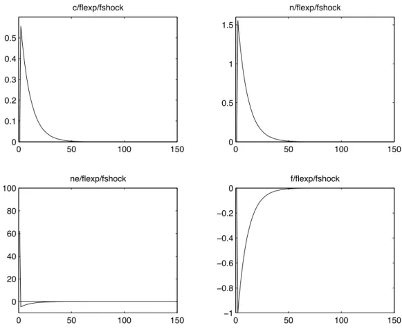
As mentioned earlier, we develop a second variant of the benchmark model (in appendix A.4 – A.7) where the fees received by lawyers are rebated to consumers, thus nullifying the tradeoff between consumption and investment. The impulse responses in this second variant are worth briefly dwelling upon, as they clearly show the central role played by the consumption-investment tradeoff in generating persistence and sluggishness. Indeed, a look at figure 2 immediately confirms that any inertia in the number of firms or consumption only mimics that of entry costs. In other words, there is no additional inertia in the system than that exogenously assumed in the driving variable.
The behavior of investment – or the number of new firms – is interesting none-the-less. With respect to the earlier variant, there is a much stronger inter-temporal shift in the creation of firms towards the period immediately following the shock. Indeed, that is when sunk costs are lowest. Although they remain below steady state for another fifty periods, firms prefer to take advantage of the most favorable possible conditions for entry, especially when investment is not constrained by consumption smoothing objectives. As shown in the graph, firm creation even becomes negative after the initial boom. We therefore notice no smoothing of investment what-so-ever (as a result of the lack of tradeoff with consumption).
Consumption (equal to output in this variant of the model since lawyers don’t consume; see appendix A.5 for details) instead follows the number of producing firms. This confirms our earlier discussion suggesting that although firm-specific output decreases with more firms, aggregate output increases. Finally, the fact that consumption is free to increase while new firms are created comes from the lack of tradeoff between consumption and investment.
4
The model with nominal rigidities
4.1
The channel of transmission
We have seen that firms decide to enter based on the relationship between expected profits and cost of entry. Thus, in order to be effective, monetary policy must be in a position to alter either one, or the ratio of the two, which is akin to Tobin’s Q. Of course, from a modeling standpoint, this poses an interesting question. On which side should nominal rigidities be modeled:
expected profits or costs of entry? Expected profits are discounted by the real interest rate, as seen in equation (4).8 A possible channel for monetary policy transmission would therefore be to affect the real interest rate, and thereby the net present value of firm profits and in turn firm entry. Although plausible, we choose to emphasize the reverse of the coin, namely the effect of monetary policy on the cost of entry. We do so for four major reasons which we enumerate below. Nonetheless, we should not loose sight of the fact that fundamentally, in our model, monetary policy affects Tobin’s Q, and through that, investment and consumption.
First, we aim to introduce minimal exogenous persistence in order not to steal the spotlight from the model’s endogenous source of inertia discussed at length above. The link between monetary policy and real interest rates typically comes by assuming price rigidity in the goods market. But in our case, this would introduce an additional source of persistence that would be hard to untangle in the interpretation of results. Second, assuming that monetary policy affects the real interest rate could also come from a rigidity in nominal rates. But this would entail modeling at least a rudimentary credit market and possibly allowing firms to finance entry costs by issuing risky corporate debt; a very plausible assumption, yet one that detracts from the model’s simplicity.9 Third, expected profits are generally hard to estimate and usually expressed with a wide range. Changes in real interest rates do little to change these vague forecasts. Instead, what is more tangible to firm
8Where, as per the Euler equation in bonds (14), the stochastic discount factor
βCs Ct
s−t
is equivalent to the real interest rate, defined as Rt−(Pt+1−Pt) in linear
terms.
9The work of Stebunovs (2006), mentioned in the introduction, could be used as a basis
managers and entrepreneurs is the cost of entry. Changes in these are an important driver of investment decisions.10 Fourth, we like to emphasize the central role played by entry costs, in order to pick up where the IO literature leaves off, namely in linking firm entry, or concentration, to a market’s sunk entry costs. Shaked and Sutton (1987) and Sutton (1991), for instance, make this relationship the center piece of their analysis.
4.2
Introducing nominal rigidities in entry costs
Given the above arguments, we introduce stickiness in entry costs, or lawyer fees. This allows a monetary surprise to affect the real value of entry costs and thereby engender similar reactions in the model’s variables as seen in our earlier exercise under flexible prices and exogenous entry costs. More specifically, we assume that lawyers set their fees as in the model of Calvo (1983). Following the usual modeling route would have led us to working with imperfectly differentiated lawyers. Yet, in our case, this would have complicated the analysis and detracted from the plausibility of the story: why should lawyers be differentiated? Where do they derive monopoly power? Where do profits go to? To circumvent these issues, we instead assume a representative lawyer (of a pool of perfectly competitive lawyers), who faces a probability of not being able to reset her price in any period.11 In the end, results for the optimal setting of fees are equivalent, in linear form, to a more standard imperfect competition Calvo model.
We thus work with a representative lawyer able to reset her price each
10This resonates with anecdotal evidence related by entrepreneurs and venture
capital-ists that ideas abound, but the main limitation to their development is the availability or cost of funding.
period with a probability (1−λ). Recall that total expenditures on entry fees are given by vn
tNE,t orfE,tn NE,t, as defined in the budget constraint (8).
Thus, NE,t can be seen as capturing the total number of fees paid to the
representative lawyer (one contract per firm, say) and fE,tn the actual entry fee. Furthermore, we assume that the representative lawyer, on her end, is concerned with covering her marginal costs defined as:
M Ctn=fEPt (25)
where the aggregate price of consumption goods is used to transform real values to nominal ones. This marginal cost does not mean that the lawyer has to pay a production input. The cost is instead non-tangible, capturing, for instance, the opportunity cost of time. This assumption simplifies the analysis without detracting from the model’s core message. Conveniently, this definition of marginal costs implies that optimal real fees, when the setting of fees is flexible, is fE, which is as specified in the earlier benchmark
analysis without nominal rigidities (except, of course, that the prior analysis considered time varying fees).
What remains to be found is the optimal fee, or cost of entry,fE,t∗ , charged by the representative lawyer given the probability of not being able to reset fees each period. We assume the lawyer maximizes her profit function with respect to the quantity of contracts, while facing a horizontal demand curve as lawyers are non-differentiated. The profits function is given by:
max NE,t ∞ X k=0 λkEt
βk fE,tn NE,t+k−T Ctn+k(NE,t+k)
(26)
Results are standard and discussed in more details in appendix B.1. It can be shown that the optimal fee is forward looking, taking into account the
prob-ability of not being able to alter entry fees for several periods. In deviations from steady state (expressed by “hats”), this yields:
b fE,t∗ =λβEt h b Pt+1 i −Pbt +λβEt h b fE,t∗ +1i (27)
Thus, if λ, the parameter capturing the degree of stickiness, were equal to zero – consistently with flexible fees –fbE,t∗ would also equal zero, meaning
that lawyers would be able to reset their fees to exactly match any inflation, so that (real) entry fees would not deviate from steady state and the nominal fee would just cover nominal marginal costs. This is consistent with equation 25. In this case, monetary policy would be ineffective. On the contrary, when 0 < λ 6 1, monetary policy regains its channel of transmission because of the sluggishness in the revision of entry fees.
Finally, since the representative lawyer can only resent her fees with prob-ability (1−λ), entry fees at any given time are given by the usual aggregate price condition under Calvo (1983)-type rigidities.12 13
b
fE,t = (1−λ)fbE,t∗ +λfbE,t−1−λ(Pbt+1−Pbt) (28)
4.3
Model dynamics
The model with sticky entry costs introduces two new difference equations, capturing the newly introduced rigidities: the equation for optimal lawyer fees (27) and the resulting equation for entry costs (28), listed above. To complete the system, we add the equations listed in the flexible fees version
12Usually, this condition represents a snap-shot in time of prices weighed by the firms
that have reset and those that have not. In the case of a representative firm – or lawyer, as in our case – the formula above represents theexpected, or average, price in any period.
13This condition is more intuitive when expressed in nominal terms:
b
fn
E,t= (1−λ)fbE,t∗n+
of the model, namely the equation of motion for the number of firms (6) along with the solution for new firm entry (24), and the Euler equation in shares (15). The additional equations (in linearized form) needed to solve for all the other variables of interest appear in Appendix B.2.
Imposing nominal rigidities only on the legal sector simplifies the analysis significantly by establishing a clear dichotomy between the real and monetary parts of the model. The equations capturing price stickiness become mere add-ons to an already familiar system, so that the effects of monetary policy feed right into the established dynamics of the flexible fees model reviewed earlier. Thus, we can expect to find very similar results to the simulations in section 3.
We consider the driving force behind the system’s dynamics to be a shock to the growth of the money supply, as is standard in many New Keynesian monetary models.14 We define a monetary shock as an unexpected change in the growth rate of money, given an autoregressive process for money growth known by all agents:
∆Mt=ρM∆Mt−1+t (29)
where the shock t takes a value of zero except in period t, thereby giving a
one time impulse to the system.
5
Simulation results with sticky entry costs
5.1
Calibrations
We retain the principal parameter values chosen for the simulations under flexible fees. In addition to these, we set ρM to 0.9, to mirror the
sive coefficient on sunk costs used earlier. We set λto 0.75, as in Gali (2002). This corresponds, on average, to entry costs sticking for four quarters. Also, we work with several different wage elasticities of labor supply: 0.25, 1, and 4. As King and Rebelo (2000) remind us, the assumption of log-utility in consumption and a low steady state fraction of time spent working imply a wage elasticity of labor supply of four. Microeconomic evidence, though, suggest that these are typically much lower than unity (see Pencavel, 1986, for instance).
5.2
Results and comments
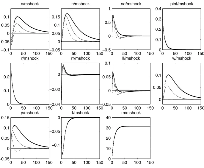
Impulse response functions are presented in figure 3. Here, as opposed to the results for flexible (and exogenous) fees, we list a much wider range of variables. The results we discuss below follow a one standard deviation shock (based on an assumed variance of 10) to the growth rate of money. This induces money growth to jump, then gradually come back to steady state. The money stock thus increases gradually (at a decreasing rate) to its new steady state. Prices, as expected, jump then follow an upward path to settle at a higher equilibrium. The representative lawyer is caught off guard due to the unexpected nature of the shock. But immediately thereafter will attempt to reset her price with probability (1−λ) as a function of her expectations of future prices. Thus, real aggregate entry costs decrease initially, then increase slowly to return to their original steady state. As can be seen in figure 3.
One particularity, of relatively minor interest, is worth noting first. Real entry costs do not immediately drop to their lowest levels, but take three to four periods to do so. This is simply due to the interplay in the dynamics of
entry costs (28) between fbE,t∗ +1 and (Pbt+1−Pbt) in equation (28); since after
the original jump in prices the latter is much larger than the former, fbE,t+1 is
pulled down with respect tofbE,t. As the change in prices quickly diminishes,
the change in entry costs becomes positive, as would be expected of the lawyer trying to cover her higher marginal costs. This mechanism lies at the heart of the sluggishness (slow to move away from steady state) in investment. Secondarily, this also explains why, when labor supply is particularly high, consumption, investment and output exhibit a somewhat surprising jolt in the first period: firms postpone entry while waiting for lawyer fees to come down further, a reaction similar in nature to the inter-temporal tradeoff in investment which we recognized in the model under flexible fees.
Otherwise, figure 3 generally exhibits impulse response functions simi-lar to those of the model under flexible fees with a tradeoff. As discussed already, this is expected. In particular, the sluggishness and persistence of the impulse response functions is inherited from the consumption-investment tradeoff already present in the simpler flexible fees set-up. This similarity is most noticeable in the path of Nt.
One notable difference with earlier results is that the size of the impulse responses diminishes with the wage elasticity of labor supply. As the latter becomes more inelastic, fewer firms are created since labor income is not sufficient to cover as high investment levels without giving up excessive con-sumption. This stands out when comparing two extreme cases (ϕ = 0.25 vs. 4): although investment is more subdued in the first case, consump-tion still dips further than in the second case, in the face of a tighter labor income constraint. As labor supply becomes more elastic, not only can
con-sumers afford to engage in more investment (higher peak in NE,t), but this
investment is concentrated in a shorter time frame (faster return of NE,t to
steady state) to take advantage of the most favorable entry conditions pos-sible. But in all three cases of labor elasticity, investment comes back to its initial steady state before entry costs, due to the inter-temporal shift in firm creation. Thus, the low contemporaneous correlation between entry costs and firm entry, as remarked earlier, continues to hold.
Of paramount importance, output (Yt), consumption and investment are
positively correlated to monetary surprises and display hump shaped patterns similar to those observed empirically and emphasized in Christiano et al. (2005), or Romer and Romer (2004), or even Bergin and Corsetti (2005) and Lewis (2006) concerning investment – or firm creation – in particular. The hump in output is most clear, reaching its apex seven to sixteen quarters (depending on labor elasticity) after the initial shock. Investment peaks faster, as a result of entry costs reaching their trough almost immediately.
Consumption also exhibits a smooth, hump shape, but only after an initial downward and smaller hump. This is due to the decrease in consumption following the monetary shock, as needed to free up funds for investment purposes. Romer and Romer (2004) point out a similar “double hump” pattern, but in the implied response function of output to a monetary shock.15 Of potential importance to central banks, the model results emphasize the long lasting effects that a temporary shock can have. Although the money stock reaches its new steady state after 50 periods, real variables such as consumption, wages, production and GDP come back to steady state after about 100 periods. The actual number of periods is misleading as it is an
artifact of the somewhat debatable choice of parameters; but it remains that the effect of monetary policy is felt for about two times longer than the policy impetus.
Otherwise, the real interest rate,RRt, plays its expected role to clear the
inter-temporal consumption market, as warranted by the Euler equation in bonds. Indeed, the real interest rate is positive when consumption swells and negative when it wanes. Christiano et al. (2005) note that real rates fall after a monetary shock. Our ability to reproduce this result is mixed: real rates do remain in negative territory for most of their time away from steady state, but they surge to positive levels for a short period early on. This is due to the initial negative hump in consumption, and interest rates needing to remain positive for a while in order to pull consumption comfortably above steady state, a result not discussed in Christiano et al. (2005).
One apparent drawback of our model’s simulations is the lack of liquidity effect. This was already a puzzle in traditional New Keynesian models, as pointed out in Gali (2002), which is only able to give rise to a liquidity effect with particular values of risk aversion and money growth autocorrelation. We do not find a liquidity effect probably because inflation jumps too much and too quickly (thus pushing up the nominal interest rate). In and of itself, the lack of sluggishness in inflation is also a relative weakness of our model, yet it follows from assuming flexible prices in the goods market, a direction we took explicitly in order not to cloud our results with excessive exogenous persistence. We thus made the choice of emphasizing the model’s impact on real variables, at the expense of realistic patterns in nominal variables. A possible extension of our model with sticky goods prices would have a better
chance of generating a liquidity effect as well as persistent inflation.
The labor market is in line with empirical findings. The increase in real wages following the monetary shock conforms with one the main stylized facts raised in Christiano et al. (2005). Labor supply (ll on the graphs) increases as expected with the real wage, ωt, as needed to attract labor to satisfy the
greater number of firms and higher aggregate output. Almost by definition, the effect diminishes with the wage elasticity of labor supply. Interestingly, though, labor supply comes back to steady state relatively quickly (by even overshooting it). This is due to the decreasing marginal utility of a rising level of consumption, which peaks only after real wages do (recall the opposing effect of consumption and real wages on labor supply). In passing, note that the continued positive level of output even while labor supply is back at its steady state comes from a higher degree of available varieties; once again, this feature underlines the fact that our variables are given in welfare-relevant terms. We revisit this result in our robustness checks.
Lastly, we note that the extent and duration of all the above-mentioned impulse response functions diminish with the degree of price stickiness, λ. At the extreme, when λ = 0, we are back in the flexible fee world in which real entry costs are unaffected by monetary policy. As a result, none of the real variables budge and monetary shocks only affect prices.16
5.3
Robustness checks: changing the love of variety
We focus here on the role of consumers’ love of variety. In the results dis-cussed above, all simulations were run using ξ = 1/(θ−1), as in the classic Dixit-Stiglitz (1977) case. Thus, the impulse response functions represent
welfare-relevant variables. But not all statistical agencies account for variety in their published indices. And those that do, like in the U.S., do not do so at the frequency inherent in our simulations (1 period = 1 quarter). Thus, on the one hand, it may be more realistic to work with smaller ξparameters. On the other hand, for the purposes of welfare analysis, it may be warranted to consider a strong preference for variety, as seems to be the case in indus-trial economies. To illustrate the effect of changes inξ, we present results for three iterations of ξ: 0, 1/(θ−1) and 0.6 (about twice 1/(θ −1)). Results appear in figure 4.
Generally, a small value ofξshaves off a significant part of the rise in con-sumption, investment, and output. This is as expected. The large upswings in these variables were in part driven by the diversity of product offerings. As variety is valued less (a lowerξ), a unit of expenditure on a good provides less consumption-based utility. Thus, consumption and investment peak lower, contributing to a flatter output curve. On the contrary, as ξ increases, the effects of a monetary shock are magnified considerably.
One particular feature is worth mentioning: the correlation between out-put and labor supply grows as ξ decreases. When love of variety is null, output is only a function of labor employed, and no longer responds to the number of firms (as can be seen in equation 19). In addition, as ξ decreases, labor supply is increasingly dependent on consumption at the expense of real wages, since the latter no longer responds to the number of firms (as can be seen in equation 17). Thus, ξ = 0 represents the case when labor sup-ply most overshoots its return to steady state, thereby also pushing output briefly below steady state after an initial and much larger expansion.
Lastly, we note that changes inξ affect only real variables, leaving nom-inal variables nearly unchanged. Again, this is due to our assumption of adjustable goods prices, whereby variations in nominal variables are domi-nated by the monetary shock, as in a flexible price setting.
We generally remain agnostic as to the correct choice of ξ, but until statistical agencies pay closer attention to variety, we note that the crux of our results, namely the hump shaped patterns in real variables following a monetary shock, remain true despite changes to the love of variety.
6
Conclusion
We found motivation for this paper among the quickly growing empirical lit-erature pointing to the central role of firm entry and exit as an endogenous propagation mechanism for macro-economic shocks. More specifically, we were encouraged by recent empirical and anecdotal findings emphasizing the positive correlation between firm entry and monetary expansions. We were also motivated by the challenge of offering an alternative modeling response – less dependent on exogenous rigidities – to the New Keynesian models’ dif-ficulty of generating persistent and sluggish responses to monetary surprises. In response to these stimulations, we developed a monetary model where firm entry is endogenous. To enter, monopolistically competitive firms must pay a sunk fee, then wait one period before being able to produce. The payment of this fee is intended to be synonymous with costs such as the setting-up of operations, hiring, R&D, marketing or other activities. Entry is regulated by consumers who optimize spending between consumption and investment in new firms. This introduces an endogenous source of inertia
in the model, as consumers aim to smooth consumption and therefore do not immediately succumb to the requests for funding when entry conditions suddenly turn favorable.
In our model, monetary policy shocks directly affect the cost-benefit anal-ysis preceding entry, by influencing Tobin’s Q, or the ratio of expected future profits to the cost of entry. We do so by assuming that entry costs are set a la Calvo (1983), while goods prices remain flexible throughout the analysis. In doing so, we were inspired by a wide body of research in the IO literature pointing to the relevance of sunk costs for firm entry.
As a result of this apparatus, monetary policy has significant real effects, as shocks generate persistent, as well as hump shaped responses of consump-tion, investment, output and the number of firms. This is as observed in the data (see, for instance, Christiano et al., 2005, or Romer and Romer, 2004), but as generated only with significant difficulty, or with a series of assumed exogenous rigidities, in traditional New Keynesian models. Our model therefore stands apart as presenting minimal nominal rigidities and simple microfounded dynamics underlying a new channel for the transmission of monetary policy.
References
[1] Benassy, J.-P., 1996. “Taste for Variety and Optimum Production Pat-terns in Monopolistic Competition,” Economics Letters 52, 41-47. [2] Bergin, P. R. and G. Corsetti, 2005. “Towards a Theory of Firm Entry
and Stabilization Policy,” NBER Working Papers No. 11821.
[3] Bilbiie, F., F. Ghironi and M. J. Melitz, 2005. “Endogenous Entry, Prod-uct Variety and Business Cycles,” mimeo, University of Oxford, Boston College and Princeton University.
[4] Bilbiie, F., F. Ghironi and M. J. Melitz, 2007. “Monetary policy and business cycles with endogenous entry and product variety,” forthcoming in NBER macroeconomic annual.
[5] Bernard A. B., J.Eaton, J. B. Jensen and S. Kortum, 2003. “Plants and Productivity in International Trade,” The American Economic Review 93, 1268-1290.
[6] Blanchard, O. and L. F. Katz, 1999. “Wage dynamics: Reconciling the-ory and evidence.” American Economic Review 89, 69-74.
[7] Broda, C. and D. E. Weinstein, 2004. “Variety Growth and World Wel-fare,” American Economic Review 94, 139-144.
[8] Broda, C. and D. E. Weinstein, 2006. “Globalization and the Gains from Variety,” The Quarterly Journal of Economics,121, 541-585.
[9] Calvo, G., 1983. “Staggered prices in a utility-maximizing framework,” Journal of Monetary Economics 12, 383-98.
[10] Casares, M., 2002. “Time to Build Approach in a Price, Sticky-Wage Optimizing Monetary Model,” ECB Working Paper No. 147. [11] Chatterjee, S. and R. W. Cooper, 1993. “Entry and Exit, Product
Va-riety and The Business Cycle,” NBER Working Paper No. 4562. [12] Clarida, R., J. Gali and M. Gertler, 2001. “Optimal Monetary Policy
in Closed Versus Open Economies: An Integrated Approach,” NBER Working Paper No. 8604.
[13] Chari, V. V., P. J. Kehoe and E. R. McGrattan, 1997. “Monetary Shocks and Real Exchange Rates in Sticky Price Models of International Busi-ness Cycles,” NBER Working Paper No. 5876.
[14] Chen, N., J. Imbs and A. Scott, 2006. “The Dynamics of Trade and Competition,” Mimeo, HEC Lausanne.
[15] Christiano, L., M. Eichenbaum and C. Evans, 2005. “Nominal Rigidities and the Dynamic Effects of a Shock to Monetary Policy,” Journal of Political Economy 113, 1-45.
[16] Christiano, L., M. Eichenbaum and C. Evans, 1999. “Monetary Policy Shocks: What Have We Learned, and To What End.” In: Taylor, J. and Woodford, M. (Eds.)Handbook of Monetary Economics, Vol. I. Oxford: Elsevier, 65-148.
[17] Corsetti, G., P. Martin and P. Pesenti, 2005. “Productivity Spillovers, Terms of Trade and the Home Market Effect,” NBER Working Paper No. 11165.
[18] Davis, S. J., J. C. Haltiwanger and S. Schuh, 1998. Job Creation and Destruction. Boston, Massachusetts: The MIT Press.
[19] Dixit, A. and J. Stiglitz, 1977. “Monopolistic Competition and Optimum Product Diversity,” American Economic Review 67, 297-308.
[20] Fuhrer, J. and G. Moore, 1995. “Inflation persistence.” Quarterly Jour-nal of Economics CX, 127-160.
[21] Gali, J., 2002. “New Perspectives on Monetary Policy, Inflation, and the Business Cycle,” NBER Working Paper No. W8767.
[22] Gali, J. and M. Gertler, 1999. “Inflation Dynamics: A Structural Econo-metric Analysis,” Journal of Monetary Economics 44, 195-222.
[23] Ghironi, F. and M. J. Melitz, 2005. “International Trade and Macroe-conomic Dynamics with Heterogeneous Firms,” The Quarterly Journal of Economics 120, 865-915.
[24] Goodfriend, M. and R. King, 1998. “The New Neoclassical Synthesis and the Role of Monetary Policy,” Federal Reserve Bank of Richmond Working Paper No. 98-5.
[25] Hopenhayn, H., 1992a. “Entry, Exit and Firm Dynamics in Long Run Equilibrium,” Econometrica 60, 1127-1150.
[26] Hopenhayn, H., 1992b. “Exit, Selection, and the Value of Firms,” Jour-nal of Economic Dynamics and Control 16, 621-653.
[27] King, R. G. and S. T. Rebelo, 2000. “Resuscitating Real Business Cy-cles,” NBER Working Papers No. 7534.
[28] Lewis, V., 2006. “Macroeconomic fluctuations and firm entry,” mimeo, Catholic University Leuven.
[29] Mash, R., 2002. “Monetary Policy with an Endogenous Capital Stock when Inflation is Persistent,” Oxford University Discussion Paper Series No. 108.
[30] Melitz, M. J., 2003. “The Impact of Trade on Intra-Industry Reallo-cations and Aggregate Industry Productivity,” Econometrica 71, 1695-1725.
[31] Pencavel, J., 1986. “Labor Supply of Men: A Survey.” In: Ashenfel-ter, O. and Layard, PRG (Eds.) Handbook of Labor Economics, Vol. I. Oxford: Elsevier, 3-102.
[32] Romer, C. and D. Romer, 2004. “A New Measure of Monetary Shocks: Derivation and Implications,” American Economic Review 94, 1055-1084.
[33] Rotemberg, J. and M. Woodford, 1992. “Oligopolistic Competition and the Effects of Aggregate Demand on Economic Activity,” Journal of Political Economy 100, 1153-1207.
[34] Shaked, A. and J. Sutton, 1987. “Product Differentiation and Industrial Structure,” Journal of Industrial Economics 36, 131-146.
[35] Stebunovs, V., 2006. “Finance as a barrier to entry in dynamic stochastic general equilibrium,” PhD dissertation, Boston College.
[36] Sutton, J., 1991. Sunk Costs and Market Structure. Cambridge, Mas-sachusetts: The MIT Press.
[37] Woodford, M., 2005. “Firm-Specific Capital and the New-Keynesian Phillips Curve,” NBER Working Paper No. 11149.
[38] Woodford, M., 2003. Interest and Prices: Foundations of a Theory of Monetary Policy. Princeton: Princeton University Press.
0 50 100 150 !1 !0.5 0 0.5 c/tradp/fshock 0 50 100 150 0 0.2 0.4 0.6 0.8 1 n/tradp/fshock 0 50 100 150 0 1 2 3 4 5 6 7 ne/tradp/fshock 0 50 100 150 !1 !0.8 !0.6 !0.4 !0.2 0 f/tradp/fshock
Figure 1: Benchmark model in flexible prices, variant I: Temporary shock tofE,t with autoregressive coefficient 0.9. The responses exhibit endogenous
0 50 100 150 0 0.1 0.2 0.3 0.4 0.5 c/flexp/fshock 0 50 100 150 0 0.5 1 1.5 n/flexp/fshock 0 50 100 150 0 20 40 60 80 100 ne/flexp/fshock 0 50 100 150 !1 !0.8 !0.6 !0.4 !0.2 0 f/flexp/fshock
Figure 2: Benchmark model in flexible prices, variant II: Temporary shock to fE,t with autoregressive coefficient 0.9. The impulse responses exhibit no
0 50 100 150 !0.1 !0.05 0 0.05 0.1 c/calvo/mshock 0 50 100 150 0 0.1 0.2 n/calvo/mshock 0 50 100 150 !0.5 0 0.5 1 ne/calvo/mshock 0 50 100 150 0 0.1 0.2 0.3 0.4 pinf/calvo/mshock 0 50 100 150 0 0.1 0.2 r/calvo/mshock 0 50 100 150 !0.04 !0.02 0 0.02 rr/calvo/mshock 0 50 100 150 !0.05 0 0.05 0.1 0.15 ll/calvo/mshock 0 50 100 150 !0.02 0 0.02 0.04 0.06 0.08 w/calvo/mshock 0 50 100 150 !0.05 0 0.05 0.1 0.15 y/calvo/mshock 0 50 100 150 !0.1 !0.05 0 f/calvo/mshock 0 50 100 150 0 10 20 30 40 m/calvo/mshock
Figure 3: Temporary shock to money growth, with autoregressive coefficient 0.9 in a model with Calvo pricing in entry costs and different wage elasticities of labor supply. Solid line: ϕ = 0.25, hyphenated line: ϕ = 1, dotted line: ϕ = 4.
0 50 100 150 !0.1 !0.05 0 0.05 0.1 c/mshock 0 50 100 150 !0.05 0 0.05 0.1 0.15 n/mshock 0 50 100 150 !0.5 0 0.5 1 ne/mshock 0 50 100 150 0 0.1 0.2 0.3 0.4 pinf/mshock 0 50 100 150 0 0.1 0.2 r/mshock 0 50 100 150 !0.04 !0.02 0 rr/mshock 0 50 100 150 !0.05 0 0.05 0.1 ll/mshock 0 50 100 150 0 0.05 0.1 w/mshock 0 50 100 150 !0.05 0 0.05 0.1 0.15 y/mshock 0 50 100 150 !0.1 !0.05 0 f/mshock 0 50 100 150 0 10 20 30 40 m/mshock
Figure 4: Temporary shock to money growth, in a model with Calvo pricing in entry costs, ϕ = 1 and different degrees of love of variety. Hyphenated line: ξ = 0 (no love of variety), solid line: ξ = 1/(θ−1) (the Dixit-Stiglitz case), dotted line: ξ= 0.6 (high love of variety).