Kent Academic Repository
Full text document (pdf)
Copyright & reuse
Content in the Kent Academic Repository is made available for research purposes. Unless otherwise stated all content is protected by copyright and in the absence of an open licence (eg Creative Commons), permissions for further reuse of content should be sought from the publisher, author or other copyright holder.
Versions of research
The version in the Kent Academic Repository may differ from the final published version.
Users are advised to check http://kar.kent.ac.uk for the status of the paper. Users should always cite the published version of record.
Enquiries
For any further enquiries regarding the licence status of this document, please contact:
researchsupport@kent.ac.uk
If you believe this document infringes copyright then please contact the KAR admin team with the take-down information provided at http://kar.kent.ac.uk/contact.html
Citation for published version
Oberoi, Jaideep S (2017) Interest rate risk management and the mix of fixed and floating rate debt. Journal of Banking and Finance, 86 . pp. 70-86. ISSN 0378-4266.
DOI
https://doi.org/10.1016/j.jbankfin.2017.09.001
Link to record in KAR
http://kar.kent.ac.uk/63376/
Document Version
Interest rate risk management
and the mix of fixed and floating rate debt
Jaideep Oberoi
McGill University, Desautels Faculty of Management, 1001 Sherbrooke Street West, Montreal, Quebec, H3A 1G5, Canada.
and
University of Kent, Kent Business School, Canterbury CT2 7PE, United Kingdom. Tel: +44 1227 82 3865. Email: j.s.oberoi@kent.ac.uk
Abstract
We analyze the after-swap mix of fixed and floating rate debt in a sample of non-financial firms, using hand-collected data from a window of time when derivative positions were included in accounting disclosures. To motivate the analyses, we present a simple theoretical model that highlights the special features of interest rate risk. Consistent with the theory, we find that firms that issue more fixed rate debt have higher liquidity ratios and lower operating income ratios. We also document that individual firms actively vary the proportion of their fixed rate debt to a strikingly high extent. There is a debate as to whether such variation should be interpreted as hedging or speculation. We show that the firms more actively varying their debt mix respond to different hedging motives than those with low activity. We then empirically motivate an alternative indicator of speculative activity: co-variation between ex-post profitability of financial decisions and operating results.
JEL Code: G32
Key words: Risk management; Interest rate risk; Fixed rate debt; Active hedging; Speculation.
Acknowledgements
This paper has developed from work done for my PhD thesis under the supervision of Peter Christoffersen and Amrita Nain, and I am extremely grateful to them for their guidance, support, and contributions, both intellectual and financial (towards data collection), to this research. This paper has benefitted greatly from the comments and suggestions of the editors and reviewers and I am grateful to Carol Alexander (the Editor) and the anonymous referees for their thoughtful reviews. I am also grateful for helpful comments from Tom Aabo, Ron Anderson, Murillo Campello (FMA Doctoral Consortium), Tolga Cenesizoglu, Susan Christoffersen, Hitesh Doshi, Marc Georgen, Jim Griffin, Adolfo de Motta, Lawrence Kryzanowski, Kristian Miltersen, Melania Nica, and seminar participants at McGill University, University of Kent and the University of Guelph. All errors are my responsibility.
[1]
1. Introduction
In this paper, we examine the association between hedging motives and the mix of fixed and floating rate debt in individual firms. Both types of debt present different forms of interest rate risk – floating rate debt exposes a firm’s net profits to variable interest costs, while fixed rate debt impacts the firm’s future borrowing and investment capacity through changing liability or leverage levels. We ask what motivates firms to choose one type of debt over another, and then to vary the mix over time. Can we interpret the choice of a particular mix, or the extent of its variation, as an indicator of risk-reducing or risk-increasing behavior by managers? We address these questions by analyzing a decade-long hand-collected sample that incorporates the net effects of interest rate swaps on the final mix of debt in the firms.
The aim of this paper is to contribute to the literature on corporate risk management in nonfinancial firms, specifically on the subject of interest rate risk. Previous papers have found some evidence that the choice of borrowing in firms is not consistent with hedging motives. Bodnar et al. (1998) report that over half of firms responding to their survey on derivatives usage admitted to allowing their view of future interest rates to affect their interest rate derivative position (direction, size and/or timing). Faulkender (2005) finds that debt issuances by a sample of firms in the chemical industry may be driven by myopic market-timing objectives, rather than hedging motives. Chava and Purnanandam (2007) find for a cross-section of firms that the vega from CFOs' compensation is positively related to the proportion of floating rate debt. Chernenko and Faulkender (2012) study a panel of interest rate exposure data to separate out between- and within-firm variation, classifying the first type of variation as arising from hedging motives and the second as speculation. They present evidence of both hedging and speculation, as well as of income smoothing by managers. This complex picture is representative of the difficulty in
pinning down firms’ motives in the absence of a benchmark hedging rule for choosing the mix of
debt.1 We study whether both the level and variation of the mix of fixed and floating rate debt
1 Alternative explanations for interest rate choice at debt issuance include the signaling model of Guedes and
Thompson (1995). They argue that, as expected inflation volatility increases, floating rate debt becomes a better hedge for the firm, making it less useful for firms to use as a signal of quality. On the other hand, Campbell (1978) and Santomero (1983) considered debt issuance choice from the perspective of bank liquidity dynamics. Since their introduction in response to high inflation in the 1970s, the share of long-term floating rate instruments in the markets
[2]
are associated with risk management incentives through a series of tests.
Our findings suggest that neither fixed nor floating rate debt can be unconditionally classified as risk increasing. In addition, we find that firms that vary their mix more than others may be doing so for hedging motives along a different dimension than the less active firms. This helps us to reconcile some of the mixed findings in the literature.
Our work is also related to the wider literature on corporate risk management in two ways. Firstly, we rely on variables identified in the literature as indicators of or proxies for the strength
of firms’ risk management incentives. Secondly, we are guided by the emphasis on data collection in the literature. There is a rich literature on corporate risk management presenting mixed evidence on whether risk management adds value, and on which of the risk management theories are supported in the data. These include, among others, Nance, Smith and Smithson (1993), Mian (1996), Tufano (1996), Géczy, Minton and Schrand (1997), Schrand and Unal (1998), Haushalter (2000), Allayanis and Weston (2001), and Knopf, Nam and Thornton (2002). The above studies rely on survey data and/or alternative indicators of derivative usage (including notional values), and Aretz and Bartram (2008) discuss the complex picture of risk management activity that does not solely rely on derivatives. Brown (2001) and Bartram (2008)
conduct case studies of a single firm’s foreign exchange risk management; while Adam and Fernando (2006) show that speculation using derivatives is profitable in the gold industry. Graham and Rogers (2002) recognize that the notional value of derivatives used by a firm is often not linked to the extent of hedging or more specifically the net exposure from derivative positions. This is because firms typically do not buy and sell over the counter derivatives, but take offsetting positions when they wish to close a position. They address this data issue by using net exposures from derivatives. More recently, Campello et al. (2011) demonstrate the channels (financial contracting and real investment) through which hedging adds value to the firm. The possibility for firms to use alternative methods for managing risk is demonstrated by Petersen and Thiagarajan (2000) and Kim et al. (2006), and although they study other risks, this is particularly important for interest rate exposures. Servaes et al. (2009) also find that the impact
the rise of liquid markets in swaps has made the choice at issuance less important when considered exclusively. Similarly, work cited later in the paper shows that constraints from the source of debt (bank or public) can also be alleviated with swaps.
[3]
of derivatives on the final interest rate mix is relatively small.
One challenge with the data needed for tests of risk management theories has been the versatility of derivatives and their accounting treatment. However, for a period of transition lasting approximately a decade, accounting disclosure regulations offered strong incentives for firms to provide details about their derivative positions in footnotes to their financial statements. During the 1990s, companies in general reported both the face value and direction of derivative contracts in their annual reports, thus presenting an opportunity to collect arguably the best available data on firms' interest rate positions. New rules designed to bring the contracts onto the balance sheet then effectively altered these disclosure requirements by 2001 (see also Graham and Rogers 2002). The development of these rules is recounted in the Appendix. We exploit this window created by regulatory changes to obtain our data on both interest rate derivatives and debt exposures. We are therefore able to overcome some of the data limitations faced in classifying firms, by recording their actual positions rather than derivative usage proxies.
We first examine the mix of fixed and floating rate debt, and show that it is jointly associated with the nature of constraints endogenously chosen by firms. When firms have more fixed rate debt, they have relatively lower operating profits, but also have more liquid assets – hence protecting them from decreases in interest rates that would lead to future financing constraints. This result is consistent with Acharya et al. (2007) and Almeida et al. (2011), who study the effect of future financing constraints (a motive for risk management) on joint determination of policies of the firm. Conversely, when firms have more floating rate debt they have higher operating profits. One interpretation of this association is simply that the operating profits cushion the firms from interest rate variations. However, this result is also consistent with
structural models of the firm used in debt pricing, that link a firm’s asset value to incentives for
holding floating rate debt, on average (e.g. Longstaff and Schwartz, 1995).
Next, we study the time series of the proportion of fixed rate debt of individual firms. The empirical risk management literature often assumes that firms’ underlying exposures to risk factors imply stable target proportions for financial variables like leverage, or even the mix of fixed and floating rate debt. By extension, if a firm varies the mix of its debt more often than another, it should signify changing exposure, higher sensitivity to risk, or speculative activity. Chernenko and Faulkender (2012) make a significant advance in disentangling hedging and
[4]
speculation by using panel data. They do so by assuming the existence of a stable ‘target’
proportion of fixed rate debt for each firm. We classify firms by the extent of variation of their proportion of fixed rate debt over time, into those that are more or less active. If being active implies speculative or other forms of deviation from an optimal target, we expect to find evidence of value destruction or lower hedging imperatives in the relatively more active firms. We examine the above hypotheses in turn, through a number of tests. We first examine the
relationship between firms’ cash flows and interest rates. We test whether, on average, the
interest rate exposures of active firms differs from those of less active ones. We find the
difference between the average sensitivities of the two groups’ operating profits to be significant
and negative. Also, on average, the operating profits of active firms vary negatively with interest rate levels. This suggests the existence of incentives to hedge interest rate exposures in active firms. Next, we compare the two groups of firms on other characteristics that the literature considers as motives for hedging. The more active firms are smaller on average than the less active firms and have higher market-to-book ratios, but the two groups are not different in terms of investment or research and development expenditure ratios. Overall, we find no evidence that being active is by itself an indicator of speculative or ‘non-hedging’ behavior.
The above analysis complements the findings of Chernenko and Faulkender (2012) on the use of swaps for income management to the extent that both analyses involve the identification of non-hedging motives. Chernenko and Faulkender focus on an ex-post approach, which implies that managers transfer accounting income across years when they know what their performance will be.
One may wonder whether the classification between active and inactive firms is even that strong. An important side-effect of this analysis is that we document for the first time the high level of heterogeneity in the extent to which firms vary the mix of debt over time. Not only is there heterogeneity in this variation, the level of variation is striking. For each firm in each year of our eleven-year sample, we calculate the proportion of debt that is subject to fixed rates after accounting for interest rate swaps. We then calculate the range of this proportion over the sample period, i.e. the difference between the maximum and minimum proportion of fixed rate debt for each individual firm. The median of this range is 0.51, showing that more than half the firms switched between having mostly fixed rate debt and mostly floating rate debt, or vice versa.
[5]
One of the additional contributions in this paper is the application of an appropriate estimation methodology, considering that the proportion of fixed rate debt exposure takes values between 0 and 1. The standard linear regression model in such a setting may lead to biased and inconsistent estimates (Cook et al., 2008; McCullagh and Nelder, 1989; Papke and Wooldridge, 1996), so we apply a beta regression instead, which is explained in Section 4.
Having found evidence consistent with hedging motives being linked to various proxies for interest rate exposure choice and variation, we would still like to make an attempt at identifying speculation. To explore an alternative indicator for speculation, we conduct a thought experiment based on purely hypothetical scenarios. The question we ask is, what could we learn if we assumed that firms were attempting to time the market for short term gain?
Our sample extends across varied periods of monetary policy, with sustained episodes of unexpectedly low and high rates, as well as shock increases and decreases in rates. This places us in a position to observe how often a firm increases the share of its fixed rate debt before interest rates go up, or reduces the share of fixed rate debt before interest rates go down.
Capitalizing on this opportunity, we uncover an unexpected association between operating performance of a firm in a given year and the change in its debt mix in the previous year. This finding is consistent with the notion that some managers may be making correlated decisions across all the dimensions of the firm, not optimally, but based on their views on future interest rates. This possible explanation is consistent with the finding in Géczy et al. (2007) that managers selectively choose exposures based on their views rather than specifically setting out to gamble. It is also similar in spirit to that used by Beber and Fabbri (2012), who use unexplained changes in the size of currency derivative positions to identify speculation and associate these actions with behavioral attributes of managers. If this explanation is correct, it points to a potential proxy for identifying firms that speculate over a period of time. Speculators would have a higher absolute value of correlation between the following two dimensions: operating performance, and the financial impact of the change in the debt mix in the previous year.
Underlying the discussion in this introduction and motivating the choice of analyses in this and other papers in the literature, is the issue that theory does not provide us with an optimal benchmark mix of fixed and floating rate debt, with which to compare the empirically observed mix. We began this paper with the argument that the firm trades off two different facets of
[6]
interest rate risk when it chooses the shares of fixed and floating rate debt. In order to help motivate our analysis further, and to link it to the theoretical developments in corporate risk management, we first present a simple model to characterize the form of interest rate risk in the next section.
Overall, we show in this paper that the mix of fixed and floating rate debt is associated with future financing constraints as predicted by theory. In addition, we document striking levels of variation in this mix by individual firms over time. We exploit heterogeneity in the extent of variation to conclude that both types of firms are responding to different hedging incentives, and that being active does not appear to signal speculative motives. The above analyses are discussed in Section 4. In Section 5, by considering the association between financial choices and operational results, we explore a potential approach to distinguish speculators from others. We use Section 3 to describe and summarize the data.
2. Theory and further motivation for tests
Theory offers several justifications for risk management in the context of Modigliani’s and Miller’s (1958) setup. In the presence of asymmetric information (Froot et al., 1993), financial distress costs (Leland, 1998; Purnanandam, 2008) or agency costs (Morellec and Smith, 2007), firms may benefit from smoothing cash flows to avoid deadweight losses from underinvestment or liquidation. Independent of the source of market distortion, financing constraints arise in states with profitable investment opportunities, generating a motive for hedging. The effect of such future financial constraints is discussed in, for instance, Acharya et al. (2007) and Almeida et al. (2011). Other sources of risk management incentives include convex tax schedules and managerial concerns for their own wealth or career (Breeden and Viswanathan, 1998; DeMarzo and Duffie, 1991, 1995; Smith and Stulz, 1985; Stulz, 1984). Further, strategic implications of hedging are explored in Adam et al. (2007) and Adam and Nain (2012). In this section we attempt a simple characterization of the tradeoffs generated by interest rate risk assuming one or more of these justifications hold.
It is clear that more than one aspect of the firm (revenues, costs, financial value in terms of future prospects) may be related to variations in a market variable such as the short rate. While any firm may be exposed to interest rate risk in this sense, the presence of debt modifies this exposure. For an indebted firm, potential up and down moves of interest rates also act through the debt, and
[7]
the effect depends on whether the debt is at fixed or floating rates. A decrease in the interest rate
raises the value of fixed rate debt and thus reduces a firm’s borrowing capacity, ceteris paribus.
An increase in rates raises interest payments on floating rate debt, thereby directly reducing income and internal resources. As both fixed and floating rate debt expose the firm to the risk of suboptimal investment choices, a firm could be seen to opt for a mix that trades off the two manifestations of risk given their specific exposure. We are interested in this particular choice. In this section, we propose a simple framework that would help to identify the salient features of interest rate risk for nonfinancial firms, and place it in the context of existing risk management theory.
2.1 A simple adaptable characterization of interest rate risk
We adapt the information structure from Acharya et al. (2007) to address the fixed versus floating interest rate marginal decision for a firm in a simple setting.
2.1.1 Assumptions
[Insert Figure 1 here] There are three dates in the model (see Figure 1).
At t = 0, the firm takes up a project with uncertain cash flows and partly finances it with debt with face value d on which it must pay coupons at t = 1, 2. The debt is repaid at t = 2. At t = 1, the firm receives a high or low cash flow CH or CL respectively. Here, cash flow refers to the underlying cash flow generated by the assets of the firm, and is in an accounting sense similar to EBIT. Thus, the value of the assets of the firm is inextricably linked with the EBIT, in the sense of Goldstein et al. (2001). On the other hand, the value of equity and debt may vary according to other factors. Also, the one-period risk-free interest rate either rises to rH with probability p or falls to rL with probability (1-p). Cash flows and interest rates are correlated - the probability of a high cash flow in the low interest rate state mirrors that of a low cash flow in a high interest rate state (see Figure 1). The expression for the correlation between cash flows and interest rates is:
,
which can take values between -1 and 1, as long as p is not 0 or 1. This correlation varies across individual firms, and in our stylized example, affects their sensitivity to each type of debt.
[8]
At t = 1, the firm has an opportunity to reinvest its residual cash flow (after paying the debt coupon) in the project to earn a positive NPV return s, such that it is always optimal for the firm to invest. The cash flow at t = 2 depends on the state at t = 1 as follows. We assume there is no further uncertainty in high cash flow states. In low cash flow states, however, the expected return
from the investment is multiplied by a factor , i.e. with a probability
the return could be low enough to bankrupt the firm, while xH is such that (at a minimum)
the bondholder recovers her entire repayment. We may assume that .
We make some further simplifying assumptions, the first of which is that the existing debt has absolute priority over any new debt issued (for instance, at t = 1). As stated above, coupons are paid on debt at both t = 1 and t = 2. If the debt is at a fixed rate, the coupon is the same in both periods. The coupon on the debt issued at t = 1 is the riskless rate on that date. The existence of default risk still implies that the debt is not issued at par. The restriction on financing comes in the form of limited pledgeability of assets (see Acharya et al., 2007). Only a proportion of current and future cash flows may be pledged to the lender, limiting the total face value of debt available.
The calculations for the various quantities in the model are in the Appendix, so that we may concentrate on the key implications of the model.
2.1.1 Implications
If the firm only issues one type of debt with face value d at time 0, and the fixed rate debt is issued at a rate r0, such that rL < r0 < rH, we have the following expressions for the value of the fixed and floating rate debt respectively:
s I x r d r d q p s I x r d r d q p r d q p r pqd r dr D LL L L L LH L H H L H F 1 1 1 , 1 min 1 1 1 1 , 1 min 1 1 1 1 1 1 0 0 0 (1)[9]
s I x r d r d q p s I x r d r d q p r q p pq d r dr D LL L LH L FL 1 1 1 , 1 min 1 1 1 1 , 1 min 1 1 ) 1 1 ( 1 0 0 0 0 0 0 0 0 (2)Comparing expressions in Eqn. 1 and Eqn. 2, we can see that the value of the floating rate debt depends on default probabilities, but is not sensitive to future realizations of the interest rate, whereas the fixed rate debt is in fact subject to both interest rate and default risk.
Consider now the cash-flows to the shareholders in the firm. A firm that has borrowed at a fixed rate expects to receive the following cash flows at time 2:
pq1p 1q
CHdr0
1s
p
1q 1p
q
xH
CLdr0
1s 1 d1r0
(3)The cash-flows to floating-rate borrowers would be
H L
H
H
L
L
L H H H r d s dr C x q p r d s dr C x q p r d s dr C q p r d s dr C pq 1 1 1 1 1 1 1 1 1 1 1 1 0 0 0 0 (4)In this case, the cash flows to shareholders in the case of fixed rate debt depend on default probabilities and the underlying operating uncertainty, but are not affected by interest rate changes. However, floating rate borrowers are affected adversely, particularly in the state with low cash flows and high interest rates coinciding. Two states are more important than others - the low cash flow, low interest rate regime that affects fixed rate borrowers harshly and the low cash flow, high interest rate regime that hurts floating rate borrowers.
Given the unlimited potential for returns from investing at time 1, we now consider the possibility that the firm may increase its investment by borrowing an additional amount. We know that the firm may not commit more than a proportion of its cash balances and expected cash flows as collateral. Hence, in each of the four states at time 1, we can work out the maximum (and in this case optimal) amount of borrowing (when initial debt is fixed). For instance, in the high cash flow, high interest rate state,
H H HH HH r r d s dr C B d 1 ) 1 ( 1 ) ( 1 0 0 1 (5)[10]
Appendix.
The key comparison is the cost of debt ( d1/B1 ) in the low cash flow states when interest rates are high or low. When initial debt is fixed, we can find that
1 (1 ) 1 ) 1 ( 1 1 1 1 0 0 0 1 1 1 1 r d X s dr C x d X s r r r B d B d L L H LL LL LH LH (6)which implies that the cost of new debt for a fixed rate borrower in the low interest rate state is higher than when interest rates are high. On the other hand, when we consider the same comparison in the case of a firm holding floating rate debt, we find that the difference in the cost of debt is positively related to (rH– rL).
Similarly, in terms of debt capacity at time 1 conditional on existing senior debt with face value d, the borrowing capacity of floating rate borrowers is greater than fixed rate borrowers in a low interest rate environment and vice versa.
The key message from this model is that the mix of fixed and floating rate debt that optimizes shareholder value depends on the relative size of EBIT and the relative variation in interest rates and the correlation between EBIT and interest rates, taking into account future investment opportunities (including financial frictions). This helps place the problem in the context of the traditional approaches to corporate risk management,
2.1.2 Empirical guidance
Here we assumed limited pledgeability that could arise from agency costs. These same agency costs can be alternatively modelled as causing external finance to be more costly and to have a convex cost structure. This approach is taken in Froot et al. (1993). They also guide us on how to optimally hedge in such a setting. The answer, which is also adopted in Faulkender (2005) is to smooth the underlying cash flows or the EBIT of the firm. Thus, from a practical perspective, risk management involves hedging to reverse the effects of correlation between operating profits and the variable of interest (e.g. interest rates).
Firms may have different levels of constraints that necessitate greater or lesser hedging motives, and we take these variables from the literature to determine whether a particular choice along the fixed-floating rate debt margin is related to any of these incentives.
[11]
which speaks of the existence of growth opportunities and of financial distress costs as central considerations. For instance, Stulz (1984), Smith and Stulz (1985) and Froot et al. (1993) predict a positive relationship between these variables and hedging activity. On the other hand, Morellec and Smith (2007) show that large firms with low growth opportunities may also reduce risk in order to avoid overinvestment costs. Further, Almeida et al. (2011) show that firms with future financing constraints may have a negative relationship between risk-taking and leverage. These latter papers motivate us to retain liquidity and underlying cash flow (profitability) in the mix of predictors.
3. Data on the mix of fixed and floating rate debt
3.1. Sample selection
The main objective of this exercise was to take advantage of the period when data on both interest rate derivatives and debt were available. For inclusion of a firm in the database, there had to be a history of its annual financial statements available from the 1990s. In order to collect a large enough sample, we first randomly picked companies from the S&P 500 index in 2007. This was purely to obtain a list of firms that had a reasonable likelihood of a financial history being available, and the sample is not intentionally meant to be representative of a particular group of firms. The financial statements were taken from EDGAR SEC filings data (typically starting with the fiscal year 1994), as well as the Lexis-Nexis database for the early 1990s. 100 companies from the S&P 500 index in 2007 were picked, and their statements were read for the financial years 1990 through 2000. Data on their derivatives usage and debt mix were then collected from the footnotes to the statements.
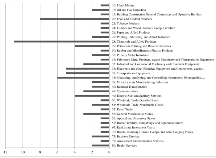
The industry distribution of the firms is quite varied, with 63 different 4-digit SIC categories. To see the distribution over 2-digit levels, please see Figure 2.
[Insert Figure 2 here]
The choice of the sample period is dictated by developments in accounting regulations that created a window in time when data on debt and swaps was jointly available in a manner to allow interpretation of net exposures. These regulations and their impact on data availability are discussed in more detail in the Appendix.
[12]
3.2. Collection of data on derivative and debt positions
The data was collected by a team of research assistants and cross-checked at least once. We used mainly footnotes to the financial statements to collect data on debt and derivatives positions. For derivatives, we collected detailed information on all interest rate derivatives used by each company in each year. We searched the footnotes to the annual statements through the use of multiple search terms in addition to looking for certain sections of the footnotes manually to ensure detailed and accurate data. Our initial experience showed that searching for standard terms such as ‘swap’, ‘cap’, ‘futures’, ‘forward’, ‘floor’, ‘collar’, and ‘hedg’ was not sufficient as companies often use terms such as “interest rate protection agreement” and “interest rate
exchange agreement” to mean the same things. In order to ensure completeness, we read through
the sections that referred to fair value disclosures, risk management, off-balance sheet instruments, and debt, in addition to checking for references to these terms in the management's discussion section of filings. Where companies mentioned the hedging of investments as one of their reasons for using interest rate derivatives, we also read the section on investments. This distinction is important because a swap related to an investment will have precisely the opposite effect to that of a swap related to borrowing. We classified interest rate instruments as either changing the firm's exposure from floating rates to fixed rates or vice versa. By floating to fixed, we mean an instrument that changes the interest rate payments from a floating rate such as USD LIBOR to a fixed USD rate, directly or indirectly. The exposure is always seen from the point of view of a liability, so that an increase in interest rates is a negative development for a firm with floating rate exposure and a positive development if you have fixed rates instead. Similarly, a reduction in interest rates is good if you have floating rates and bad if you have fixed rates. We ignored the use of cross-currency swaps when they were being used to hedge foreign currency exposure unless they were clearly shown to have an effect that would fit them into one of our two main categories, viz. floating to fixed or fixed to floating. Although the firms declare investment hedging ability, they actually rarely have swaps matched to investments. This may be related to hedge accounting reasons, as swaps are relatively long-lived, and the firm is obliged to match it to a particular underlying to benefit from hedge accounting. However, it is easy to demonstrate either type of swap as being a hedge when it comes to debt. Firms state they are hedging the cost of debt when they enter into floating to fixed swaps, and the value of debt when they enter into fixed to floating swaps.
[13]
The level and clarity of the disclosures vary significantly across companies. Some companies report individual contracts, since swaps are usually on large sums and are not very frequent. Other companies only provide aggregate level information on the notional and fair values and the direction of the swaps (fixed to floating or vice versa). This latter format is sufficient for our purposes as long as the underlying item(s), whose exposure is being hedged, are delineated. Effectively, the data gives us a snapshot at the end of each year of the extent to which companies altered the mix of fixed and floating rate debt with the use of derivatives. After collecting detailed information about all the instruments in the disclosures, we aggregated the exposures generated by derivatives into floating to fixed or fixed to floating. Where the disclosures were not sufficiently clear as to assign a direction to the derivative positions, we dropped those companies from our sample. For instance, firms providing only the notional value, but not the direction of swaps, had to be dropped; as did those where merger and acquisition activity made data non-comparable over time. Some firms also had to be dropped because they had no significant debt over the period or because debt data was not clear enough to make a determination of exposure. As a result, we have a final sample containing 82 firms over the eleven-year period.
In the case of debt data, firms typically tabulated existing debt in the footnotes to financial statements along with further descriptions in some cases. We also checked the balance sheet when information on short-term debt was not separately provided in the notes. Classification of exposures on debt data often involved reading forward and backwards in years to where the terms of debt issues were properly reported as being at fixed or floating interest rates. Some companies report debt interest rates after the effect of swaps, and this was taken into account to avoid double counting the effect of swaps while combining the numbers.
In order to obtain the final exposure we took the proportion of debt that was at fixed rates (without including the effect of derivatives) and then adjusted it by the net effect of all swaps. We define this as the variable
In Figure 3, we present some observations about pfix graphically. We first present the variation in this proportion for individual firms (over time) and across firms (in a given year). This variation is also compared with that of the leverage ratio.
[14]
In Panel A of Figure 3, we see that the distribution across firms of both the proportion of fixed rate debt and of leverage is fairly stable from year to year (as is seen from the median, interquartile range and standard deviation). Then, in Panels B and C, we look at how much these variables fluctuated for an individual firm over time – the picture is now strikingly different. Over half the firms in the sample switch between being classified as having mostly fixed rate debt and mostly floating rate debt, or vice versa.
Jointly, the observations in Figure 3 present a puzzle as to the motivation for individual firms to vary their interest rate exposures to such an extent. Further, Panels B and C also reflect significant heterogeneity in how variable the debt mix is for individual firms. Why do some firms vary their debt mix significantly more than other firms, given that the average mix across firms does not change much? To the best of our knowledge, we are the first to highlight the extent of this seemingly idiosyncratic variation in the debt-mix of firms.
3.3. Risk exposure indicators and other derived variables
For an individual firm, the variability of pfix may be captured by its range or its standard deviation over time. In order to understand the determinants of this variation, we separate the firms into two groups based on the coefficient of variation of pfix: Active and Less Active. Firms with their coefficient of variation of pfix in the sixtieth percentile and above are classified as Active, while those with the coefficient of variation below the fortieth percentile are classified as Less Active, leaving out the middle 20% of firms to ensure the groups are sufficiently distinct in terms of activeness. Using the standard deviation of pfix as the classification criterion results in categories that have an overlap of 94%, and other results are similar. This is also the case for the range. The coefficient of variation, defined as the standard deviation divided by the mean, is
more appropriate for capturing comparisons when firms have different average levels of pfix.2
As discussed in the theory section, we collect a set of hedge incentive variables based on the theoretical and empirical literature. We collect data from Compustat on market value, sales, leverage, liquidity, research and development expense, capital expenditure, and profitability measures including cash flow margins and return on assets. In order to examine the channels for profitability better, we also include cost variables in our dataset. Market value (mv) is calculated
[15]
as the product of common shares outstanding in millions (csho) and share price at the close of the fiscal year (prcc_f) in the industrial annual Compustat file. Similarly, we have sales (sale) and total assets (at), leverage is total liabilities (long term debt – dltt, plus debt in current liabilities - dlc) divided by total assets, while research and development expenditure (xrd) and capital expenditure (capx) are normalized by total assets. To avoid differences in reporting interpretations, when carrying out tests, we combine capital expenditure with research and
development expenditure to form a composite measure “capital plus R&D expense ratio,” which
is also normalized by assets.. For liquidity, we define the variable quick ratio as cash plus short term investments (che) divided by current liabilities (lct). Cash flow margins are calculated as operating income before depreciation (oibdp) divided by sales, and return on assets as income before extraordinary items (ib) divided by total assets. Market-to-book ratios are calculated as total assets minus common equity (ceq) plus market value, all divided by total assets. Finally, we also have the ratios Cost of goods sold (cogs) and Sales, General and Administrative Expense (xsga) both normalized by sales. To provide an overview of the firms in the data sample, we first calculate the average for each firm over the sample period of each of the variables. A summary of these averages is in Table I.
[Insert Table I here] We also provide correlations across the variables in Table II.
[Insert Table II here]
4. Understanding the interest rate mix
In this section, we discuss the first two exercises described in the introduction. We start by attempting to determine what risk exposures are associated with the proportion of fixed rate debt, and then study the firm-level variation of pfix over time and its association with risk management incentives.
4.1. Exercise 1: How do hedging considerations affect the proportion of fixed rate debt?
In order to answer this question, we regress the firm-year level pfix on the firm characteristics identified earlier. However, as pfix is a proportion, the use of a linear regression model with pfix as the dependent variable would lead to biased and inconsistent estimates (see, e.g., McCullagh and Nelder, 1989; Papke and Wooldridge, 1996; Cook et al., 2008). As a consequence, we
[16]
follow the strategy proposed by Smithson and Verkuilen (2006) to estimate a Beta Regression Model.
To the best of our knowledge, we are the first to address this particular issue with a robust method. This involves assuming that the pfix is conditionally beta distributed with nonlinear submodels for both the location and dispersion parameters of the beta distribution. Such an approach takes account of the necessary heteroskedasticity of the data (as a bounded variable will have variance changing with location), and also allows us to model the precision of the distribution as a function of the same covariates that predict its conditional mean. It is possible to estimate this model in most standard statistical software – we use the betafit package (Buis et al., 2003) in Stata.
While pfix is distributed along the [0,1] interval, other firm characteristics in our regression have a more conventional distribution shape, making this an appropriate use of the conditional beta regression. The model is reproduced below for the reader’s convenience (following Smithson and Verkuilen, 2006):
Let µ be the location parameter and the dispersion parameter of a beta distribution. Further, let
xi be a row of observations of explanatory variables, including a constant. Then,
where and are parameter vectors. Here, µ is the expected value (or location) of the beta-distributed dependent variable (pfix in this case). The variance of the dependent variable is determined jointly by µ and , through the relation: Var(·) = µ(1 - µ)/(1 + ). This means that, for a given level of µ, higher is associated with lower variance.
Our empirical specification includes the same firm characteristics that are used to proxy risk management imperatives. As we have shown in Figure 3 above, the mean pfix for a single firm may carry limited information, but there is still some variation in the cross-firm average of pfix from year to year that may bias the results, so we also include year dummies among the explanatory variables. These year dummies effectively account for general market conditions.
[17]
The results of this regression in Table III show that firms with higher profitability or operating cash flows tend to have a lower pfix while those with higher short-term liquidity (quick ratio) tend to have a higher pfix. This is consistent with the argument that financially constrained firms would hold more liquid reserves. The notion of constraint here is the future borrowing capacity of the firm. A firm with more fixed rate debt exposes itself to the risk of increased leverage,
hence endangering borrowing capacity – such a firm holds more cash and short-term assets as a
hedge. On the other hand, firms with high operating cash flows would face a reduced constraint. In other words, we can see that the choice of issuing more fixed or floating rate debt is linked to other factors affecting the firm, and these change over time. Whether the choice of debt type is determined by the liquidity and profitability of the firm or vice versa is not of central importance
– theory suggests that these would be jointly determined.
From the analysis, we also see that higher leverage is associated with lower pfix. This does not contradict the arguments above, but may also be linked to an alternative explanation. Kahl et al. (2013) argue that firms tend to borrow short-term funds (such as, by issuing commercial paper) for the purpose of making large investments or financing acquisitions. The fact that the leverage-pfix relationship does not appear to hold unconditionally offers increases in short-term borrowing as a potential explanation.
Higher leverage is also linked to higher dispersion in the pfix, suggesting that more extreme values of pfix would be seen in higher leverage firms. This conditional finding is consistent with the argument that firms jointly determine their exposure in consideration with a combination of factors and it would be inaccurate to assume an unconditional link between leverage and the level of pfix or its variation. Sales and quick ratio are marginally significant for the dispersion parameter, with higher sales reducing dispersion and a higher quick ratio increasing it. This is consistent with the view that not all firms are maintaining liquidity as a response to constraints, and some may have other motives for holding short-term assets. This would lead to more variability in the choice of pfix for firms with high liquidity.
4.2. Exercise 2: Variation of pfix and risk management
The next question in this paper is whether high variation in pfix by individual firms can be is linked to hedging or speculation. In this subsection, we compare the strength of hedging incentives between the two groups of firms. We first test for differences in the sensitivity of the
[18]
firms’ operating cash flows to interest rates. We then compare them using both univariate tests and multiple regression with respect to their average characteristics over the sample period. 4.2.1. Are Active firms’ operating cash flows more sensitive to interest rates?
The primary candidate for hedging motives is based on the sensitivity of the firm's underlying cash flows (operating profits) to interest rates, as discussed in Section 2. This theory predicts that the firm would try to adopt a hedge ratio that will allow it to have sufficient internal cash in case investment opportunities arise (see Froot et al., 1993).
Faulkender (2005) obtains firm-by-firm estimates of the ‘betas’ of cash flows with respect to
interest rates – these betas could then be used to proxy for hedge ratios and determine whether
firms should be taking on relatively more fixed or floating rate debt. Positive correlations imply that the firm may be partially naturally hedged against interest rates, while negative correlation suggests that the firm is exposed to greater interest rate risk. We would like to know if Active firms have cash flows more correlated to interest rates than Less Active firms. McNulty and Smith (1998) report a majority of the coefficient estimates for firm-by-firm regressions of cash flows on interest rates are statistically insignificant, although the point estimates vary between -16 and +20. Further, they record high serial correlation in the variables. In order to address these concerns, we group all firms into a single panel regression, using data over all the quarters from
January 1989 through December 2001.3 The dependent variable is operating profits/book assets
as in earlier papers, regressed on its own lag, LIBOR, a dummy for the Active group, and its interaction with LIBOR to estimate the slope differences. The inclusion of the lagged dependent variable is clearly important given the high serial correlation in operating profits. To account for firm-specific characteristics, we use a fixed-effects specification. The regression results are presented in Table IV for the following specifications:
it t i t t i i
it CF LIBOR Active LIBOR u
CF 0, 1 ,12 3 * (1)
Since the mean cash flow dummy would lead to collinearity in the fixed effects regression, this specification provides us with estimates only of the difference between the sensitivities of the cash flows of the Active group with that of the Less Active group. Although the fixed-effects
3 In our sample too, the individual regressions lead to statistically insignificant estimates of beta in too many cases.
[19]
specification is supported by a Hausmann test, we also report a random-effects regression specified as it i t i i t t i
it CF LIBOR Active Active LIBOR u
CF 01 ,12 3 4 * (2)
which is estimated by the Feasible Generalized Least Squares method. In both cases, we report p-values based on clustered (by firm), robust standard errors.
[Insert Table IV here]
We find that, conditional on past profits, Active firms’ profits vary negatively with interest rates, while those of Less Active firms have a marginally positive relationship with the level of LIBOR. The net sensitivity for Active firms is -0.089 + 0.053 = -0.036 from the fixed-effects regression, and similarly -0.037 from the random effects specification. Contrary to the idea that more activity is a sign of speculation, these regressions suggest that Active firms have operating profits that are relatively more exposed to interest rate risk.
We examine further why firms vary their interest rate mix so widely, when we compare other predicted characteristics for hedgers between the two categories of firms.
4.2.2. Other risk exposure indicators and higher activity
First we calculate the average over the entire sample period for each firm of the characteristics listed in Section 3.3. These averages are summarized in Table V.
[Insert Table V here]
In the last two columns of Table V, we report the differences in the average firm characteristics between the two categories of firms, i.e. Active - Less Active, with the p-values below each difference. The results of the univariate tests are inconclusive.
The fact that Active firms are smaller and have higher market-to-book ratios than Less Active firms would theoretically point to activity as being an indicator for hedging behavior based on the asymmetric information (leading to costly external financing) argument. That Active firms have lower leverage and higher liquidity may also be consistent with this argument, but the actual rate of capital expenditure or research and development expenditure in Active firms is not different from that in Less Active firms over the eleven-year period. Perhaps the findings of lower leverage fit better with the overinvestment avoidance argument of Morellec and Smith
[20]
(2007), but then we are faced with the lower size and higher market-to-book ratios of Active firms as contradictions.
Similarly, the Less Active firms can be seen to have hedging incentives from financial distress costs based on their higher leverage and lower liquidity. Does this imply that different types of hedging motives necessitate different hedging strategies? In other words, do smaller firms with growth options have a different policy towards interest rate risk than those that may face greater financial distress costs?
Our next step is to examine the above questions using multiple regression. In Table VI, we present the estimates from a probit regression in which the dependent variable is 1 if the firm is classified as Active, and 0 otherwise. The regressors include all the firm characteristics (we drop market value and total assets in favor of sales as a size proxy). We use heteroskedasticity robust standard errors and report the p-values below the estimates. The estimates reported are not the raw estimates, but the marginal effects estimated at the mean of the explanatory variables.
[Insert Table VI here]
Most of the univariate results survive under multiple regression, still offering conflicting evidence for risk management theory. Firms are likely to vary their interest rate mix more when they have lower sales and (with a weak significance) lower leverage along with higher market to book ratios. Are these firms the hedgers predicted by the combined complementary arguments in Smith and Stulz (1985) and Morellec and Smith (2007), aiming for a target mix of debt? The overinvestment avoidance argument is also supported by the fact that Less Active firms have higher sales, general and administrative expense ratios combined with weakly higher operating profit margins, a potential indicator of the firms’ relative efficiency. Once again, the flip side of the results points to smaller firms with more growth opportunities and lower leverage being
Active – the very firms predicted by asymmetric information considerations to be hedgers.
To recap the findings from this section, an optimal mix of debt can only be interpreted as being jointly determined by other policies and exposures of the firm, and hence to be varying significantly for some firms over time. Thus, activity itself, or deviation from a mean level of fixed rate debt, is just as likely to be consistent with optimal hedging strategy as maintaining a constant level. It appears that Active and Less Active firms face distinct types of hedging motives. Active firms are smaller in size with lower leverage and higher growth opportunities, and their
[21]
operating profit margins are negatively associated with interest rates. As firms get bigger and have lower growth opportunities and higher leverage, they are Less Active, and their cash flow margins are not very sensitive to interest rate levels. We have found evidence that firms with different types of hedging incentives adopt different approaches to varying their interest rate mix.
5. Identifying hedging or speculation
Despite using finer proxies, we have not yet found significant evidence consistent with speculation by managers as reported in the survey findings cited in Section 1. We know that, ceteris paribus, if a firm reduces its pfix by the end of year t, and interest rates fall during year t+1, the firm will face a lower average interest expense in year t+1 than would have been the case under the (higher) pfix that prevailed at the beginning of year t. A similar outcome will arise from an increase in pfix in advance of a rise in interest rates. This specific marginal effect will be reflected in the net profit reported in the financial statement, but not in the operating profit. Based on this observation, we adopt a thought experiment in this section to seek any hints supporting the presence of market timing by managers.
We begin by making the extreme assumption that all managers base their marginal interest rate choice (viz. change in pfix) on their view of future interest rates. What follows in this paragraph is one possible sequence of thoughts based on this extreme assumption. If this assumption were universally true, we could separate firms into two groups based on whether they made an ex-post
“profitable” choice, e.g. chose to increase pfix when interest rates rise in the following year. Let us call them Right and Wrong based on whether their choice at the end of year t proved to be
“profitable” in year t+1, only within the confines of this thought experiment. We might then hypothesize that, other effects notwithstanding, the Right group would do better than the Wrong group on changes in financial measures in year t+1. On the other hand, one should not expect to observe any differences between the average changes in the operating performance of these two groups as it does not include interest expense. Note that under this definition, a firm could be classified as Right in one year, and Wrong in the next. Then over time, if firms are more often Right than Wrong, one could hypothesize that they would display superior value or performance than their counterparts, on average.
The assumption above is clearly an extreme case and the pursuant predictions require further assumptions even if we were in the extreme case. For significant differences in financial
[22]
performance to be discerned, all firms would be trying to time the market, and also doing so at a one-year horizon. Decisions about financial exposures would be separated from other operating choices that are sensitive to interest rates. In addition, for overall firm value to be superior, even those firms that speculate profitably would not have operating exposures to interest rates that dominate the purely financial exposures. Further, the changes in interest rates (direction and/or size) referred to above must be unexpected, or they would be priced into a swap contract or new loan rates, diluting the outcomes.
Theory casts further doubt about the conclusions from this extreme case. Even when all managers are assumed to be market timing and the conditions in the previous paragraph hold, firms should not have sustained informational advantage over others that would lead to long term
‘timing performance’. Thus, a firm’s classification into the Right or Wrong group in a given year should be random. Theory would then suggest that, even in this scenario, firms that are more often Right will not have better value or operational characteristics.
Now also consider the opposite extreme case. If all firms change pfix on the basis of their individual hedging considerations, any classification of firms along the lines above (based on the imagined game of speculation) should show no differences in firms’ performance. Finally, if only some firms are speculating and others hedging, then results would be mixed.
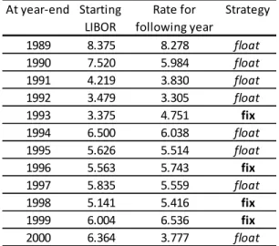
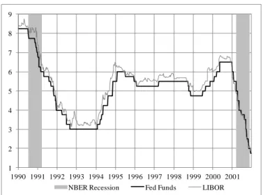
Below, we examine the data for clues based on the above arguments. Over our sample period, the interest rate varied significantly and had several surprises. Figure 4 displays the development of the Fed Funds rate and LIBOR over the sample period, and shows (in Panel b) the direction in which pfix would need to change in a given year for the firm to benefit from changes in the Fed Funds rate the following year. Table VII contains the same information as Figure 4b. This interpretation only considers interest expense in the context of the current thought experiment, and is not a general rule. A firm is classified as Right in a particular year if it had changed its pfix the previous year in the same direction as stated in Table VII, and Wrong otherwise.
5.1. Question 1: Do firms that appear to anticipate rates more often display any advantages over those that don’t?
As noted above, a firm could be Right in one year and Wrong the next. To determine whether a firm was Right more often, we take the average of Right (which is a binary variable) for each firm over 10 years. Firms that were in the 60th percentile or higher of being Right on average are
[23]
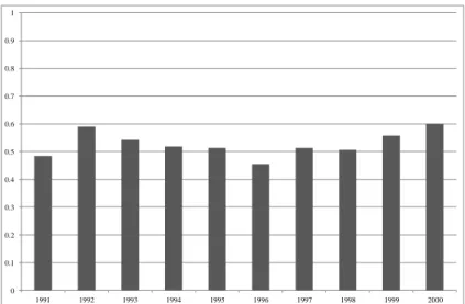
labeled AllRight, and those that were in the 40th percentile or below are the other group. The distribution of the variable AllRight across firms is provided in Figure 5. Similarly, the proportion of firms that were Right in any given year is provided in Figure 6. This proportion is between 40% and 60% in any single year, so that firms were evenly distributed between the two categories although the composition of each group was not the same from year to year.
[Insert Figure 4, Table VII, Figure 5 and Figure 6 here]
We now run a probit regression to check if there is any feature of a firm that would predict that it is more likely to belong to the AllRight group. Resoundingly, none of the characteristics (size, profitability, liquidity, cost management) have a significant coefficient. If we had found any significant association, it might point to an explanation for firms being more often Right (such as informational advantage due to size), or to evidence that those that are more often Right have some performance differences from their counterparts. Such evidence might have been consistent with the extreme assumption in our thought experiment that all firms are speculating, and might also have led us to explore questions of managerial ability. As such, we have found no significant evidence to lead us in this direction. On the other hand, the two potential alternatives we identified above cannot be ruled out. Firms could be speculating but with no sustainable informational advantage, or they are not speculating and in fact choosing pfix based on other considerations, such as those we found in Section 4. There may be other alternatives we have not explored. Next, we consider the year-by-year classification.
5.2. Question 2: Are there differences between Right and Wrong firms year-by-year?
When pfix choices are made on hedging considerations, the classification into Right and Wrong on a year-by-year basis should be effectively artificial, and we would not expect any evidence of differences in performance between the two groups of firms in a given year. To test this argument, we pool all firm-year observations of Right and Wrong, and compare the two groups using t-tests on various measures of their annual change in performance. We find that there are significant differences between Right and Wrong firms.
[Insert Table VIII here]
The results in Table VIII show that in the year following a Right move, firms were better off compared to their Wrong counterparts due to reduced leverage and superior operating
[24]
performance through lower sales, general and administrative expenses. Finally, they had to issue relatively less short-term debt in that year.4 It is difficult to imagine causation from interest rate decisions to any of the above performance measures, more so because the change in return on assets is not significantly different between the two sets of firm-years, but the change in operating cash flow (which does not take into account the interest expense) is better in Right firms.
One possible explanation for this positive relation is that managers may take a view on future developments in the economy and act on them across the activities of the firm, not just in terms of their interest rate choices. There is empirical evidence in support of the idea that managers make operational changes in response to what they view as changes in exposure (Aabo and Simkins, 2005). If some managers also make such changes based on their views on future interest rate changes, we would expect to see the result in Table VIII. However, combined with the result in Section 5.1, the differences between Right and Wrong firms cannot be attributed to skill, but potentially to luck. In other words, it is possible that when managers guess the direction of the economy correctly, they may make coordinated decisions that give them a short-term advantage in their operational performance as well.
While we cannot consider this to be evidence of speculation, we do see results consistent with the possibility that some managers act on their views when they choose their mix of fixed and floating rate debt. We have also seen that, in the case of interest rates, hedging or speculative behavior is too complex to be captured by a simple proxy such as active swaps usage, or even the level of variation in the share of fixed rate debt. The results in this section point to possible further exploration of alternative indicators of speculation based on the correlation over time between operational results and ex post outcomes of financial choices such as changes in pfix. Several caveats have been identified at the beginning of this Section. Other caveats exist. For instance, firms could change their policies over time. Alternatively, they could be acting over a different horizon. To the extent that the data has offered a clue, it supports the existence of at least some behavior consistent with findings such as those in Geczy et al. (2007) or Aabo and Simkins (2005). A fuller consideration of the caveats discussed above, and of the potential for
4
A referee has pointed out that the average LIBOR did not change significantly in some years. In order to check for robustness, we have also carried out this classification exercise in only three years identified as containing significant interest rate surprises: the 1994 and 1998 tightening, and the 2001 easing. The results with respect to operating performance remain similar, though the difference in leverage is no longer significant.
[25]
constructing new indicators of speculation based on the findings in this Section is left to future work.
6. Conclusion
We have studied the proportion of fixed rate debt in firms by using hand-collected data from a specific period of time when this type of data retrieval is informative. Our analysis reconciles some of the mixed results in the literature and extends it by considering a further refinement of data to identify the existence of different hedging motives in firms that vary their interest rate mix to a lesser or greater extent. We also document the nature and striking level of variation in the proportion of fixed rate for individual firms over time.
We also contribute by proposing a further method to identify speculative activity by firms. We have shown how both simple and sophisticated attempts at classifying a particular position as speculative or a hedge could fail when we do not take other operational information into account. We find evidence consistent with Almeida et al. (2011), whereby firms with lower leverage and potential financing constraints are seen to be actively hedging their exposures. While firms with high leverage and more fixed rate debt retain more liquidity, those with lower leverage and more floating rate debt tend to have higher operating cash flows.
Several questions still remain. The fact that the mean across firms of pfix is relatively stable suggests that the demand and supply effects transmitted through the financial intermediary sector are playing a role. This argument is developed in the context of the maturity choice by Greenwood, Hanson and Stein (2010).
We found that Active firms and those that are more often Wrong are not less valuable than their counterparts on average. The implications of this for discriminating between ex-ante and ex-post income smoothing require further study.
The results in this paper are particularly relevant to the two-sided nature of interest rate risk and may not be straightforward to apply to other sources of financial market risk. We have also presented a simple framework that moves towards establishing a benchmark rule for the optimal mix of fixed and floating rate debt. We leave dynamic extensions of the model for future work.
[26]
References
Aabo, T, Simkins, B.J., 2005. Interaction between real options and financial hedging: Fact or fiction in managerial decision-making. Review of Financial Economics 14, 353-369. Acharya, V.V., Almeida, H., Campello, M., 2007. Is cash negative debt? A hedging perspective
on corporate financial policies. Journal of Financial Intermediation 16, 515-554.
Adam, T., Dasgupta, S., Titman, S., 2007. Financial constraints, competition, and hedging in industry equilibrium. The Journal of Finance 62, 2445-2473.
Adam, T.R., Fernando, C.S., 2006. Hedging, speculation, and shareholder value. Journal of Financial Economics 81, 283-309.
Adam, T.R., Nain, A., 2013. Strategic risk management and product market competition. In: Batten, J.A., MacKay, P., Wagner, N. (Eds.), Advances in Financial Risk Management. Palgrave Macmillan.
Allayannis, G., Ihrig, J., Weston, J.P., 2001. Exchange-rate hedging: Financial versus operational strategies. American Economic Review 91, 391-395.
Almeida, H., Campello, M., Weisbach, M.S., 2011. Corporate financial and investment policies when future financing is not frictionless. Journal of Corporate Finance 17, 675-693. Arak, M., Estrella, A., Goodman, L., Silver, A., 1988. Interest rate swaps: An alternative
explanation. Financial Management 17, 12-18.
Aretz, K., Bartram, S. M., 2010. Corporate hedging and shareholder value. Journal of Financial Research 33, 317-371.
Bartram, S. M., 2008. What lies beneath: Foreign exchange ra