Large-scale Medical Image Processing

저작자표시-비영리-변경금지 2.0 대한민국 이용자는 아래의 조건을 따르는 경우에 한하여 자유롭게 l 이 저작물을 복제, 배포, 전송, 전시, 공연 및 방송할 수 있습니다. 다음과 같은 조건을 따라야 합니다: l 귀하는, 이 저작물의 재이용이나 배포의 경우, 이 저작물에 적용된 이용허락조건 을 명확하게 나타내어야 합니다. l 저작권자로부터 별도의 허가를 받으면 이러한 조건들은 적용되지 않습니다. 저작권법에 따른 이용자의 권리는 위의 내용에 의하여 영향을 받지 않습니다. 이것은 이용허락규약(Legal Code)을 이해하기 쉽게 요약한 것입니다. Disclaimer 저작자표시. 귀하는 원저작자를 표시하여야 합니다. 비영리. 귀하는 이 저작물을 영리 목적으로 이용할 수 없습니다. 변경금지. 귀하는 이 저작물을 개작, 변형 또는 가공할 수 없습니다.

Master's Thesis

Large-scale Medical Image Processing

Jisoo Kim

Department of Electrical Engineering

Graduate School of UNIST

2020

Large-scale Medical Image Processing

Jisoo Kim

Department of Electrical Engineering

Abstract

Deep learning based approaches for vision motivated many researchers in Medical Image processing fields due to the powerful performances. Compare to the natural image data, the medical image data set commonly consumes huge memory with complex data structures. In addition, to demonstrate the large scale images for clin-ical purpose such as CT scans or pathologclin-ical image data, it is commonly known to be difficult so that direct application of conventional deep models with typical GPU usage should be considered. For example, in the pathological data which is the image of microscope of human cells to classify tumor cells or not, the size of image slide is far larger than natural high resolution images while the field of view (FOV) that we are interested region is tiny. On the other hand, to handle the large scale of CT data which is using X-ray beams to visualize in-vivo hardness structures, due to the memory limitation of GPU device, the patch-wise method is suppressed to yield high performance and is disturbed to compute faster. Thus, in this paper, we investigate the how data balancing method effectively enhance the deep approach method when there is only unbalanced dataset. Furthermore, we propose the effi-cient memory utilization of multi-gpu method for deep learning with large scale CT images.

Contents

Contents iv

List of Figures vi

List of Tables vii

I. Introduction 1

II. Patch-based data balancing method with pathology images for efficient deep learning 4

2.1 Related work . . . 4

2.2 Methods . . . 5

2.2.1 Heatmap generation for tumor areas . . . 5

2.2.2 Data balancing method . . . 6

2.2.3 Results . . . 7

2.2.4 Classification of cancer metastasis status . . . 7

2.3 Experimental Results . . . 8

2.3.1 Experiment setup . . . 8

2.3.2 Results . . . 8

2.4 Discussion . . . 9

III. Efficient usage of limited GPU memory for Sparse view CT artifacts removing 10 3.1 Related work . . . 10

3.1.1 Sparse view CT artifacts removing . . . 10

3.1.2 Efficient usage of GPU memory . . . 12

3.2 Methods . . . 14

3.2.1 Generating sparse-view CT data . . . 14

3.2.2 Removing sparse-view CT artifacts . . . 15

3.3 Experimental Results . . . 17

3.3.1 Experiment setup . . . 17

3.4 Discussion . . . 19

IV. Conclusion 23

List of Figures

2.1 Whole slide image(WSI) and ground-truth mask of Camelyon17 dataset. [1] . . . 5

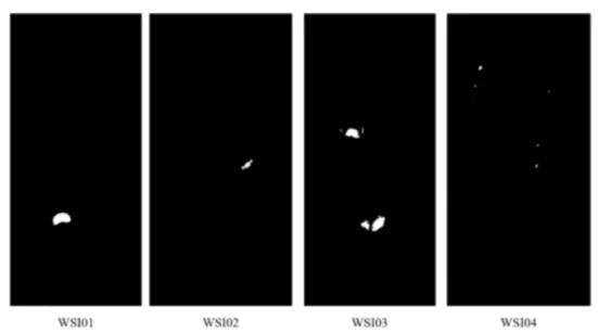
2.2 Tumor areas (white) and normal areas (black) in binary ground-truth masks from 4 different WSIs. . . 6

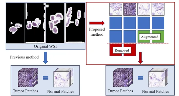
2.3 Proposed data balancing method. . . 7

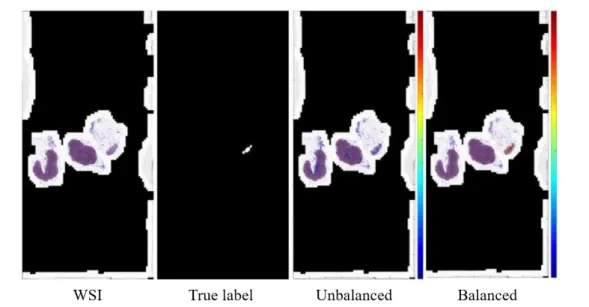
2.4 Results of overlaid probability heat map our proposed data balancing of tumor patch counts. . . 9

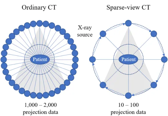
3.1 Data generation of ordinary CT scanner and sparse-view CT scanner. . . 11

3.2 Original CT and Sparse-view CT images . . . 11

3.3 Network training method of data parallel multi-gpu. . . 13

3.4 Multi-gpu communication method of distributed tensorflow [2] . . . 14

3.5 Multi-gpu communication method of horovod [3] . . . 14

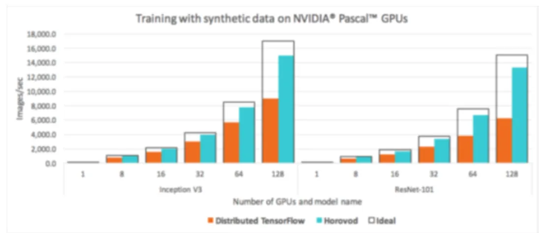
3.6 Performance comparison graph of the number of GPUs between horovod and distributed tensorflow. [3] . . . 15

3.7 Original U-net model [4] . . . 16

3.8 Training process. . . 16

3.9 The result graph of training process at fixed batch size. . . 17

3.10 The result graph of training process at each batch size. . . 19

3.11 The result graph of training process using downsized CT image at each batch size. 20 3.12 The qualitative results of our methods. (a) is sparse view CT image(input), (b),(c),(d),(e) are predicted results of model when batch size set 1, 1-2, 1-4 and 1-2-4. (f) is full view CT image(ground-truth). . . 21

List of Tables

2.1 The number of tumor patches using proposed data balancing method. . . 6

2.2 All 11 features for classification of cancer metastasis. [5]. . . 8

2.3 pN-stage criteria. [1] . . . 8

2.4 Jaccard Index scores our proposed data balancing. . . 9

3.1 The quantitative results of training process at each batch size. . . 19

3.2 The quantitative results of training process using downsized CT image at each batch size. . . 20

CHAPTER

I

Introduction

Pathological data is one of the representative large-scale medical images. Camelyon17 [1] is a challenge that aims to classify cancer stages (pN-stage) through these whole-slide-images(WSI). In digital pathology, classifying cancer stages (pN-stage) through WSI is very important. How-ever, as the automation of pathological image generation accelerates, it is time-consuming to examine ultra-high resolution WSI images in detail and there is a risk of overworking the pathol-ogists and the resultant decrease in examination accuracy. Fine-grained observation of ultra-high resolution WSI and the use of technology to identify and classify metastatic areas have greatly improved accuracy due to a variety of factors, including recent advances in deep learning and public data on breast cancer metastasis such as Camelyon challenges [1]. The winner of Came-lyon 17 [1], Lee at al. [5] used deep learning model resnet101 [6] to detect tumor areas and classify each WSI through a random forest. Finally, they determined the pN-stage based on the classified results. However, there are still many technical challenges, such as the need to use effectively and efficiently large amounts of data, and to deal with different transition imag-ing features of various organs. Therefore, for effective pathological deep learnimag-ing learnimag-ing, we proposed a data balancing technique. Through this, the small sized cancer metastasis area was effectively detected, and the classification result of cancer progression was also derived through the classifier.

Despite the improved performance of finding tumor areas using these data balancing tech-niques, the problem still remained. Still, the pathology image was so intractably large that it

took a long time for the model to learn once. This has been a major obstacle to the develop-ment of models and methods through various experidevelop-ments. Thus, we began to study how to use multiple GPUs at the same time, instead of using one GPU.

The use of multi GPU is natively supported by many deep learning frameworks such as tensorflow [7], keras [8], and pytorch [9], and Uber’s horovod [3] has improved performance by optimizing the use of muti-gpu in tensorflow. They used a method that helped speed up by optimizing the communication speed between the GPU and the CPU and between the GPU and the GPU. Of course, speeding up is important, but there are also downsides. These methods eventually help a lot in large multi-GPU systems, but in reality they do not show a noticeable performance improvement in environments that only use up to four GPUs. Figure 3.6 shows a graph of performance improvements when horovod is applied by Uber and Nvidia. In addition, these methods do not increase the memory of the maximum available GPU. Therefore, rather than using multi-gpu to increase the memory of a physically available GPU, we studied how to use the GPU memory efficiently on a single GPU.

Because large-scale medical images have large image sizes, the available memory limit of the GPU is one of the important considerations in our research. According to Goyal et al. [10], The larger the minibatch size, the faster training speed of the model and the better the performance. And then, Smith et al. [11] investigated the effect of changing batch size when deep learning network is training. If batch size is increased during the training process, their performance can be improved. So we looked forward to improving performance, learning speed, and increasing efficiency, and we studied how to make the mini-batches larger by optimizing the memory of the GPU in a single server or single GPU environment.However, there are some of problems explained earlier in using pathological data, so we decided to use CT data. There are two main reasons for using CT data instead of pathological data. First of all, it is suitable for observing the change according to the batch size because the image size of the CT data is so large that a lot of data cannot be used in a batch. In addition, the problem in CT data is not difficult to train the model compared to the pathology data studied previously, and the result can be intuitively checked. We set our problem to remove noise and artifacts that occur in sparse-view CT images that reduced the projection view in a ordinary CT image. When reconstruction of the sparse-view CT, lattice artifacts are generated throughout the image. Recent studies using deep learning have solved this problem using a U-net [4] based model. [12–14] Following this research flow, we used the method of removing noise and artifacts of sparse-view CT using deep learning model based on U-net.

However, increasing physically usable memory through multi-gpu had physical limitations, so we firstly studied how to use memory efficiently on single GPU. In addition, we conducted a

variety of studies on the benefits of increasing the batch size, which is the main reason for using large amounts of memory. We added batch normalization and sigmoid functions in the basic U-net model and made some minor tweaks. As a result, in the same experimental environment, an minimum of 0.2195 and up to 3.1326 improvements in train PSNR(dB) when only batch size was changed.

According to Goyal et al. [10] and Smith et al.. [11], We conducted a study with the goal that larger minibatches helped learning. However, we are currently conducting all experiments on a single GPU, and plan to study it on a multi GPU in the future. Therefore, through the previous researches, we plan to finally go back to the pathological data and solve the problem of the speed of learning about the huge data that was problematic.

CHAPTER

II

Patch-based data balancing method with

pathology images for efficient deep learning

2.1

Related work

Nowadays, deep learning has been commonly used to solve various problems. In this regard, studies have also been conducted in the pathology area to solve problems using deep learning. [5, 15–17] Pathological data consists of microscopic images of the patient’s lesion tissue, which is very large (200, 000×100, 000 pixels) for the original image. In general, pathologists use this image to locate a patient’s lesion and identify its carcinoma. Figure 2.1 shows the whole slide image (WSI) of the camelyon17 [1] dataset, and the corresponding ground-truth mask.

Camelyon16 [18] was a challenge to find the lesion site on a whole slide image (WSI) of the patient’s breast cancer tissue. In Camelyon16 [18], Liu et al. [16] cut a WSI into a patch of 299×299 and regression it using GoogleNet-v1 [19] to create a heatmap of the cancerous distribution in WSI. Through this, they found the area of cancer in WSI. The next year’s challenge, Camelyon17 [1], was a TNM staging challenge for WSI. TNM staging [20] refers to determining the pN-stage for each WSI, which is divided into five categories: pN0, pN0 (i +), pN1mi, pN1, and pN2. Lee et al. [5], who won first place, performed TNM staging for each WSI through the following process. 1) Extract the region of interest. 2) Regression of WSI to Patch based (256×256) using CNN. 3) Generate probability heatmap using the previous results. 4) Classification using feature vector extraction and random forest classifier.

Figure 2.1: Whole slide image(WSI) and ground-truth mask of Camelyon17 dataset. [1]

2.2

Methods

Lee at al. [5] performed the TNM stage classification through the following process: 1)The probability heat map generation by detecting tumor areas from original whole-slide-image, 2) Extracting 11 feature vectors from the generated probability heat map, 3) Classifying each whole-slide-image based on feature vectors extracted using random forest classifier, 4) Determine pN-stage based on a total of five whole-slide-image classifications per each patient. We have proposed a method to improve performance based on [5]. Since each whole-slide-image has a different tumor shape and size of areas, we scaled the size of this area.

2.2.1 Heatmap generation for tumor areas

We used a deep learning network to find tumor areas of breast cancer. We cut 256×256 patches from whole-slide-image and entered it into the resnet101 model [6], one of the popular deep learning networks. Through this process, the probability of tumor area for each patch comes out. However, the original resnet101 [6] is a model for image classification and their outputs are 1000. So, we modified it that has one output as the probability of tumor area. We created a heat map that represents the probability of a tumor area using all the patches of one whole-slide-image. These heat maps intuitively show the tumor area predicted by the deep learning model.

Figure 2.2: Tumor areas (white) and normal areas (black) in binary ground-truth masks from 4 different WSIs.

2.2.2 Data balancing method

In the process of generating the heatmap, we found that the size of the Tumor area was very different for each whole-slide-image. Figure2.2 shows the four whole-slide-image binary masks of the Camelyon17 [1] dataset. This difference was a major obstacle to deep learning models learning to find tumor areas. Naturally, the typical deep learning model is good at learning what it see often, while not learning what it haven’t seen often. For that reason, previous studies [5,15–17] have trained models by matching the number of tumor patches and normal patches. This method helped to improve the performance, but it was limited to whole-slide-image with large tumor area. Therefore, we not only matched the number of tumor patches and normal patches, but also the size of the tumor area for each whole-slide-image.

We performed data balancing in the tumor area by the following process: 1) In all datasets, measure the number of tumor patches for each whole-slide-image, 2) Average the measured counts, 3) In order to match the number of tumor patches of all whole-slide-image, if more than the average, patch is deleted randomly, if less than the average, increase the number of patches through data augmentation. Using these balanced patches, we matched the number of

Table 2.1: The number of tumor patches using proposed data balancing method.

WSI01 WSI02 WSI03 WSI04

Before 1123 209 1823 84

Figure 2.3: Proposed data balancing method.

tumor patches with the number of normal patches just like the previous methods. Figure2.3is a simplified illustration of the proposed method. For example, as shown in Table2.1, when using a total of four whole-slide-images in the total Camelyon17 [1] dataset, we averaged the different numbers of whole-slide-image patches and made it to have about 810(810 or 811) patches for each whole-slide-image.

2.2.3 Results

2.2.4 Classification of cancer metastasis status

Lee at al. [5] used a random forest classifier to classify each whole-slide-image. First, a total of 11 feature vectors were extracted from the probability heat map generated by whole-slide-image. table2.2[5] shows the criteria for extracting the 11 feature vectors they proposed. Next, to classify whole-slide-image into four categories: negative, micro metastasis, macro metastasis, and isolated tumor cells (itc), they used a random forest classifier. Finally, the final goal of the Camelyon17 [1] challenge, TNM stage classification, is performed using the criteria described in the table2.3 [1]. These criteria were provided by Camelyon17 [1].

Table 2.2: All 11 features for classification of cancer metastasis. [5]. No. Feature description

1 largest tumor’s major axis length

2 largest tumor’s maximum confidence probability 3 largest tumor’s average confidence probability 4 largest tumor’s area

5 average of all tumor’s averaged confidence probability 6 sum of all tumor’s area

7 maximum confidence probability in WSI 8 average of all confidence probability in WSI 9 number of regions in WSI

10 sum of all foreground area in WSI

11 foreground and background area ratio in WSI

Table 2.3: pN-stage criteria. [1] pN0 No micro-metastases or macro-metastases or ITCs found. pN0(i+) Only ITCs found.

pN1mi Micro-metastases found, but no macro-metastases found.

pN1 Metastases found in 1-3 lymph nodes, of which at least one is a macro-metastasis. pN2 Metastases found in 4-9 lymph nodes, of which at least one is a macro-metastasis.

2.3

Experimental Results

2.3.1 Experiment setup

We did not use all the WSIs of camelyon17 [1] for model learning, we chose only four WSIs for our experiments. Each WSI was split into 256×256 patches and entered into resnet101 [6]. Probability heat maps were generated for each WSI by collecting the probabilities of the tumor areas. In the training process, we used the cross entropy function as the loss function, Adam optimizer as the optimizer, and set the experiment with the learning rate 0.0001, batch size 4, and 500 epochs.

Then we trained the WSIs of all camelyon17 [1] train datasets through the model. The random forest classifier was trained using the generated results, and 400 of the total 500 were used as train sets and the remaining 100 as validation sets.

2.3.2 Results

Table2.4shows the change in the Jaccard Index score of the our proposed data balancing on 4 WSIs. In all WSIs, the respective scores rose 139-1759%. In particular, the WSI02, which had a very small tumor area, showed the biggest performance improvement. Figure 2.4 shows the

Figure 2.4: Results of overlaid probability heat map our proposed data balancing of tumor patch counts.

Table 2.4: Jaccard Index scores our proposed data balancing.

WSI01 WSI02 WSI03 WSI04

Before proposed method 0.2869 0.0100 0.2664 0.0227 After proposed method 0.3978 0.1759 0.5627 0.0380 Performance improvement 139% 1759% 211% 167%

probability heat map before and after data balancing of WSI02. In the figure2.4, the balanced results find the tumor area well in red, while the unbalanced results do not find well.

2.4

Discussion

In this paper, we studied the effects that can be obtained by matching the tumor area ratio in each WSI and proposed data balancing methods. The simple method has brought great effects, but the learning process still takes a long time, which makes the experiment time very long. Therefore, we plan to study ways to reduce learning time and make learning more efficient.

CHAPTER

III

Efficient usage of limited GPU memory for

Sparse view CT artifacts removing

3.1

Related work

3.1.1 Sparse view CT artifacts removing

In X RAY CT (computed tomography), reducing the scanning time is one of the most important parts. If the scanning time is shortened, hospitals can reduce the time required per patient, and patients will be less exposed to X RAY, reducing the chance of health problems. Therefore, many researchers aimed to reduce the radiation dose in order to reduce the scanning time. Sparse view CT have been proposed as one of these low-dose CTs. [21–29] Figure3.1shows the differences between the ordinary CT and sparse view CT image on scanning procedures. A ordinary CT has about 1000-2000 projection data and a Sparse-view CT has 10-100 projection data. [30] While sparse view CT can significantly reduce scanning time, certain artifacts are left behind when performing FBP (filtered back projection) reconstruction. Figure 3.2 shows the image of sparse view CT according to the difference between the original image and the number of view.

Before deep learning was commonly used to remove artifacts and noise from low-dose CT, various studies have been conducted in the traditional methods. These methods divided into following three categories: 1) Filtering sinogram before reconstruction. [31–33] 2) Iterative re-construction. [34,35] 3) Post-processing the image after reconstruction. [36–38]

Figure 3.1: Data generation of ordinary CT scanner and sparse-view CT scanner.

First, sinogram filtering is a method to improve the quality of raw data before filtered back projection(FBP). Next, iterative reconstruction is a way to solve the problem repeatedly with information such as the target image prior information. Various priors have been proposed, such as dictionary learning, nonlocal means, and total variation [21,39–44]. However, the two previous approaches had difficulty despite the successful approach. Compared to other natural image data, it is difficult to obtain a large amount of good quality data. In addition, interative reconstruction requires huge computational costs. On the other hand, post-processing the image after reconstruction had the advantage of being independent of projection data, of being directly applied to low-dose CT images, and of being easily applicable to CT workflows. However, it was difficult to apply effectively with traditional image denoising method, because the noise of low-dose CT is not uniform distribution, Therefore, effective methods have been proposed such as K-SVD to low-dose CT [37], and a block-matching 3D algorithm. [45]

However, deep learning is now used in many areas, and most of the methods go beyond the performance of traditional methods. Therefore, some researches have been conducted in this area to solve problems using deep learning. However, as with traditional denoising, general denoising methods using convolution neural network(CNN) had difficulty removing noise and artifacts from low-dose CT effectively. [46–48] The reason for this is that artifacts in low-dose CT are generated entirely, so a CNN with a large receptive field is needed, rather than a general CNN. Therefore, methods based on U-net [4] have been proposed. Jin et al. [13] proposed Deep convolutional neural network for inverse problems in imaging, Han et al. [12] proposed deep residual learning for compressed sensing CT reconstruction via persistent homology analysis. Framing U-Net via deep convolutional framelets as application to sparse-View CT was proposed py Han et al. [14]. Therefore, in this paper, we tried to remove noise and artifacts of sparse view CT after FBP using U-net based model.

3.1.2 Efficient usage of GPU memory

The medical images have a larger image size and complexity than natural images. Based on data from Camelyon17 [1], the pathology data has a size of 200, 000×100, 000. In addition, since it consists of similar but different data, it has a lot of difficulties to use in deep learning. Therefore, training deep learning models using pathological data uses a relatively large amount of memory on the GPU. According to [10], GPU memory size is one of the most important parts of deep learning. Goyal et al. [10] shows that as the minibatch size increases, the learning speed and learning results improve. To increase the minibatch size, we usually need to increase the memory size of the GPU.

Figure 3.3: Network training method of data parallel multi-gpu.

One way to increase the amount of physically available GPU memory is by using multiple GPUs at the same time. There are two main ways to use multi-GPU, one is to parallelize the model, and the other is to parallelize the data. Parallelizing a model means dividing the parts of the model so that they are trained on different GPUs. However, this method has a disadvantage in that it is difficult to apply in the structure where the start and end parts are connected by skip-conection such as U-net [4]. Next, the way to parallelize data is generally: 1) Create a copy of the model. 2) Assign the copied model to each GPU. 3) Calculate loss and gradient on each GPU. 4) Model update according to optimization algorithm using calculated loss and gradient. The figure3.3 is a simplified illustration of the process of using multi-gpu.

Tensorflow [2,7], keras [8], pytorch [9], etc., the deep learning framework used by many people, have supported multi gpu method based on data parallelism. In addition, methods such as Uber’s horovod [3] and Nvidia’s NCCL improve basic algorithms to increase efficiency when using multi gpu, optimizing the communication speed between GPU and CPU, between GPU and GPU, and between GPU server and GPU server. The figure 3.4 shows how the typical distributed tensorflow [2] uses multi-gpu. In basic distributed tensorflow, each worker gets in-formation through parameter server. On the other hand, the ring all reduce [49] method applied by horovod does not use a parameter server, but exchanges information through communica-tion between workers. Figure3.5is a simplified illustration of how ring all reduce works. In this way, they could reduce the delay in the communication process and made the multi gpu more efficient. Figure 3.6 shows the speed difference between a model is applied basic distributed

Figure 3.4: Multi-gpu communication method of distributed tensorflow [2]

Figure 3.5: Multi-gpu communication method of horovod [3]

Tensorflow [2] and a model is applied horovod [3].

As you can see in Figure 3.6, horovod can be very helpful when using a large GPU cloud, but in general, for gpu server, which is used for research purposes, it is not efficient because only 4 gpu can be used at the same time. In addition, the previous methods can greatly help speed optimization when using multi-gpu, but the available memory is still limited. Therefore, in this paper, we studied how to efficiently use the limited gpu memory in a single gpu over the efficient use of the gpu memory in a multi-gpu.

3.2

Methods

3.2.1 Generating sparse-view CT data

Figure 2 shows the differences between the generation method of a ordinary CT and a sparse-view CT. Through following method, we created a sparse-sparse-view CT image from the CT image taken in the usual way. 1) Generates a sinogram by radon transforming a normal CT image. 2) Create the desired views. 3) In the process of reconstruction of the sinogram using iradon, reconstruction only as much as the previously generated view. Figure 3.2 shows the original normal CT image and the sparse view CT image generated.

Figure 3.6: Performance comparison graph of the number of GPUs between horovod and dis-tributed tensorflow. [3]

3.2.2 Removing sparse-view CT artifacts

U-net [4] has been used for image to image methods in various fields such as image recon-struction and segmentation. In addition, studies on removing noise and artifacts from sparse view CT data have been using the proposed models based on U-net [4]. [12–14] Figure3.7shows the original structure of the U-net proposed by Ronneberger et al [4].

Since our ultimate goal was not to end up removing the noise and artifacts of sparse view CT, we focused on studying efficient GPU usage. Therefore, we studied and experimented with methods to achieve optimal performance on a single GPU. In order to compare the results according to the batch size, we added batch normalization in the original U-net [4], and we added sigmoid funcion as the activate function at the end of the model to compare about the results with or without activate funtion. Also, since the original U-net [4] has different inputs and outputs, we added paddings to make them the same size.

We used the sparse view CT image created earlier as a input and the original full view CT image as a ground-truth. The process of training the model was as follows: 1) Preparation: Import the original CT image and sparse view CT image and normalize them to 0-1. 2) Batch generation: Prepare to put the batch size image into the model. 3) Model training: Loss and gradient calculation by comparing the prediction result output from the model with the nor-malized original CT image. 4) Update the model based on the calculated values. 5) Repeat the process 1-4 until all the data is used up. 6) Repeat the process of 1-5 for the set maximum epoch. Figure3.8shows the model training process in this paper.

Figure 3.7: Original U-net model [4]

3.3

Experimental Results

3.3.1 Experiment setup

We set up the following experiment to observe changes in train loss, PSNR, validation loss, and PSNR according to batch size within the limited memory of a single GPU. First of all, we unify the overall experimental setting except the batch size. As an initial batch size for all experiment, we set 1. This value is increased up to our pre-defined batch size on every 5 epoch. For example, when the maximum batch size is 4, it is increased up to 2 from 1 at last 10th epoch and it is again increased up to 4 from 2 at last 5th epoch. In similar way, if the maximum batch size is 32, it is increased repeatedly from last 75 epoch. Since the physical limitation for usage of GPU is only batch size 4, we designed 4 experiment as following: 1) batch size is not increased from 1, 2) from last 10 epoch, increased up to 2, 3) from last 10 epoch, increased up to 4, 4) from last 10 epoch, increased up to 2, then increased up to 4 again at last 5 epoch. Note that the image size in this experiment was cropped from 512× 512 to 128× 128 for handling the as many as images with larger batch size in limited GPU memory.

Before all experiments, rather than changing the batch size during training, we set up another

experiment to see what results would be achieved by increasing the batch size from scratch. In this experiment, we simply trained from start to finish with the batch size fixed at 1, 2, 4, 8, 16, 32, 64. Figure3.9shows the results for this experiment. In this experiment, the best results were obtained when setting batch size to 1. As the batch size increases in each epoch, the iteration count decreases.

All experiments were conducted up to 100 epochs, the learning rate was 0.001, the optimizer was SGD, and loss function was fixed mean absolute error(MAE). We also changed the size of the image using bilinear interpolation to change the image size. The train dataset consists of 4800 images, of which 10%, 480, were used as the validation dataset, and the data order of each epoch shuffled randomly.

In this experiment, we used python 3.7 version, pytorch 1.0.0 version as deep learning frame-work, CUDA version 9.0, Nvidia Xp (pascal) GPU.

3.3.2 Results

In this experiment, we investigate the performance changes by different batch sizes. Fig-ure3.10shows the loss ans PSNR changes among the epoch is increased. In top left figure, the train loss graph, as soon as the batch size is changed, the loss value decreases momentarily. The train PSNR also rises momentarily whenever the batch size changes. If we change the batch size to 2 and then once again to 4 (red line, batch size 1-2-4), the descent will occur every time the batch size changes. Figure3.12shows the qualitative results of our methods. In this figure, (a) is sparse view CT image(input), (b),(c),(d),(e) are predicted results of model when batch size set 1, 1-2, 1-4 and 1-2-4. And (f) is full view CT image as using ground truth. It seems difficult for us to see the difference in performance between predicted images with the naked eye. Table3.1

shows the quantitative results of training process at each batch size. As can be seen in Figure

3.10, the method that moved batch size from 1 to 2 and 2 to 4 showed the biggest performance improvement.

We reduced the size of the image to experiment with increasing the batch size further. By reducing the size of the image by 512×512 to 128×128, we could increase the maximum available batch size from 4 to 64. Figure3.11shows the results of a training process using downsized CT image at each batch size. Looking at the train loss and train psnr on the left, you can see that the performance has risen steeply every 5 epochs. In addition, as the batch size is greatly increased, the performance is also greatly improved. Table3.2shows the quantitative results of training process using downsized CT image at each batch size. In the case of Train psnr, as the batch size was greatly increased, the performance improved by up to 3.14dB.

Figure 3.10: The result graph of training process at each batch size.

3.4

Discussion

In this paper, we studied that the performance improvement can be achieved by simply changing the batch size during the learning process. Increasing the batch size significantly resulted in better performance. However, in this paper, since the original image was made small and experimented, it is difficult to apply in a realistic case. In practice, there is a limit of 4 batch sizes when using the original image. Therefore, in order to apply this study to the original large-scale medical image data, we plan to conduct multi-gpu research through co-work that increases the memory of the gpu.

Table 3.1: The quantitative results of training process at each batch size. Batch size Train loss Train PSNR(dB) Validation loss Validation PSNR(dB)

1 0.00448 44.091 0.00549 42.331

1-2 0.00444 44.044 0.00503 43.181

1-4 0.00439 44.102 0.00482 43.549

Figure 3.11: The result graph of training process using downsized CT image at each batch size.

Table 3.2: The quantitative results of training process using downsized CT image at each batch size.

Batch size Train loss Train PSNR(dB) Validation loss Validation PSNR(dB)

1 0.0048 43.1479 0.0051 42.306 1-2 0.0046 43.3674 0.0047 42.8633 1-4 0.0044 43.6368 0.0046 43.0000 1-8 0.0042 43.9589 0.0046 42.9229 1-16 0.0041 44.2905 0.0047 42.8502 1-32 0.0041 44.9630 0.0047 42.7420 1-64 0.0043 46.2805 0.0047 42.6878

Figure 3.12: The qualitative results of our methods. (a) is sparse view CT image(input), (b),(c),(d),(e) are predicted results of model when batch size set 1, 1-2, 1-4 and 1-2-4. (f) is full view CT image(ground-truth).

CHAPTER

IV

Conclusion

In this study, we investigated efficient methods to deal with large scale medical image in limited resource. Firstly, we proposed data balancing method on the pathological image data. The pathological data shows that the ratio of tumor area to the remaining area is very unbal-anced at about 0.1%, and each WSI has tumor areas of different sizes. Therefore, through our proposed data balancing technique, we matched the proportion of tumor areas in each WSI. As a result, a performance increase of 139%-1759% was achieved.

Since large scale medical images are complex and large, they are dependent on the memory size of the GPU when training deep learning models. we studied the multi GPU method of physically increasing the size of the GPU, but it was not suitable for the general environment. Thus, we studied how to use memory efficiently on a single GPU. Since the pathology data is so large and complex that it is difficult to handle, we used CT data. We made it a problem to remove noise and artifacts from the sparse view CT. We studied the changes in the training process according to batch size. As a result, by changing the batch size under the same conditions, we achived the an minimum of 0.2195 and up to 3.1326 improvements in train PSNR(dB) when only batch size was changed.

We used a large scale image to study on a single GPU. However, we have not yet reached the goal of efficient memory usage on multi GPU, which we ultimately aimed for. Finally, we will study efficient usage the memory of multi GPU to experiment with more complex and huge pathological data than CT data.

References

[1] Oscar Geessink, P´eter B´andi, Geert Litjens, and Jeroen van der Laak, “Camelyon17: Grand challenge on cancer metastasis detection and classification in lymph nodes,” 2017. vi, vii,

1,4,5,6,7,8,12

[2] Mart´ın Abadi, Ashish Agarwal, Paul Barham, Eugene Brevdo, Zhifeng Chen, Craig Citro, Greg S Corrado, Andy Davis, Jeffrey Dean, Matthieu Devin, et al., “Tensorflow: Large-scale machine learning on heterogeneous distributed systems,” arXiv preprint arXiv:1603.04467, 2016. vi,13,14

[3] Alexander Sergeev and Mike Del Balso, “Horovod: fast and easy distributed deep learning in tensorflow,” arXiv preprint arXiv:1802.05799, 2018. vi,2,13,14,15

[4] Olaf Ronneberger, Philipp Fischer, and Thomas Brox, “U-net: Convolutional networks for biomedical image segmentation,” inInternational Conference on Medical image computing

and computer-assisted intervention. Springer, 2015, pp. 234–241. vi,2,12,13,15,16

[5] Byungjae Lee and Kyunghyun Paeng, “A robust and effective approach towards accurate metastasis detection and pn-stage classification in breast cancer,” in International

Con-ference on Medical Image Computing and Computer-Assisted Intervention. Springer, 2018,

REFERENCES

[6] Kaiming He, Xiangyu Zhang, Shaoqing Ren, and Jian Sun, “Deep residual learning for image recognition,” inProceedings of the IEEE conference on computer vision and pattern

recognition, 2016, pp. 770–778. 1,5,8

[7] Mart´ın Abadi, Paul Barham, Jianmin Chen, Zhifeng Chen, Andy Davis, Jeffrey Dean, Matthieu Devin, Sanjay Ghemawat, Geoffrey Irving, Michael Isard, et al., “Tensorflow: A system for large-scale machine learning,” in 12th {USENIX} Symposium on Operating

Systems Design and Implementation ({OSDI} 16), 2016, pp. 265–283. 2,13

[8] Fran¸cois Chollet et al., “Keras,”https://github.com/fchollet/keras, 2015. 2,13

[9] Adam Paszke, Sam Gross, Soumith Chintala, Gregory Chanan, Edward Yang, Zachary DeVito, Zeming Lin, Alban Desmaison, Luca Antiga, and Adam Lerer, “Automatic differ-entiation in pytorch,” 2017. 2,13

[10] Priya Goyal, Piotr Doll´ar, Ross Girshick, Pieter Noordhuis, Lukasz Wesolowski, Aapo Ky-rola, Andrew Tulloch, Yangqing Jia, and Kaiming He, “Accurate, large minibatch sgd: Training imagenet in 1 hour,” arXiv preprint arXiv:1706.02677, 2017. 2,3,12

[11] Samuel L Smith, Pieter-Jan Kindermans, Chris Ying, and Quoc V Le, “Don’t decay the learning rate, increase the batch size,” arXiv preprint arXiv:1711.00489, 2017. 2,3

[12] Yo Seob Han, Jaejun Yoo, and Jong Chul Ye, “Deep residual learning for compressed sens-ing ct reconstruction via persistent homology analysis,” arXiv preprint arXiv:1611.06391, 2016. 2,12,15

[13] Kyong Hwan Jin, Michael T McCann, Emmanuel Froustey, and Michael Unser, “Deep convolutional neural network for inverse problems in imaging,” IEEE Transactions on

Image Processing, vol. 26, no. 9, pp. 4509–4522, 2017. 2,12,15

[14] Yoseob Han and Jong Chul Ye, “Framing u-net via deep convolutional framelets: Ap-plication to sparse-view ct,” IEEE transactions on medical imaging, vol. 37, no. 6, pp. 1418–1429, 2018. 2,12,15

[15] Dayong Wang, Aditya Khosla, Rishab Gargeya, Humayun Irshad, and Andrew H Beck, “Deep learning for identifying metastatic breast cancer,”arXiv preprint arXiv:1606.05718, 2016. 4,6

[16] Yun Liu, Krishna Gadepalli, Mohammad Norouzi, George E Dahl, Timo Kohlberger, Alek-sey Boyko, Subhashini Venugopalan, Aleksei Timofeev, Philip Q Nelson, Greg S Corrado,

REFERENCES

et al., “Detecting cancer metastases on gigapixel pathology images,” arXiv preprint

arXiv:1703.02442, 2017. 4,6

[17] Sanghun Lee, Sangjun Oh, Kyuhyoung Choi, and Sun Woo Kim, “Automatic classification on patient-level breast cancer metastases,” . 4,6

[18] B Ehteshami Bejnordi and Jeroen van der Laak, “Camelyon16: Grand challenge on cancer metastasis detection in lymph nodes,” 2016. 4

[19] Rupesh K Srivastava, Klaus Greff, and J¨urgen Schmidhuber, “Training very deep net-works,” inAdvances in neural information processing systems, 2015, pp. 2377–2385. 4

[20] Leslie H Sobin, Mary K Gospodarowicz, and Christian Wittekind, TNM classification of

malignant tumours, John Wiley & Sons, 2011. 4

[21] Emil Y Sidky and Xiaochuan Pan, “Image reconstruction in circular cone-beam computed tomography by constrained, total-variation minimization,” Physics in Medicine & Biology, vol. 53, no. 17, pp. 4777, 2008. 10,12

[22] Xiaochuan Pan, Emil Y Sidky, and Michael Vannier, “Why do commercial ct scanners still employ traditional, filtered back-projection for image reconstruction?,” Inverse problems, vol. 25, no. 12, pp. 123009, 2009. 10

[23] Junguo Bian, Jeffrey H Siewerdsen, Xiao Han, Emil Y Sidky, Jerry L Prince, Charles A Pelizzari, and Xiaochuan Pan, “Evaluation of sparse-view reconstruction from flat-panel-detector cone-beam ct,” Physics in Medicine & Biology, vol. 55, no. 22, pp. 6575, 2010.

10

[24] Sathish Ramani and Jeffrey A Fessler, “A splitting-based iterative algorithm for accelerated statistical x-ray ct reconstruction,” IEEE transactions on medical imaging, vol. 31, no. 3, pp. 677–688, 2011. 10

[25] Yang Lu, Jun Zhao, and Ge Wang, “Few-view image reconstruction with dual dictionaries,”

Physics in Medicine & Biology, vol. 57, no. 1, pp. 173, 2011. 10

[26] Kyungsang Kim, Jong Chul Ye, William Worstell, Jinsong Ouyang, Yothin Rakvongthai, Georges El Fakhri, and Quanzheng Li, “Sparse-view spectral ct reconstruction using spec-tral patch-based low-rank penalty,” IEEE transactions on medical imaging, vol. 34, no. 3, pp. 748–760, 2014. 10

REFERENCES

[27] Timothy P Szczykutowicz and Guang-Hong Chen, “Dual energy ct using slow kvp switch-ing acquisition and prior image constrained compressed sensswitch-ing,” Physics in Medicine &

Biology, vol. 55, no. 21, pp. 6411, 2010. 10

[28] Sajid Abbas, Taewon Lee, Sukyoung Shin, Rena Lee, and Seungryong Cho, “Effects of sparse sampling schemes on image quality in low-dose ct,” Medical physics, vol. 40, no. 11, pp. 111915, 2013. 10

[29] Taewon Lee, Changwoo Lee, Jongduk Baek, and Seungryong Cho, “Moving beam-blocker-based low-dose cone-beam ct,” IEEE Transactions on Nuclear Science, vol. 63, no. 5, pp. 2540–2549, 2016. 10

[30] Hiroyuki Kudo, Taizo Suzuki, and Essam A Rashed, “Image reconstruction for sparse-view ct and interior ct—introduction to compressed sensing and differentiated backprojection,”

Quantitative imaging in medicine and surgery, vol. 3, no. 3, pp. 147, 2013. 10

[31] Jing Wang, Hongbing Lu, Tianfang Li, and Zhengrong Liang, “Sinogram noise reduction for low-dose ct by statistics-based nonlinear filters,” inMedical Imaging 2005: Image

Pro-cessing. International Society for Optics and Photonics, 2005, vol. 5747, pp. 2058–2066.

10

[32] Jing Wang, Tianfang Li, Hongbing Lu, and Zhengrong Liang, “Penalized weighted least-squares approach to sinogram noise reduction and image reconstruction for low-dose x-ray computed tomography,” IEEE transactions on medical imaging, vol. 25, no. 10, pp. 1272– 1283, 2006. 10

[33] Armando Manduca, Lifeng Yu, Joshua D Trzasko, Natalia Khaylova, James M Kofler, Cynthia M McCollough, and Joel G Fletcher, “Projection space denoising with bilateral filtering and ct noise modeling for dose reduction in ct,” Medical physics, vol. 36, no. 11, pp. 4911–4919, 2009. 10

[34] Marcel Beister, Daniel Kolditz, and Willi A Kalender, “Iterative reconstruction methods in x-ray ct,” Physica medica, vol. 28, no. 2, pp. 94–108, 2012. 10

[35] Amy K Hara, Robert G Paden, Alvin C Silva, Jennifer L Kujak, Holly J Lawder, and William Pavlicek, “Iterative reconstruction technique for reducing body radiation dose at ct: feasibility study,” American Journal of Roentgenology, vol. 193, no. 3, pp. 764–771, 2009. 10

REFERENCES

[36] P Fumene Feruglio, Claudio Vinegoni, J Gros, A Sbarbati, and R Weissleder, “Block matching 3d random noise filtering for absorption optical projection tomography,” Physics

in Medicine & Biology, vol. 55, no. 18, pp. 5401, 2010. 10

[37] Yang Chen, Xindao Yin, Luyao Shi, Huazhong Shu, Limin Luo, Jean-Louis Coatrieux, and Christine Toumoulin, “Improving abdomen tumor low-dose ct images using a fast dictionary learning based processing,” Physics in Medicine & Biology, vol. 58, no. 16, pp. 5803, 2013. 10,12

[38] Jianhua Ma, Jing Huang, Qianjin Feng, Hua Zhang, Hongbing Lu, Zhengrong Liang, and Wufan Chen, “Low-dose computed tomography image restoration using previous normal-dose scan,” Medical physics, vol. 38, no. 10, pp. 5713–5731, 2011. 10

[39] Yi Zhang, Yan Wang, Weihua Zhang, Feng Lin, Yifei Pu, and Jiliu Zhou, “Statistical iterative reconstruction using adaptive fractional order regularization,” Biomedical optics

express, vol. 7, no. 3, pp. 1015–1029, 2016. 12

[40] Yi Zhang, Weihua Zhang, Yinjie Lei, and Jiliu Zhou, “Few-view image reconstruction with fractional-order total variation,” JOSA A, vol. 31, no. 5, pp. 981–995, 2014. 12

[41] Yi Zhang, Wei-Hua Zhang, Hu Chen, Meng-Long Yang, Tai-Yong Li, and Ji-Liu Zhou, “Few-view image reconstruction combining total variation and a high-order norm,”

Inter-national Journal of Imaging Systems and Technology, vol. 23, no. 3, pp. 249–255, 2013.

12

[42] Jianhua Ma, Hua Zhang, Yang Gao, Jing Huang, Zhengrong Liang, Qianjing Feng, and Wufan Chen, “Iterative image reconstruction for cerebral perfusion ct using a pre-contrast scan induced edge-preserving prior,” Physics in Medicine & Biology, vol. 57, no. 22, pp. 7519, 2012. 12

[43] Yang Chen, Zhou Yang, Yining Hu, Guanyu Yang, Yongcheng Zhu, Yinsheng Li, Wufan Chen, Christine Toumoulin, et al., “Thoracic low-dose ct image processing using an artifact suppressed large-scale nonlocal means,” Physics in medicine & biology, vol. 57, no. 9, pp. 2667, 2012. 12

[44] Qiong Xu, Hengyong Yu, Xuanqin Mou, Lei Zhang, Jiang Hsieh, and Ge Wang, “Low-dose x-ray ct reconstruction via dictionary learning,” IEEE transactions on medical imaging, vol. 31, no. 9, pp. 1682–1697, 2012. 12

REFERENCES

[45] Ke Sheng, Shuiping Gou, Jiaolong Wu, and Sharon X Qi, “Denoised and texture enhanced mvct to improve soft tissue conspicuity,” Medical physics, vol. 41, no. 10, pp. 101916, 2014.

12

[46] Yunjin Chen, Wei Yu, and Thomas Pock, “On learning optimized reaction diffusion pro-cesses for effective image restoration,” inProceedings of the IEEE conference on computer

vision and pattern recognition, 2015, pp. 5261–5269. 12

[47] Xiaojiao Mao, Chunhua Shen, and Yu-Bin Yang, “Image restoration using very deep convolutional encoder-decoder networks with symmetric skip connections,” inAdvances in

neural information processing systems, 2016, pp. 2802–2810. 12

[48] Junyuan Xie, Linli Xu, and Enhong Chen, “Image denoising and inpainting with deep neural networks,” in Advances in neural information processing systems, 2012, pp. 341– 349. 12

[49] Pitch Patarasuk and Xin Yuan, “Bandwidth optimal all-reduce algorithms for clusters of workstations,” Journal of Parallel and Distributed Computing, vol. 69, no. 2, pp. 117–124, 2009. 13

Acknowledgement

I cannot believed that it has been already 2 years since i study for master degree. Without so many people around me, this thesis may not have been completed. First of all, I would like to thank to supervisor Professor Se Young Chun for his guidance and teaching for overall of my study and research. If he did not offer me as a master students with this research, i may not achieve this great works and experiences. I also want to express my sincere thanks to my defense committee members: Professor Seung-Joon Yang, for providing the story line comments and encouraging me to understand the level, and Professor Jae-Young Sim for his comments about experimental results description. I would also like to acknowledge lab mates: Hanvit Kim, Thanh Quoc Phan, Magauiya Zhussip, Shakarim Soltanayev, Dong Won Park, Kwan Young Kim, Won Jae Hong, Dong Un Kang, Yong Hyeok Seo. Lastly, I would like to give my very special thanks to my family for always believing in me, especially my parents, who always encouraged me whenever I was down.