This is a repository copy of
Multi-input and dataset-invariant adversarial learning (MDAL)
for left and right-ventricular coverage estimation in cardiac MRI
.
White Rose Research Online URL for this paper:
http://eprints.whiterose.ac.uk/145286/
Version: Accepted Version
Proceedings Paper:
Zhang, L, Pereañez, M, Piechnik, SK et al. (3 more authors) (2018) Multi-input and
dataset-invariant adversarial learning (MDAL) for left and right-ventricular coverage
estimation in cardiac MRI. In: Lecture Notes in Computer Science. 21st International
Conference on Medical Image Computing and Computer-Assisted Intervention - MICCAI
2018, 16-20 Sep 2018, Granada, Spain,. Springer Verlag , pp. 481-489. ISBN
9783030009335
https://doi.org/10.1007/978-3-030-00934-2_54
© Springer Nature Switzerland AG 2018. This is an author produced version of a
conference paper published in Lecture Notes in Computer Science. Uploaded in
accordance with the publisher's self-archiving policy.
[email protected] https://eprints.whiterose.ac.uk/
Reuse
Items deposited in White Rose Research Online are protected by copyright, with all rights reserved unless indicated otherwise. They may be downloaded and/or printed for private study, or other acts as permitted by national copyright laws. The publisher or other rights holders may allow further reproduction and re-use of the full text version. This is indicated by the licence information on the White Rose Research Online record for the item.
Takedown
If you consider content in White Rose Research Online to be in breach of UK law, please notify us by
Learning (MDAL) for Left and Right-Ventricular
Coverage Estimation in Cardiac MRI
Le Zhang1, Marco Perea˜nez1, Stefan K. Piechnik2,
Stefan Neubauer2, Steffen E. Petersen3, Alejandro F. Frangi1
1
Centre for Computational Imaging and Simulation Technologies in Biomedicine, Department of Electronic and Electrical Engineering, University of Sheffield, UK.
2
Oxford Center for Clinical Magnetic Resonance Research (OCMR), Division of Cardiovascular Medicine, University of Oxford, John Radcliffe Hospital, UK.
3
Cardiovascular Medicine at the William Harvey Research Institute, Queen Mary University of London and Barts Heart Center, Barts Health NHS Trust, UK.
Abstract. Cardiac functional parameters, such as, the Ejection Frac-tion (EF) and Cardiac Output (CO) of both ventricles, are most imme-diate indicators of normal/abnormal cardiac function. To compute these parameters, accurate measurement of ventricular volumes at end-diastole (ED) and end-systole (ES) are required. Accurate volume measurements depend on the correct identification of basal and apical slices in cardiac magnetic resonance (CMR) sequences that provide full coverage of both left (LV) and right (RV) ventricles. This paper proposes a novel adver-sarial learning (AL) approach based on convolutional neural networks (CNN) that detects and localizes the basal/apical slices in an image volume independently of image-acquisition parameters, such as, imaging device, magnetic field strength, variations in protocol execution, etc. The proposed model is trained on multiple cohorts of different provenance, and learns image features from different MRI viewing planes to learn the appearance and predict the position of the basal and apical planes. To the best of our knowledge, this is the first work tackling the fully au-tomatic detection and position regression of basal/apical slices in CMR volumes in a dataset-invariant manner. We achieve this by maximizing the ability of a CNN to regress the position of basal/apical slices within a single dataset, while minimizing the ability of a classifier to discriminate image features between different data sources. Our results show superior performance over state-of-the-art methods.
Keywords: Deep Learning·Dataset Invariance·Adversarial Learning ·Ventricular Coverage Assessment·MRI.
1
Introduction
To obtain accurate and reliable volume and functional parameter measurements in CMR imaging studies, recognizing basal and apical slices for both ventricles is crucial. Unfortunately, current practice to detect basal/or apical slice positions is still carried out by visual inspection of experts on the image. This practice is costly, subjective, error prone, and time consuming [1]. Although significant
2
progress [14] has been made in automatic assessment of full LV coverage in cardiac MRI, to accurately measure volumes and functional parameters for both ventricles where the basal/apical slices are missing, methods to estimate the position of the missing slices are required [10]. Such methods would be critical to prompt the intervention of experts to correct problems in data measurements, or to trigger algorithms that can cope with missing data by, for instance, imputation [5] through image synthesis, or shape based extrapolation. This paves the way to “quality-aware image analysis” [13]. To the best of our knowledge, previous work regarding image quality control has focused solely on coverage detection of the LV, but not on missing slice position estimation.
In medical image analysis, it is sometimes convenient or necessary to infer an image in one modality from another for image quality assessment purposes. One major challenge of basal/apical slice estimation for CMR comes from differences between data sources, which are tissue appearance and/or spatial resolution of images sourced from different physical acquisition principles or parameters. Such differences make it difficult to generalize algorithms trained on specific datasets to other data sources. This is problematic not only when the source and target datasets are different, but more so, when the target dataset contains no labels. In all such scenarios, it is highly desirable to learn a discriminative classifier or other predictor in the presence of a shift between training and test distributions, which is called dataset invariance. The general approach of achieving dataset adaptation has been explored under many facets. Among the existing cross-dataset learning works, cross-dataset adaptation has been adopted for re-identification hoping labeled data from a source dataset can provide transferable identity-discriminative information for a target dataset. [7] explored the possibility of generating multimodal images from single-modality imagery. [8] [9] employed multi-task metric learning models to benefit the target task. However, these works are focused mainly on linear assumptions.
In this paper, we focus on the non-linear representations and analysis of short-axis (SA) and long-axis (LA) cine MRI for the detection and regression of the basal and apical slices of both ventricles in CMR volumes. To deal with the problem where there is no labeled data for a target dataset, and one hopes to transfer knowledge from a model trained on sufficient labeled data of a source dataset sharing the same feature space, but with a different marginal distribu-tion we present these contribudistribu-tions: 1) We present a unified model (MDAL) for any cross-dataset basal/apical slice estimation problem in CMR volumes; 2) We integrate adversarial feature learning by building an end-to-end architecture of CNNs and transferring non-linear representations from a labeled source dataset to a target dataset where labels are non-existent. Our deep architecture effec-tively improves the adaptability of learning with data of different databases; 3) A multi-view image extension of the adversarial learning model is proposed and exploited. By making use of multi-view images acquired from short- and long-axis views, one can further improve and constrain the basal/apical slice position. We evaluate our method on three datasets and compare with state-of-the-art methods. Experimental results show the superior performance of our method compared to other approaches.
2
Methodology
2.1 Problem Formulation
The cross-dataset localization of basal or apical slices can be formulated as two tasks: (i) Dataset Invariance: given a set of 3D images Xs = [Xs
1, ...,XsN] ∈
Rm×n×zs×Ns of modality M
s in the source dataset, and Xt = [Xt1, ...,X t N] ∈
Rm×n×zt×Nt of modalityMt in the target dataset.m, nare the dimensions of
axial view of the image, and zs and zt denote the size of images along the
z-axis, whileNsandNtare the number of volumes in source and target datasets,
respectively. Our goal is to build mappings between the source (training-time) and the target (test-time) datasets, that reduce the difference between the source and target data distributions; (ii)Multi-view Slice Regression:In this task, slice localization performance is enhanced by using multiple image stacks, e.g. SA and LA stacks, into a single regression task. Let Xs ={xs
i, rsi}Z s i=1 and Y s = {ys i, ris}Z s
i=1 be a labeled 3D CMR volume from source modality Ms in
short-and long-axis, respectively, short-andxs
b,xsa, andysb,ysa be the short-axis slices, and
long-axis image patches of the basal and apical views; let Xt = {xt i}Z t i=1 and Yt ={yt i}Z t
i=1 represent an unlabeled sample from the target dataset in
short-and long-axis, i represents the ith slice and Z is the total number of CMR
slices. Our goal is to learn the discriminative features fromxs
b,xsa, andysb,ysa to
localize the basal and apical slices in two axes for CMR volumes in the target dataset1. We use the labeled UK Biobank (UKBB) [11] cardiac MRI data cohort
together with the MESA2 and DETERMINE3 datasets, and apply our method
to cross-dataset basal and apical slice regression tasks.
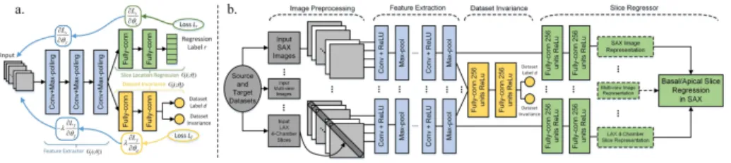
Fig. 1.a:Schematic of our dataset-invariant adversarial network;b:System overview of our proposed dataset-invariant adversarial model with multi-view input channels for bi-ventricular coverage estimation in cardiac MRI. Each channel contains three conv layers, three max-pooling layers and two fully-connected layers. Additional dataset invariance net (yellow) includes two fully-connected layers. Kernel numbers in each conv layer are 16, 16 and 64 with sizes of 7×7, 13×13 and 10×10, respectively; filter
sizes in each max-pooling layer are 2×2, 3×3 and 2×2 with stride 2.
1
Notation: Matrices and 3D images are written in bold uppercase (e.g., image X, Y), vectors and vectorized 2D images in bold lowercase (e.g., slicex,y) and scalars in lowercase (e.g., slice position labelr).
2
http://www.cardiacatlas.org/studies/mesa/
3
4
2.2 Multi-Input and Dataset-Invariant Adversarial Learning
Inspired by Adversarial Learning (AL)[6] and Dataset Adaptation (DA)[12] for cross-dataset transfer, we propose a Dataset-Invariant Adversarial Learn-ing model, which extends the DA formulation into a AL strategy, and performs them jointly in a unified framework. We propose multi-view adversarial learning by creating multiple input channels (MC) from images which are re-sampled to the same spatial grid and visualize the same anatomy. An overview of our method is depicted in Fig. 1. Given two sets of slices{xs
i}Ni=1,{ysi}Ni=1with slice
position labels {rs
i}Ni=1 for training, to learn a model that can generalize well
from one dataset to another, and is used both during training and test time to regress the basal/apical slice position, we optimize this objective in stages: 1) we optimize the label regression loss
Li r=Lr(Gsigm(Gconv(xs,ys;θf);θr), ri) =X i kri−Gsigm(Gconv(xs,ys;θf);θr), ri)k22+ 1 2 kθfk22+kθrk22 , (1)
whereθf is the representation parameter of the neural network feature extractor,
which corresponds to the feature extraction layers. θr is the regression
param-eter of the slice regression net, which corresponds to the regression layers. ri
denotes the ith slice position label. θ
f and θr are trained for the ith image by
using the labeled source data{Xsi,rsi}N
s
i=1 and{Y s i,rsi}N
s
i=1. 2) Since dataset
ad-versarial learning satisfies a dataset adaptation mechanism, we minimize source and target representation distances through alternating minimax between two loss functions: one is the dataset discriminator loss
Li
d=Ld(Gdisc(Gconv(xs,ys,xt,yt;θf);θd), di)
=−X
i
1[od=di] log(Gdisc(Gconv(xs,ys,xt,yt;θf);θd), di), (2)
which classifies whether an image is drawn from the source or the target dataset.
odindicates the output of the dataset classifier for theithimage,θdis the
param-eter used for the computation of the dataset prediction output of the network, which corresponds to the dataset invariance layers;di denotes the dataset that
the example slicei is drawn from. The other is the source and target mapping invariant loss Li f =Lf(Gconf(Gconv(xs,ys,xt,yt;θf);θd), di) =−X d 1
Dlog(Gconf(Gconv(xs,ys,xt,yt;θf);θd), di),
(3) which is optimized with a constrained adversarial objective by computing the cross entropy between the output predicted dataset labels, and a uniform distri-bution over dataset labels.D indicates the number of input channels. Our full method then optimizes the joint loss function
E(θf, θr, θd) =Lr(Gsigm(Gconv(xs,ys;θf);θr), r)
+λLf(Gconf(Gconv(xs,ys,xt,yt;θf);θd), d),
(4) where hyperparameter λ determines how strongly the dataset invariance influ-ences the optimization; Gconv(·) is a convolution layer function that maps an
example into a new representation;Gsigm(·) is a label prediction layer function;
2.3 Optimization
Similar to classical CNN learning methods, we propose to tackle the optimization problem with the stochastic gradient procedure, in which updates are made in the opposite direction of the gradient of Equation (4) to minimize parameters, and in the direction of the gradient to maximize other parameters [4]. We optimize the objective in the following stages.
Optimizing the Label Regressor: In adversarial adaptive methods, the main goal is to regularize the learning of the source and target mappings, so as to minimize the distance between the empirical source and target mapping distributions. If so then the source regression model can be directly applied to the target representations, eliminating the need to learn a separate target regressor. Training the neural network then leads to this optimization problem on the source dataset:
arg min θf,θr { 1 Ns Ns X i=1 Li r(Gsigm(Gconv(xs,ys;θf);θr), ri)}. (5)
Optimizing for Dataset Invariance:This optimization corresponds to the true minimax objective (Ld and Lf) for the dataset classifier parameters and
the dataset invariant representation. The two losses stand in direct opposition to one another: learning a fully dataset invariant representation means the dataset classifier must do poorly, and learning an effective dataset classifier means that the representation is not dataset invariant. Rather than globally optimizing θd
andθf, we instead perform iterative updates for these two objectives given the
fixed parameters from the previous iteration: arg min θd {−1 N N X i=1 Li d(Gdisc(Gconv(xs,ys,xt,yt;θf);θd), di)}, (6) arg max θf {−1 N N X i=1 Li f(Gconf(Gconv(xs,ys,xt,yt;θf);θd), di)}, (7)
whereN =Ns+Ntbeing the total number of samples. These losses are readily
implemented in standard deep learning frameworks, and after setting learning rates properly so Equation (6) only updatesθdand (7) only updatesθf, the
up-dates can be performed via standard backpropagation. Together, these upup-dates ensure that we learn a representation that is dataset invariant.
2.4 Detection and Regression for Basal/Apical Slice Position
We denote ˆHt, ˆGtas extracted query features, and ˆHs, ˆGsas extracted basal/apical
slice representations from SAX and LAX, respectively. In order to regress basal and apical slices according to query features, we compute the dissimilarity ma-trixδi,j based on ˆHt, ˆGt and ˆHs, ˆGs using the volume’s inter-slice distance as:
δi,j( ˆHt,Hˆs,Gˆt,Gˆs) = q ( ˆHi t−Hˆ j s) 2 + ( ˆGi t−Gˆ j s) 2
. Then, ranking can be carried out based on the ascending order of each row of the dissimilarity distance,i.e., the lower the entry valueδi,j is, the closer the basal/apical slice and the query
6
3
Experiments and Analysis
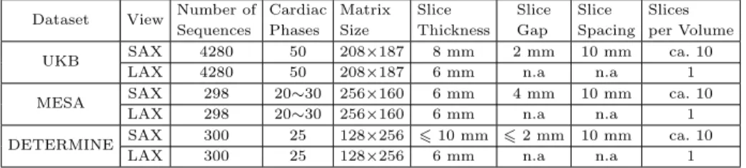
Data specifications:Quality-scored CMR data is available for circa 5,000 vol-unteers of the UK Biobank imaging (UKBB) resource. Following visual inspec-tion, manual annotation for SAX images was carried out with a simple 3-grade quality score [2]. 4,280 sequences correspond to quality score 1 for both ventri-cles, these had full coverage of the heart from base to apex and were the source datasets to construct the ground-truth classes for our experiments. Note that having full coverage should not be confused with having the top/bottom slices corresponding exactly to base/apex. Basal slices including the left ventricular outflow tract, pulmonary valve and right atrium, and apical slices with a visi-ble ventricular cavity were labeled manually. The distance between the actual location of the basal/apical slice to other slices in the volume were used as train-ing labels for the regression. We validated the proposed MDAL on three target datasets: UKBB, DETERMINE and MESA (protocols of the three datasets are shown in Table. 1). To prevent over-fitting due to insufficient target data, and to improve the detection rate of our algorithm, we employ data augmentation techniques to artificially enlarge the target datasets. For this purpose we chose a set of realistic rotations, scaling factors, and corresponding mirror images, and applied them to the MRI images. The set of rotations chosen were −45◦ and 45◦, and the scaling factors 0.75 and 1.25. This increased the number of training samples by a factor of eight. After data augmentation, we had 2400, and 2384 sequences for DETERMINE and MESA datasets, respectively. For evaluating of multi-view models, we defined two input channels, one for SAX images, and another for LAX (4-chamber) from the UKBB, MESA and DETERMINE. The LAX image information was extracted by collecting pixels values along the in-tersecting line between the 4-chamber view plane and corresponding short-axis plane over the cardiac cycle. We extracted 4 pixels above and below the two plane intersection. We embedded the constructed profile within a square image with zeros everywhere except the profile diagonal (see Fig. 1b bottom channel). Table 1. Cardiovascular magnetic resonance protocols for UKBB, MESA and DE-TERMINE Datasets.
Dataset View Number of Sequences Cardiac Phases Matrix Size Slice Thickness Slice Gap Slice Spacing Slices per Volume UKB SAX 4280 50 208×187 8 mm 2 mm 10 mm ca. 10
LAX 4280 50 208×187 6 mm n.a n.a 1 MESA SAX 298 20∼30 256×160 6 mm 4 mm 10 mm ca. 10
LAX 298 20∼30 256×160 6 mm n.a n.a 1 DETERMINE SAX 300 25 128×256 610 mm 62 mm 10 mm ca. 10
LAX 300 25 128×256 6 mm n.a n.a 1
Experimental set-up:The architecture of our proposed method is shown in Fig. 1. To maximize the number of training samples from all datasets, while preventing biased learning of image features from a particular dataset and given that the number of samples from the UKBB is at least an order of magnitude larger than from MESA or DETERMINE, we augmented both the MESA and DETERMINE datasets, to match the resulting number of samples from the UKBB. This way our dataset classification task will not over-fit to anyone
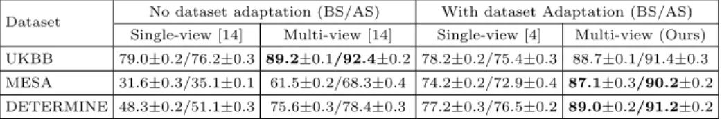
sam-Table 2.The comparison of basal/apical slice detection accuracy (Mean±standard
de-viation) (%) between adaptation and non-adaptation methods, each with single (SAX)-and multi-view inputs (BS/AS indicate basal/apical slice detection accuracy). Best re-sults are highlighted in bold.
Dataset No dataset adaptation (BS/AS) With dataset Adaptation (BS/AS) Single-view [14] Multi-view [14] Single-view [4] Multi-view (Ours) UKBB 79.0±0.2/76.2±0.3 89.2±0.1/92.4±0.2 78.2±0.2/75.4±0.3 88.7±0.1/91.4±0.3 MESA 31.6±0.3/35.1±0.1 61.5±0.2/68.3±0.4 74.2±0.2/72.9±0.4 87.1±0.3/90.2±0.2 DETERMINE 48.3±0.2/51.1±0.3 75.6±0.3/78.4±0.3 77.2±0.3/76.5±0.2 89.0±0.2/91.2±0.2
Table 3.Regression error comparison between adaptation and non-adaptation meth-ods, each with single (SAX)- and multi-view inputs for cardiac SAX slice posi-tion regression in terms of MAE (Mean ±standard deviation)(mm)(BS/AS indicate
basal/apical slice regression errors). Best results are highlighted in bold.
Dataset No dataset adaptation (BS/AS) With dataset adaptation (BS/AS) Single-view [14] Multi-view [14] Single-view [4] Multi-view (Ours) UKBB 4.32±1.6/5.73±1.9 3.42±1.1/3.98±1.7 5.13±2.1/6.33±2.3 3.64±1.9/4.02±2.0 MESA 7.78±2.0/8.34±2.4 6.47±1.7/6.83±1.4 4.81±1.0/5.73±1.5 3.98±1.1/4.07±1.3 DETERMINE 6.43±1.9/6.81±2.0 6.01±1.3/6.17±1.4 4.73±1.6/4.81±1.3 4.24±1.0/4.45±1.3
ple. Our MDAL method processes images with small blocks (120×120), which are crop-centered on the images to extract specific regions of interest. The exper-iments here reported were conducted using the ConvNet library [3] on an Intel Xeon E5-1620 v3 @3.50GHz machine running Windows 10 with 32GB RAM and Nvidia Quadro K620 GPU. We optimize the network using a learning rateµof 0.001 and set the hyper-parameter parameterλto be 0.01, respectively. To eval-uate the detection process, we measure classification accuracy, and to evaleval-uate the regression error between the predicted position and the ground truth, we use the Mean Absolute Error (MAE).
Results:We evaluate the performance of the multi-view basal/apical slice detection and regression tasks with and without dataset invariance (adaptation vs non-adaptation), by transferring object regressors from the UKBB to MESA and DETERMINE. To evaluate performance on MESA and DETERMINE, we manually generated annotations as follows: we checked one slice above and below the detected basal slice to confirm the slice is the basal and record true or false, ditto for apex. We chose the CNN architecture in [14] for single- and multi-view metrics with non-adaptation, and the GTSRB architecture in [4] for single-view adaption method. Table 2 shows the detection accuracy for basal/apical slice of the adaptation and non-adaptation from single and multi-view. For both test datasets, the best improvements are the result of combining both of these fea-tures. For MESA the detection accuracy was increased by 64%, and for DETER-MINE best improvements are of 44% (right-most column). Table 3 shows the average regression errors of slice locations in millimeter (mm). Even without us-ing the multi-input channels, our dataset invariance framework is able to reduce the slice localization error to less than half the average slice spacing found on our test datasets, i.e., <5mm. With multi-view we reduced the localization errors to 4.24 and 4.45mm on average for both basal/apical slices. All the experiences are significantly different atp <0.05.
8
4
Conclusion
In this paper, we have proposed a Multi-Input and Dataset-Invariant Adversarial Learning (MDAL) framework capable of learning a common image representa-tion, and using it to detect and localize basal and apical CMR slices, we achieve this by: first, using a Dataset-Invariant Adversarial Learning (DIAL) model to fit the joint distribution over the images from different datasets with a minimax game. Second, extending the DIAL model to handle multiple view input sce-narios thereby obtaining better results for Left and Right-Ventricular coverage estimation in Cardiac MRI. And third, by introducing a regressor network able to predict the location of basal/apical slices. We evaluated our framework on two large datasets MESA and DETERMINE and found that our approach signifi-cantly outperforms state-of-the-art non-dataset-adaptive and single-input meth-ods. Finally, Our MDAL framework can be easily generalized to any anatomical structure or image modality.
References
1. Attili, A.K., Schuster, A., Nagel, E., Reiber, J.H., van der Geest, R.J.: Quan-tification in Cardiac MRI: Advances in Image Acquisition and Processing. Int J Cardiovasc Imaging 26(1), 27–40 (2010)
2. Carapella, V., et al.: Towards the semantic enrichment of free-text annotation of image quality assessment for UK Biobank cardiac Cine MRI scans. In: Deep Learning and Data Labeling for Medical Applications, pp. 238–248. Springer (2016) 3. Demyanov, S.: ConvNet library for Matlab [Online]. https://github.com/
sdemyanov/ConvNet, accessed 15 Oct. 2017
4. Ganin, Y., Ustinova, E., Ajakan, H., Germain, P., et al.: Domain-Adversarial Train-ing of Neural Networks. J. Mach. Learn. Res. 17(1), 2096–2030 (2016)
5. Garc´ıa-Laencina, P.J., Sancho-G´omez, J.L., Figueiras-Vidal, A.R.: Pattern classi-fication with missing data: a review. Neural Comput Appl 19(2), 263–282 (2010) 6. Goodfellow, I., Pouget-Abadie, J., Mirza, M., Xu, B., Warde-Farley, D., et al.:
Generative adversarial nets. In: Adv Neural Inf Process Syst. pp. 2672–2680 (2014) 7. Huang, Y., Shao, L., Frangi, A.F.: Simultaneous super-resolution and cross-modality synthesis of 3D medical images using weakly-supervised joint convolu-tional sparse coding. IEEE Conference on CVPR pp. 6070–6079 (2017)
8. Lisanti, G., Masi, I., Bagdanov, A.D., Del Bimbo, A.: Person re-identification by iterative re-weighted sparse ranking. IEEE TPAMI 37(8), 1629–1642 (2015) 9. Ma, L., Yang, X., Tao, D.: Person re-identification over camera networks using
multi-task distance metric learning. IEEE TIP 23(8), 3656–3670 (2014)
10. Paknezhad, M., Marchesseau, S., Brown, M.S.: Automatic basal slice detection for cardiac analysis. J Med Imaging 3(3), 034004–034004 (2016)
11. Petersen, S.E., Matthews, P.M., Francis, J.M., et al.: UK Biobanks Cardiovascular Magnetic Resonance Protocol. J Cardiovasc Magn Reson 18(1), 1 (2016) 12. Sharmanska, V., Quadrianto, N.: Learning from the mistakes of others: Matching
errors in cross-dataset learning. IEEE Conference on CVPR pp. 3967–3975 (2016) 13. Wang, Z., Wu, G., Sheikh, H.R., Simoncelli, E.P., Yang, E.H., Bovik, A.C.:
Quality-aware images. IEEE TIP 15(6), 1680–1689 (2006)
14. Zhang, L., Gooya, A., Petersen, S.E., Medrano-Gracia, P., Frangi, A.F., et al.: Automated quality assessment of cardiac MR images using convolutional neural networks. In: MICCAI Workshop on SASHIMI. pp. 138–145. Springer (2016)