Positive Mathematical Programming with Multiple Data Points: A Cross-Sectional Estimation Procedure. Thomas HECKELEI Wolfgang BRITZ

Cahiers d’économie et sociologie rurales, n° 57, 2000

Programming with Multiple

Data Points: A Cross-Sectional

Estimation Procedure

Thomas HECKELEI

Wolfgang BRITZ

Résumé – Cet article présente une approche visant à spécifier des fonctions de coût non linéaires dans le cadre de modèles de programmation régionaux. La méthodo-logie en question peut être considérée comme une application de la programmation mathématique positive (PMP) à des observations multiples. L’application de la PMP dans les modèles d’offre des produits agricoles s’est sensiblement développée au cours de ces dix dernières années. Cependant, beaucoup de modélisateurs n’ont pas fait état du comportement arbitraire et potentiellement invraisemblable des mo-dèles résultant de l’application standard de l’approche PMP. Paris et Howitt (1998) interprètent la PMP comme étant l’estimation d’une fonction de coût non linéaire et généralisent sa spécification en utilisant un procédé de «maximisation de l’entro-pie». Néanmoins, leur approche manque d’une base empirique suffisante. Elle com-porte toujours une paramétrisation nécessaire pour imposer les bonnes conditions de coubure de la fonction de coût, ce qui pose d’importants problèmes dans les appli-cations. La méthodologie que nous proposons est conçue pour exploiter l’informa-tion contenue dans un échantillon de données en coupes pour spécifier des foncl’informa-tions de coût quadratiques régionales avec des effets croisés entre les activités. L’approche apporte également une solution au problème de la courbure de la fonction de coût. Elle est appliquée ici à des modèles de programmation régionaux sur 22 régions

françaises. Une simulation a posterioride la réforme de la Politique agricole

com-mune de 1992 produit des résultats plausibles. Des prolongements de cette méthode ainsi que des améliorations possibles sont également identifiés.

Summary –This paper introduces an approach to the specification of non-linear cost func-tions in regional programming models. It can be characterised as an application of po-sitive mathematical programming (PMP) to multiple observations. The application of PMP in policy relevant agricultural supply models as a mean for calibration has si-gnificantly increased during the last ten years. However, many modellers have not re-flected the arbitrary and potentially implausible response behaviour of the resulting mo-dels implied by standard applications of the approach. Paris and Howitt (1998) interpret PMP as the estimation of a non-linear cost function and generalize the speci-fication by employing a « Maximum Entropy (ME) » procedure. However, their ap-proach still lacks a sufficient empirical base and involves a parameterisation to enforce correct curvature of the cost function, which induces significant problems in applications. The suggested methodology is designed to exploit information contained in a cross sectio-nal sample to specify — regiosectio-nally specific — quadratic cost functions with cross effects for crop activities. It also provides a solution to the curvature problem. The approach is applied to regional programming models for 22 regions in France. An ex-post simula-tion across the 1992 CAP-reform shows plausible results with respect to the simulasimula-tion behaviour of the resulting models. Paths for extensions and improvements of this metho-dology are identified.

* Institute of Agricultural Policy, Market Research and Economic Sociology, Univer-sity of Bonn, Nussallee 21, 53115 Bonn, Germany.

e-mail : [email protected] ; [email protected]

This research was pursued within the project « Common Agricultural Policy Regio-nal Impact » (CAPRI) which was partly funded under the FAIR program of the Eu-ropean Commission. The paper considerably benefited from the comments of two anonymous referees and a co-editor. Even their extensive and constructive input probably left numerous errors for which the authors assume full responsability. Positive Mathematical Programming with Multiple Data Points : A Cross-Sectional Estimation Procedure Key-words : positive mathematical programming, maximum entropy estimation, curvature restrictions, ex-post validation Programmation mathématique positive avec observations multiples : estimation en coupes transversales Mots-clés : programmation mathématique positive, méthode du maximum d’entropie, validation a posteriori, courbure de la fonction de coût

(1)_{For detailed information on the CAPRI project, consult Heckelei and Britz} (2001) or the internet page http://www.agp.uni-bonn.de/agpo/rsrch/capri/capri_e. htm.

(2) _{Statistical Office of the European Communities.}

(3)_{The CAPRI database is currently updated until the year 2000.} Complete-ness at this point, however, is only guaranteed until 1995.

the CAP(1). The concept of the underlying comparative static modelling system combines a supply component comprising about 200 regional programming models with a multi-commodity market model in an ite-rative fashion to endogenously determine regional supply and national demand quantities, net trade at Member State and EU-level, and equili-brium market prices. The basic question that initiated the research pre-sented in this article is how to specify the regional programming models such that they offer an empirically valid supply response for a large number of crop activities (up to 20).

Aggregate programming models are still widely used for policy rele-vant analysis of agricultural supply behaviour. Their ability to easily in-corporate important policy measures such as quotas and per hectare pre-mia at a highly differentiated product level, the implied consistency with primary factor constraints during simulations, and the possibility to use explicit assumptions on technology renders this methodological choice preferable to the use of duality based econometric models for many analysts. However, these advantages come at the price of enormous data requirements – which often exclude the compilation of time series – and a typical lack of empirical validation. The CAPRI database offers average yields, average use of variable inputs by production activities, and activity levels at least for the years 1990 to 1995 based on the REGIO database of Eurostat(2)and complementary national statistics (3). It currently lacks, however, regional stocks on labour and capital and their activity differentiated use as well as a representation of the hetero-geneous soil qualities in the EU regions. Consequently, the specification of the regional production technology is not sufficient to avoid overspe-cialisation of model solutions and to guarantee plausible simulation be-haviour based on a typical linear programming formulation. The use of – at the aggregate level – weakly justified rotational constraints or direct bounds on activity levels to better match observed land allocation can-not be seriously considered for policy simulation exercises.

Positive mathematical programming (PMP, see Howitt, 1995a and 1995b) promises a remedy : it allows to calibrate insufficiently specified programming models to observed behaviour in an elegant fashion without restricting the model’s simulation behaviour by unjustified bounds. Consequently, the application of PMP in policy relevant agricultural sup-ply models – which started already in the eighties (for example : Howitt and Gardner, 1986 ; House, 1987 ; Kasnakoglu and Bauer, 1988) – has

si-(4)_{The method can be applied to non-linear programming problems as well.} In order to ease the understanding, a simple but general layout of a LP is discus-sed here.

gnificantly increased during the last ten years (for example : Horner et al., 1992 ; Schmitz, 1994 ; Arfini and Paris, 1995 ; Barkaoui and Butault, 1999 ; Cypris, 2000 ; Graindorge et al., 2001 ; Helming et al., 2001).

However, many modellers have not reflected the arbitrary and poten-tially implausible response behaviour of the resulting models implied by standard applications of the approach (Heckelei, 1997). Paris and Howitt (1998) interpret PMP as the estimation of a non-linear cost function and generalize the specification by employing a «Maximum Entropy » (ME) procedure. This paper presents an approach which overcomes some of the drawbacks involved in their analysis, providing a useful tool for calibration but – more importantly – for the specification of a plausible crop alloca-tion response of aggregate programming models based on observed beha-viour. This paper is organised as follows : the first section reminds the rea-der of the general PMP-approach, introduces the use of the ME technique in this context and identifies problems associated with the approach by Paris and Howitt. The second section describes an ME-PMP approach for crop production which is designed to exploit information contained in a cross sectional sample to specify – regionally specific – quadratic cost functions with cross effects for crop activities. The approach is applied to CAPRI’s regional programming models in France and validated in an ex-post simulation exercise. The last section draws conclusions and identifies possible directions for further research.

THE MAXIMUM ENTROPY APPROACH TO POSITIVE

MATHEMATICAL PROGRAMMING

Reminder on PMP

First we remind the reader of the two steps involved in PMP to cali-brate typical linear programming models to observed activity levels (see Howitt, 1995a or Heckelei, 1997 for a more detailed description and Gohin and Chantreuil, 1999 for a very accessible introduction and dis-cussion). The general idea of PMP is to use information contained in dual variables of a linear programming (LP) problem(4) bounded to ob-served activity levels by calibration constraints (Step 1), in order to spe-cify a non-linear objective function such that observed activity levels are reproduced by the optimal solution of the new programming problem without bounds (Step 2).

(5)_{Matrices and vectors are printed in bold letters.}

(6)_{The calibration constraints are expressed as upperbounds on activity levels.} This is sufficient as long as the realisation of the activity provides a positive contri-bution to the objective function. This should be the case for expected profits if posi-tive activity levels are observed. When using realised yields and prices of a calibra-tion year, however, negative profits per activity may occur so that calibracalibra-tion constraints must be formulated as lower bounds as well.

Using a simplified LP formulation designed to determine the profit maximizing crop mix, Step 1of this procedure is formally described in the following way(5):

Max Z = p′y – c′x x subject to x A

[ ]

_y ≤b [π] (1) x≤(xo+ ε) [λ] x≥[0]

where Z denotes the objective function value, c and xare (n × 1) vectors of variable cost per unit of activity and production activity levels, res-pectively, pandyare (l× 1) vectors of (expected) output prices and sales activity levels, respectively, Arepresents a (m × (n + l)) matrix of coeffi-cients in resource/policy constraints, band πare (m × 1) vectors of avai-lable resource quantities and their dual variables, respectively, λare dual variables associated with the calibration constraints(6), xo is a

(n × 1) vector of observed production activity levels and ε denotes a

vec-tor of small positive numbers.

The addition of the calibration constraints forces the optimal solu-tion of the LP model (1) to almost perfectly reproduce the observed base year activity levels xo, given that the specified resource constraints allow for this solution (which they should if the data are consistent). « Almost perfectly » is defined by the range of the positive perturbations of the ca-libration constraints, ε, which are introduced to prevent linear depen-dencies between resource and calibration constraints. The latter would provoke degenerate dual solutions with marginal values arbitrarily dis-tributed across resource and calibration constraints.

In Step 2 of the procedure, the vector λ is employed to specify a non-linear objective function such that the marginal cost of the prefe-rable activities are equal to their respective revenues at the base year ac-tivity levels xo. Given that the implied variable cost function has the right curvature properties (convex in activity levels) the solution to the resulting programming problem will be a « boundary point, which is the combination of binding constraints and first order conditions »

(Ho-(7) _{Paris and Howitt (1998) show the general applicability of their approach also} with respect to other functional forms. Compared to equation (2) they choose, howe-ver, a somewhat restricted quadratic functional form by excluding linear parameters. (8) _{See Golan, Judge and Miller (1996) for a comprehensive introduction to} Maximum Entropy Econometrics, or Mittelhammer, Judge, and Miller (2000), chapter E3, in the context of a general Econometrics textbook.

witt, 1995a, p. 330) and equal to the results of (1) with respect to acti-vity levels and dual values on the resource constraints, π.

For reasons of computational simplicity and lacking strong argu-ments for other types of functions, we will illustrate the specification of the parameters in the objective function with the following general ver-sion of a quadratic variable cost function(7):

1

Cv= d´x+ — x´ Qx (2)

2

where Cvdenotes variable costs, dis a (n × 1) vector of parameters asso-ciated with the linear term, and Qis a (n × n) symmetric positive defi-nite matrix of parameters associated with the quadratic term of Cv.

The parameters of (2) need to be specified such that

∂Cv(xo)

———— = MCv= d + Qxo=c+ λ (3)

∂x

This specification problem is « ill-posed », because the number of pa-rameters to be specified (=n +n (n + 1)/2) is greater than the number of observations (= nobservations on marginal cost). Traditional econometric approaches could handle this type of problem if an appropriate number of

a priori restrictions on the parameters leave enough degrees of freedom. Most applications of PMP go without any type of estimation by setting all off-diagonal elements of Qto zero and calculating the remaining para-meters by some standard approach (see Heckelei, 1997 for a discussion). Although these approaches work perfectly well with respect to the cali-bration property of PMP by setting appropriate first order derivatives of the objective function according to (3), the resulting simulation behaviour is completely arbitrary and potentially unsatisfactory, (see Cypris, 2000 and the last section). This is because the response behaviour of the calibra-ted model depends to a large extent on the second order derivatives of the ob-jective function, i.e.on the changein marginal cost when activity levels are changing. However, just one observation on dual values of the calibrations constraints does not provide any information on this.

Maximum Entropy specification of the cost function

Paris and Howitt suggest to use Maximum Entropy (ME) estima-tion(8)_{which allows for a more objective specification of the parameters}

(9)_{See Paris and Howitt (1998) for further details and a more extensive} moti-vation of the approach.

(10) _{The variance of the maximum entropy estimates is negatively correlated} with the number of support points defined and has a limit value for an infinite number of support points (see Golan et al., 1996, p. 139). There is no general rule for the « right » number of support points, but tests with our models have shown that choosing more than 4 support points does not change the numerical results of the calculated parameter expectations by an extent of any practical relevance.

of the non-linear cost function based on an « econometric type » crite-rion. Moreover, it has the potential of incorporating more than one ob-servation on activity levels into the specification of the parameters and decreases the need to decide on exact a priorirestrictions on the parame-ters. The application of ME to the calibration of programming models comes at a time of significantly increased general interest in entropy techniques by agricultural economists after the comprehensive introduc-tion by Golan et al. (1996). Their framework based on probability sup-ports of parameters and error terms allowed to apply the entropy crite-rion to ill-posed problems in econometrics. Studies in the realm of production economics often focus on the estimation of input allocation to products and estimation of production technologies (for example : Lence and Miller, 1998a and 1998b ; Léon et al., 1999 ; Zhang and Fan, 2001). Applications to dual behavioural models are, so far, less fre-quently observed (Oude Lansink, 1999). Note that this article should ra-ther be seen in the context of the PMP literature and consequently does not focus on contributions to the application of entropy techniques in general. However, below we draw upon various of the already mentioned publications when specifying the calibration approach.

To make ME-estimation of the variable cost function (2) operatio-nal(9), we first need to define support points for the parameter vector d and the matrix Q. One could centre the linear parameters daround the observed accounting cost per unit of the activity, c. For example, we could choose 4 support points for each parameter by setting(10)

– 2 .c_i

0 .c_i

zd_i=

[ ]

_{+ 2 .c} ∀i (4)

i + 4 .c_i

In the case of the Q matrix we have to distinguish the diagonal (= change in marginal cost of activity iwith respect to the level of activity

i) from the off-diagonal elements (= change in marginal cost of activity i

with respect to the level of activity j). Given that the a prioriexpectation for the linear parameter vector dare the accounting costs (supports cen-tred around c_iin equation (4)), it is consistent with condition (3) to centre the support points for q_iiaround λ_i/xo_iand the off – diagonal elements q_ij

around zero. The centre of the support points λ_i/xo_ifor the diagonal ele-ments are positive, a necessary condition for convexity of Cv.

A suitable specification for the support points of Qwould then be 0 .λ_i /x0_i – 3 . λ_i/x0_j

2/3.λ_i /x0_i – 1 . λ_i/x0_j

zq_i,i=

[ ]

∀iand zq_i,j=

[ ]

∀i ≠j (5)

4/3.λ_i /x0_i + 1 .λ_i /x0_j

2 .λ_i /x0_i + 3 .λ_i /x0_j

Denoting the probabilities for the K support points zd_i, i= 1,…,n, andzq_ij, i, j= 1,…,n, aspd_k,iandpq_k,i,j, respectively, the estimated va-lues of the corresponding parameters are calculated as

K

d_i=

Σ

pd_k,i zd_k,i , ∀i k=1

K (6)

q_i,j =

Σ

pq_k,i,jzq_k,i,j, ∀i, j k=1

The ME formulation of estimating the parameters then looks like the following :

K n K n n

max H(p)= –

Σ Σ

pd_k,iln pd_k,i –

Σ

Σ

Σ

pq_k,i,jln pq_k,i,j

p k=1 i=1 k=1 i=1 j=1 Subject to n d_i+

Σ

q_i,jxo_j= c_i+λ_i, ∀i j=1 K d_i=

Σ

pd_k,i zd_k,i, ∀i k=1 K (7)

q_i,j =

Σ

pq_k,i,jzq_k,i,j, ∀i, j k=1 K

Σ

pd_k,i = 1, ∀i k=1 K

Σ

pq_k,i,j= 1, ∀i, j k=1 q_i,j = q_j,i ∀i, j

The entropy criterion in the objective function of (7) looks for the set of probabilities which adds the least amount of information – i.e. de-viates the least from a uniform distribution over the support points –

K

d_i=

Σ

pd_k,izd_k,i , ∀i k=1

K (6)

q_i,j=

Σ

pq_k,i,jzq_k,i,j, ∀i, j k=1

(11) _{Parameters can be easily defined for the diagonal elements of Qwithout} the need to apply a ME approach if just own-price elasticities are given, see for example Helminget al.(2001).

but satisfies the explicitly shown « data constraint » of the estimation problem being the marginal cost condition (3).

At this point we need to hold for a moment and need to address the question under what conditions a ME formulation for estimating the para-meters of the quadratic cost function deems useful. If we have only a (1× n) vector of marginal cost available (from calibrating one linear pro-gramming problem to one base year solution), the outcome of the estima-tion and hence the simulaestima-tion behaviour of the resulting model will be heavily dominated by the supports. Such an application of ME should hence be interpreted as calibrating a cost function based on prior expecta-tions on the parameter values to observed values according to condition (3). The entropy criterion works here as a penalty function for the devia-tion from the prior expectadevia-tions (centre of supports) and the term « estima-tion for the calibraestima-tion process » may be misleading. The approach with just one observation on marginal cost could be sensibly applied to derive a cost function based on specific prior information, for example a full matrix of elasticities(11)or to exogenously given yield functions (Howitt, 1995a).

The example defined according to (4) and (5) is however not a mea-ningful application for such a calibration process as supports were defined without any valuable prior information on the cost function. Specifically, the ME problem will reach its optimum when the probabilities follow a uniform distribution, since the centres of the support values already sa-tisfy the data constraints. The resulting parameter estimates will be exactly the ones implied by the « standard approach » as defined in Hec-kelei (1997), i.e. linear parameters of the cost function are equal to the respective activity’s accounting costs c_i, the off-diagonal elements of the Qmatrix are zero, and the diagonal elements are equal to λ_i/xo

i. The si-mulation behaviour of the resulting model is arbitrary as it completely depends on the arbitrary specification of the support values.

For similar reasons, the approach of Paris and Howitt (1998) who repa-rameterize the Qmatrix based on a LDL′(Cholesky) decomposition to en-sure appropriate curvature properties of the estimated cost function should – in our view – only be seen as a demonstration on how to combine ME and PMP. The choice of their support values is not based on prior informa-tion. They centre the elements of Daround the value for the diagonal ele-ments of Qwhich would satisfy the marginal cost condition and the ele-ments of Laround zero. Due to the complex (and even order-dependent) relationship between the matrices L, D and Q, this implies rather non-transparent a prioriexpectations for the parameters of Q. The nonzero cross costs effects of activities obtained from their ME solution is merely based on this technically motivated choice of support points.

In contrast to the examples given above, we now suggest an approach based on a cross-sectional sample of marginal cost from a set of regional pro-gramming models. We apply the term « estimation » for this procedure, since several regional vectors of marginal costs are used to specify the cost functions. The choice of ME instead of other estimators is motivated by the fact that we have still negative degrees of freedom. The discussion will mostly concentrate on necessary parametric restrictions across regions to ac-commodate for regions with different sizes and crop rotations. Additionally, we provide a solution to the curvature problem which allows the definition of support points for the actual parameters to be estimated by incorporating a LL′decomposition as direct constraints of the estimation problem.

A PMP-ME APPROACH BASED ON A CROSS

SECTIONAL SAMPLE

The first part of this section presents a rationale for the approach and introduces the most important parts of the mathematical formulation. The second part delivers some details on an application for CAPRI’s re-gional programming models for France and presents results of an ex-post validation for the simulation behaviour of the specified model across the CAP-reform of 1992.

Rationale

Our objective here is to estimate a quadratic cost function with cross cost effects (full Q matrix) between crop production activities. Suppose one can generate R(1 × n) vectors of marginal costs from a set of R regional programming models by applying the first step of PMP. In our example,

n represents 18 crops and R the 22 French NUTS-2 regions. In order to exploit this information for the specification of quadratic cost functions for all regions, we need to define appropriate restrictions on the parame-ters across regions, since otherwise no informational gain is achieved.

Consider the following suggestion for a regional vector of marginal cost :

MCvr= dr + Qr xr

(8) Q_r= (cpi_r)gS_rBS′_r with

where d_ris a (n × 1) vector of linear cost function parameters in region

r, Q_rrepresents a (n× n) matrix of quadratic cost term parameters in re-gion r, cpi_rstands for regional « crop profitability index » defined as the relation between the regional and average revenue per hectare

(

p′y_r/L_r

)

/

(

Σ

p′y_r/

Σ

L_r

)

where L_r is land available, g is a parameter

deter-r r o i r i i r _x s , , , = 1

mining the influence of the crop profitability index, S_r constitutes (n × n) diagonal scaling matrices for each region r, and finally B is a (n × n) parameter matrix related to Q_r.

The rationale for (8) can best be inferred from a didactic example shown in table 1, based on a LP model with 2 crops, 2 regions and a land constraint. Rows 1-3 present the observed base year data – total re-venues, accounting costs and activity levels – from which the duals of the calibration constraints, marginal costs (rows 4-6) as well as average revenues and the crop profitability index (row 7-8) can be deducted.

Contrary to the ultimate application, the matrix B as shown in the last columns of row 11 is given and not estimated. It is defined such that the relative increase of marginal costs for a 1 % increase in levels is equal to 5 % at national level. In order to motivate the scaling with S_r, we have a look at the implied elasticities of marginal costs to changes in activity levels as shown in row 16 if the scaling vectors Sare left out. In that case, elasticities are a direct function of observed activity levels : the smaller the level, the smaller the elasticity. Including the scaling vectors, as shown in row 17, provides a more plausible parameter restriction.

The term (cpi_r)gwhich reflects differences in regional profitability is sup-posed to capture the economic effect of differences in soil, climatic conditions etc. The magnitude of the effect on the marginal cost func-tion estimated by the exponent g. A negative g, for example, would imply that specialising in a certain crop is penalised less in a region with cropping conditions above average since, ceteris paribus, Q_r is smaller than average in this case.

The overall specification implies that – apart from the effect of the crop profitability index – the Q_r’s are identical for regions with the same crop rotation. We motivated the use of more than one observation by the fact that second order derivatives of the cost function strongly influence the simulation behaviour of the model. Where does this information hide in equation (8) ? Observed rotations and marginal costs recovered by the calibration step differ between regions. The matrix B– common across regions – is estimated as to describe the differences in marginal costs depending on the differences in levels. The parameters are now es-timated such that changing region i’s rotation to the rotation in region

jcauses changes in marginal cost matching the observed differences bet-ween the two regions (again apart from the effect of the crop profitabi-lity index). This is the important contribution of the cross-sectional ana-lysis : the simulation behaviour resulting from the ME problems is not longer depending in an arbitrary way on the support points, but is based on a clear hypothesis about the relation between crop rotation and mar-ginal costs.

T

able 1.

2-region/2-crop example for cost function specification

Region 1 Region 2 National average Items Symbols in T ext Unit Cereals Other Cereals Other Cereals Other Crops Crops Crops 1 Revenue p ′ y EURO/ha 1 0 00.00 900.00 800.00 700.00 995.12 842.86 2 Accounting cost c EURO/ha 550.00 500.00 450.00 400.00 547.56 471.43 3 Activity level l ha 40.00 10.00 1.00 4.00 41.00 14.00 4

Dual on calibration constraint

EURO/ha 50.00 0.00 50.00 0.00 5

Dual on land constraint

EURO/ha 400.00 3 00.00 6 M ar ginal Costs mc EURO/ha 600.00 500.00 500.00 400.00 597.56 471.43 7 A verage Revenue EURO/ha 980.00 720.00 956.36 8 C

rop profitability index

cpir 1.02 0.75 1.00 9 A verage Mar ginal cost amc 597.56 534.49 534.49 471.43 10

Scaled supports for uniform

B zbs 5.00 0.00 0.00 5.00 11 A priori expectation E [ zb ] =E [ zbs ] * amc 2 987.80 0.00 for uniform B 0.00 2 357.14 12

Elements of scaling matrix

S Sii = (1/ xi ) 0.5 0.16 0.05 1.00 0.50 0.16 0.04 0.05 0.32 0.50 0.50 0.04 0.27 13

Exponent of crop profitability index

g

1.00

14

Influence of crop profitability index

cpi g 1.02 0.75 1.00 15 A priori expectation Qr E [ Qr ] = cpi g *S *E [ zb ] *S′ 76.54 0.00 2 249.37 0.00 72.87 0.00 0.00 241.54 0.00 443.64 0.00 168.37

Percentage change of mar

ginal costs for a 1 % increase in levels 16 using B only 199.19 47.14 5.98 23.57 205.00 70.00 17 using SBS ′ 4.98 4.71 5.98 5.89 5.00 5.00 18 using Qr 5.10 4.83 4.50 4.44 5.00 5.00

(12)_{The two different forms of the Cholesky decompositions are related in the} following way : Replacing the « ones » on the diagonal triangular matrix L of Q

=LDL_′with the square roots of the corresponding diagonal elements of D allows to write Q =LL′.

The general formulation of the corresponding ME problem is now straightforward :

K n R K n n K

max H(p)= –

Σ Σ

Σ

pd_k,i,r ln pd_{k,i, r}–

Σ

Σ

Σ

pb_k,i,jln pb_k,i,j–

Σ

pg_kln pg_k

p k=1 i=1 r=1 k=1 i=1 j=1 k=1

subject to n d_i,r + cpig

r.

Σ

si,i sj,jbi,jxoj,r= ci,r+λi,r, ∀i, r j=1

K

d_i,r=

Σ

pd_k,i,rzd_k,i,r, ∀i, r k=1

K

b_i,j=

Σ

pb_k,i,jzb_k,i,j, ∀i, j k=1 K (9) g=

Σ

pg_kzg_k k=1 K

Σ

pd_k,i,r= 1, ∀i, r k=1 K

Σ

pb_k,i,j= 1, ∀i, j k=1 K

Σ

pg_k= 1 k=1 b_i,j= b_j,i, ∀i, j

The current formulation in (9) does not guarantee that a positive definite

matrix B– and consequently – positive definite matrices Q_rwill be reco-vered. A violated curvature property might result in a specification of the objective function that does not calibrate to the base year, since only first order but not second order conditions for a maximum are satisfied at the observed activity levels. In order to circumvent the problems with the LDL′reparameterisation of Paris and Howitt described above, a «classic » Cholesky decomposition of the formB=LL′is used indirectlyas additio-nal constraints of the ME problem (9) in the form of(12)

(13)_{In earlier tests, a pragmatic solution was chosen for the curvature problem} by forcing the first and second order minors of Bto have the appropriate sign and restricting all off-diagonal elements to be smaller than diagonal elements during the ME step. The resulting matrix was then – if necessary – treated by a so-called « modified » Cholesky-decomposition which ensures definiteness by employing op-timal correction factors to the diagonal elements (Gill et al., 1989, p. 108). This procedure has proven to be operational for very large matrices.

l_i,j =

(

(10) i-1

l_i,j =

(

E

[

b_i,j

]

–

Σ

l_i,kl_j,k

)

"

l_i,i ∀i, j and j > i k=1

Because B is supposed to be a symmetric and positive definite ma-trix, the l_i,i must always be positive and real (Golub and van Loan, 1996). Appropriate lower bounds on l_i,i deviating from zero avoid zero divisions during estimation. Due to the properties of positive definite matrices, the regional matrices Q_rcalculated according to equation (8) are positive definite if Bexhibits this property. A separate enforcement of curvature for each Q_r would be computationally infeasible which potentially restricts the type of alternative parameter restrictions across regions if this curvature solution is employed(13)_.

An application to crop production in France

In this section we describe an application and ex-post validation of the suggested approach for the regional programming models of the CAPRI system for France. Before turning to the results, the specification of the support points for the parameters is presented :

The support points for the exponent gof the crop profitability index

cpi_rin (9) are defined as

zg = {– 2, – 2_/

3, + 2/3, + 2} (11)

so that the influence of the crop profitability index covers the range from 1/cpi_r2to cpi_r2and the support of gis centred around 0. The estima-tion came out with a slightly negative value which implies that crop-ping conditions above average allow crop specialisation with marginal cost increases below average.

The crop and region specific linear terms dreflect marginal costs when all production activity levels xare zero. Since an interpretation in econo-mic terms is hardly possible and irrelevant – especially as « fallow land » is one of the production activities – the spread of the support points zdis

[ ]

b l E 1 i 1 k 2 k ,i i ,i − − = i-1 E

[

b_i,j

]

–

Σ

l2_i,k ∀i, j k=1

(14)_{With this support point formulation, the linear terms d}

rcan actually be viewed as the sum of a predetermined parameter vector c_rand a crop and region specific error term which is centred around zero. Consequently, the specification is numerically equivalent to a generalised ME formulation with error terms. We opted for the representation above, because the « error term » is ultimately kept in the specification of the objective function so that the resulting programming mo-dels calibrate exactly to observed activity levels.

(15)_{See also Golan et al. for a discussion of « Normalised Entropy » and its use} in various applications.

(16)_{Generally, prior expectations are defined as a weighted average of support}

va-lues. In the ME case, the weights are probabilities following a uniform distribution. In the CE case, the weights are the probabilities as defined by the reference distribution.

consequently set to a very wide interval around the observed costs. The spread is 180 times the national average in revenue per ha(14).

zd = c_r+ {– 90, – 30, 30, 90}

Σ

p′y_r

/

Σ

L_r (12)

r r

Let —MC—_i be the land-weighted average of marginal cost for crop i

across regions. The support points for Bare then defined as follows (see rows 9-11 in Table 1 as well) :

zb_i,j= zbs_i,jamc_i,j where

{0.001, 3.3, 6.66, 10}∀i = j (13)

zbs_i,j=

[

{– 2, – 2_/

3, 2/3, 2}∀i ≠j

]

and

amc_i,j= 1/2 ( —MC—_i + —MC—_j )

According to the spread defined by zbs, the supports zbfor Bare defi-ned such that changing the activity level of crop iby 1 % increases own costs between zero and ten percent. The cross effects are symmetrically cen-tred around zero and allow for a change between – 2 % and +2 % of the average marginal costs of crop iand j, amc. This support point definition clearly introduces prior information. The elements of Bwill be drawn to-wards the centre of the support intervals by the entropy criterion as much as the data constraints allow. In addition we excluded (the theoretically im-possible) negative values for the diagonal elements and restricted the cross effects to be small relative to the own activity level effects on marginal cost. Nevertheless, the spread of the support points specification leaves considerable freedom for obtaining a wide range of implied elasticities.

The determination of support points in the context of ME and GME (Generalised ME which includes error terms in data constraints) is a de-licate problem and therefore deserves some further discussion : there seems to be a great desire to determine support points objectively and to avoid prior information as much as possible. Léon et al. (1999), for example, employ the normalised entropy measure to judge the « superio-rity » of different (predefined) symmetric and asymmetric support point specifications(15). This measure reaches its maximum when the estimated parameters do not deviate at all from the a prioriexpectations defined by the support values(16). Consequently, it allows to compare different

sup-port point specifications with respect to their compatibility with the data constraints. The measure does not allow, however, to identify an optimal set of support values for an underdetermined estimation problem. Just as there is an infinite number of parameter vectors satisfying the data constraints, there is as well an infinite number of support definitions with prior expectation equal to these parameter vectors. All these support point specifications obtain the same value of the normalised entropy mea-sure, but not the same parameter estimates. Therefore, we did not consi-der this measure for the choice of support values here.

Other researches focussing on the idea of using purely « data-based » supports (van Akkeren et al., 2001) show advantages over classical esti-mation techniques in some ill-conditioned (e.g. multicollinear) data si-tuations but well posed with respect to the number of observations. Those techniques obviously cannot make up for limited data informa-tion. From our point of view it should simply be accepted that a small number of observations relative to the number of parameters imply little information and that ME and GME succeed in these situations, only be-cause they allow to flexibly incorporate prior information by restricting the parameter space. There is certainly the danger of introducing a strong bias if the prior is formulated very tight and far off the true value. In the GME context, however, it can be taken as some comfort that the estimator is consistent under general regularity conditions as long as the true value of the parameters is within the support range (see Mittelhammer and Cardell, 2000).

Above, we tried to make our a priori information as transparent as possible and chose to use a uniform distribution where the centres are the prior expectations. Note that this is numerically equivalent to a cross entropy (CE) approach with this uniform distribution serving as the reference distribution. Other possibilities to represent prior informa-tion include differentiated prior weights in the CE reference distribuinforma-tion or asymmetric support point spacing in ME and CE contexts. These me-thods provide flexibility in expressing just the prior information that is available, but – to our knowledge – there is no objective criterion that makes one approach generally superior to the others. At some point, there might be measures to compare the penalty involved for deviating from the prior information for the different approaches and this will im-prove transparency (see Preckel, 2001 for looking at the entropy crite-rion from a penalty view).

Returning from this general support point discussion to our specific case, we repeat that the specifications in (12) and (13) imply some prior information, but the support spread leaves considerable ranges for the parameters. Also the influence of the support points on the estimation outcomes becomes considerably smaller with an increasing number of observations and allowing for this to happen is a major objective of our approach in contrast to previous PMP applications.

The approach discussed in the previous section estimates a non-linear cost function depending on crop production activity levels based on ob-served regional differences in marginal costs at just one point in time. Naturally, doubt may be raised if that cross-sectional information can be just mapped in the time domain by assuming that changes in crop rota-tion over time in each single region have a similar effect on variable costs as the differences in observed crop rotations for a set of regions at one point of time. We consequently check the resulting simulation be-haviour of the models in an ex-post simulation exercise.

We took three year averages both for the calibration and simulation year based on data in the CAPRI data base for the 22 NUTS-2 regions in France. Given data availability, we used years 1989 to 1991 (« 1990 ») for the calibration and 1993 to 1995 (« 1994 ») for the simulation. The move from 1991 to 1994 has the advantage that the 1992 CAP-reform lays just in between which offers a good opportunity to test the model under a significant policy change. However, some restrictions apply : We had no data on the participation in voluntary set-aside programs before the CAP-reform – therefore important information was left out in the calibration step. Naturally, no data on obligatory set-aside and non-food production, both introduced by the 1992 CAP-reform, entered the cali-bration for 1990. We therefore had to make some assumptions regarding these activities :

• The parameters in d and B relating to voluntary and obligatory set asidewere set equal to the ones obtained for fallow landin 1990, assu-ming that they have the same rotational effects as represented by the cost function. Nevertheless, voluntary and obligatory set-aside are still treated in simulation according to the policy formulation in the CAP-re-form, i.e. they are linked to the production of « grandes cultures »in the appropriate way (see below).

• The driving forces of non-food production on set-asidewere unknown to us with respect to hard quantitative information. Therefore, we fixed non-food production to known levels in 1994. As non-food has a share around 10 % on oilseeds in total, the resulting improvement in the model’s fit is not dramatic. We also applied this assumption to the other approaches which are compared to our ME-PMP calibrated model.

The set-aside regulation is modelled by constraints : the obligation must be fulfilled by an appropriate level of obligatory set-aside or non-food production on set-aside. Voluntary set-aside may be added as long as the sum of total set-aside including non-food production does not ex-ceed 33 % of the endogenously determined « grandes cultures »area. Pre-mia are cut if regional base areas are exceeded. As the presented ME-PMP approach is only suitable for annual crops, we fixed animal production and perennials to observed levels in 1994. Apart from the sugar beet quota and the land restriction, no other constraints enter the model specification.

The ME problem (9) was successfully solved with the General Alge-braic Modelling System (GAMS) using the solver CONOPT2. It should be noted here that a powerful solver for this type of optimisation pro-blem is necessary, especially due to the considerable non-linearity intro-duced by the Cholesky decomposition constraints (10).

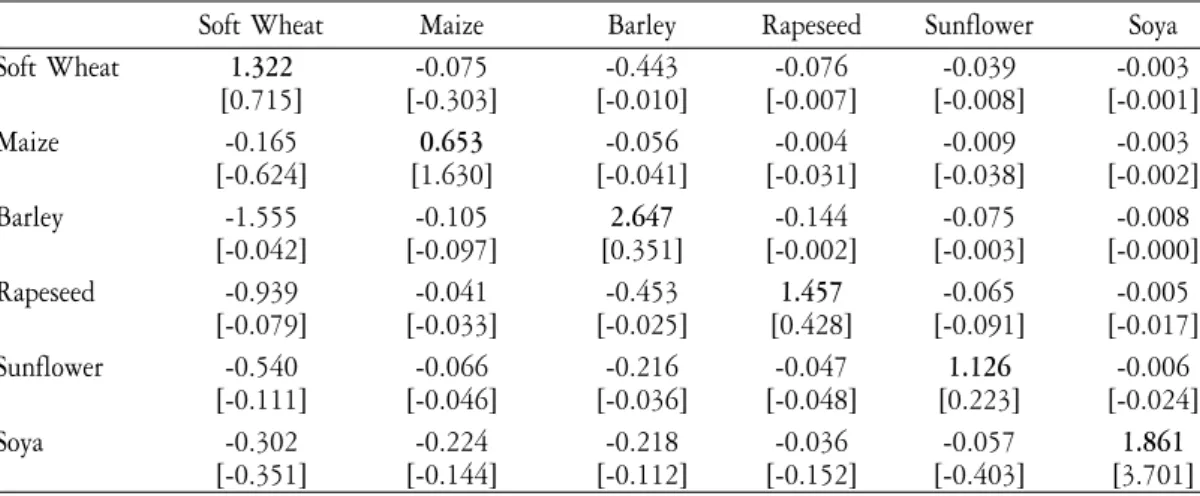
We started the evaluation of the results with simulation experiments based on partial 10 % increases of product prices and calculated the ag-gregated national percentage change in area related to the price change. Table 2 shows selected elasticities which are somewhat comparable to the « classical » econometric estimates provided by Guyomard et al. (1996) with respect to product differentiation and scope. The estimates of own priceelasticities are on average larger than their econometric counterparts (reported in brackets), but not uniformly so. The own price response of maize and soybeans is considerably below the values of Guyomard et al.. Generally, the estimated own price elasticities are smaller than the typical supply responses implied by LP’s or standard PMP-procedures (see for example Cypris, 2000 and the subsequent simulation exercise). Cross price

elasticities are also within the general magnitude of the econometric esti-mates, but they clearly show different structures of substitution between the crops. For example, with an increase of the soft wheat price, barley and rapeseed show the strongest (percentage) reductions in table 2. Those responses are rather small in the case of Guyomard et al., where maize is the main crop substituted by the increasing wheat production. One should not forget, however, that the theorical structure of the two under-lying models (fixed versus variable input and output coefficients) as well as the employed data base (cross sectional versus time series) differ bet-ween the two sets of estimates which limits their comparability.

Table 2. Price elasticities of supply for selected crops – National aggregate France

Soft Wheat Maize Barley Rapeseed Sunflower Soya

Soft Wheat 1.322 -0.075 -0.443 -0.076 -0.039 -0.003 [0.715] [-0.303] [-0.010] [-0.007] [-0.008] [-0.001] Maize -0.165 0.653 -0.056 -0.004 -0.009 -0.003 [-0.624] [1.630] [-0.041] [-0.031] [-0.038] [-0.002] Barley -1.555 -0.105 2.647 -0.144 -0.075 -0.008 [-0.042] [-0.097] [0.351] [-0.002] [-0.003] [-0.000] Rapeseed -0.939 -0.041 -0.453 1.457 -0.065 -0.005 [-0.079] [-0.033] [-0.025] [0.428] [-0.091] [-0.017] Sunflower -0.540 -0.066 -0.216 -0.047 1.126 -0.006 [-0.111] [-0.046] [-0.036] [-0.048] [0.223] [-0.024] Soya -0.302 -0.224 -0.218 -0.036 -0.057 1.861 [-0.351] [-0.144] [-0.112] [-0.152] [-0.403] [3.701]

Supply in rows and changed prices in columns. Reported elasticities are calculated as average percentage supply change (change in land allocation due to fixed yields) per one percent price change. The simulations are based on a 10 % increase in the respective crop prices. Values in brackets are the (rounded) supply elasticity estimates reported in Table 2 of Guyo-mard et al.(1996).

The comparison of the resulting partial supply responses with values of estimated behavioural functions is certainly interesting. However, the assessment of the simulation behaviour across larger economic and policy changes is closer to the ultimate purpose of our model. Therefore, we de-signed an ex-post simulation experiment as described above, results of which are rarely generated in the context of programming models, but are very informative from our point of view.

In order to judge if the new methodology has comparative advan-tages, we included a « standard PMP » approach in the ex-post valida-tion as well. Here, only diagonal elements of B are specified such that the linear and quadratic terms for each production activity i implicitly define average variable cost matching the observed accounting cost c_ifor the base year. In the case of the quadratic cost function this implies that

2λ_i

b_i,i = —— and d_i= c_i– λ_i ∀i = 1, ..., n (14)

x0_i

Furthermore, we defined an « intelligent no change » forecast by ta-king 1990 levels of annual crops reducing them – where applicable – by set-aside obligations. The resulting areas were then made consistent to the available land in 1994.

Figure 1 shows the percentage national deviation of « simulated » production activity levels from the observed activity levels in 1994 for the three approaches. The « standard approach » shows rather high de-viations for some major crops. Somewhat surprising, the « no-change » forecast is comparatively close to observed production activity levels. Apparently – the 1992 CAP-reform had – at least in France – a relati-vely small impact on the aggregate crop rotation apart from the set-aside Figure 1.

Percentage deviation of simulated from observed production activity levels for France

Sun flower seeds

effect. With this in mind, the fit of the ME-PMP approach based on the cross sectional sample is rather promising : apart from sunflowers and potatoes it provides better simulated values than the « no-change » re-sults. The sum of absolute deviation in levels weighted by the observed levels amounts just up to 3 % (see « Total »).

However, the variation in regional forecasting errors is at least of the same importance. The results in figure 1 could be a rather « lucky » out-weighing of regionally large under- and overestimating of activity levels. Therefore, we additionally checked the regional fit by calculating mean absolute percentage deviations over regions presented for the most im-portant activities and aggregates in figure 2. The standard approach was again no real competitor. However, the performance of the ME-PMP ap-proach is about the same as « no-change » apart from the aggregate of fallow land and set-aside. As explained above, problems could be expec-ted here as no substantial information entered the calibration step.

CONCLUSIONS

So far, most PMP application in aggregate programming models suf-fered from a rather arbitrary specification of the non-linear objective function. Classical econometric approaches cannot be applied to this ty-pically underdetermined estimation problem, a problem overcome by using the Maximum Entropy criterion as proposed in Paris and Howitt (1998). Their application, however, included just one observation on marginal cost and additionally suffered from a non-intuitive definition of supports based on their specific approach to ensure the correct curva-ture of the estimated cost function.

These problems were addressed by the ME-PMP approach presented in this paper which uses a cross-sectional sample in order to derive Figure 2.

Mean absolute percentage deviations of simulated from observed production activity levels across regions

Sun flower seeds

changes in marginal cost based on observed differences between regions with different crop rotations and provides a solution for the curvature problem with limited computational burden and direct definition of support points for the parameters of interest.

An ex-post validation of the resulting model specification simulated the 1992 CAP-reform for crop production in France. The results show a promising fit of observed production activity levels – not only for the national aggregate, but as well in the regional dimension. The ex-post simulation exercise – rarely executed or published in the context of ag-gregate programming models – shows the validity of the calibration procedure for regional programming models. The allocation behaviour of the resulting models is clearly superior to a standard application of PMP. Nevertheless, the general approach leaves ample opportunities for further research : Specific issues on our research agenda are the additio-nal use of time series observations to extend the information base and to estimate time dependant parameters, the introduction of estimated para-meters to describe the relationship between crop rotation and changes in marginal cost and, last but not least, an explicit elaboration on the links between PMP and duality based econometric models with explicit allo-cation of land to different production activities. The last issue could po-tentially improve the theoretical understanding of PMP which origina-ted as a rather pragmatic solution to calibration problems with agricultural programming models.

REFERENCES

ARFINI (F.), PARIS (Q.), 1995 — A positive mathematical

program-ming model for regional analysis of agricultural policies, in: SOTTE (E.) (ed.), The Regional Dimension in Agricultural Economics

and Policies, EAAE, Proceedings of the 40th Seminar, June 26-28, Ancona, pp. 17-35.

BARKAOUI(A.), BUTAULT(J.-P.), 1999 — Positive mathematical

pro-gramming and cereals and oilseeds supply within EU under Agenda 2000, Paper presented at the 9th European Congress of Agricultural Economists, Warsaw, August.

CYPRIS(Ch.), 2000 — Positiv Mathematische Programmierung (PMP) im Agrarsektormodell RAUMIS, Dissertation, University of Bonn.

GILL (P. E.), MURRAY (W.) and WRIGHT (M. H.), 1989 — Practical

Optimisation, London, Academic Press.

GOHIN(A.), CHANTREUIL(F.), 1999 — La programmation

mathéma-tique positive dans les modèles d’exploitation agricole. Principes et importance du calibrage, Cahiers d’économie et sociologie rurales,

52, pp. 59-78.

GOLAN(A.), JUDGE(G.) and MILLER (D.), 1996 — Maximum Entropy Econometrics, Chichester, Wiley.

GOLUB (G. H.), VAN LOAN(C. F.), 1996 — Matrix Computations, 3rd edition, Baltimore, John Hopkins University Press.

GRAINDORGE (C.), DE FRAHAN(B.-H.) and HOWITT (R. E.), 2001 — Analysing the effects of Agenda 2000 using a CES calibrated model of Belgian agriculture, in :HECKELEI(T.), WITZKE(H. P.) and HENRICHSMEYER(W.) (eds), 2000, Agricultural Sector Model-ling and Policy Information Systems, Proceedings of the 65th EAAE Seminar, March 29-31, 2000, Kiel, Wissenschaftsverlag Vauk, pp. 177-186.

GUYOMARD(H.), BAUDRY(M.) and CARPENTIER(A.), 1996 — Esti-mating crop supply response in the presence of farm programmes : application to the CAP, European Review of Agricultural Economics, 23, pp. 401-420.

HECKELEI(T.), 1997 — Positive mathematical programming : Review

of the standard approach, CAPRI-working paper 97-03, Univer-sity of Bonn.

HECKELEI(T.), BRITZ(W.), 2001 — Concept and explorative

applica-tion of an EU-wide regional agricultural sector model (CAPRI-Projekt), in: HECKELEI (T.), WITZKE (H. P.), and HENRICHS -MEYER (W.) (eds), Agricultural Sector Modelling and Policy

Information Systems, Proceedings of the 65th EAAE Seminar, March 29-31, 2000, Kiel, Wissenschaftsverlag Vauk, pp. 281-290. HELMING(J. F. M.), PEETERS (L.) and VEENDENDAAL(P. J. J.), 2001

— Assessing the consequences of environmental policy scenarios in Flemish agriculture, in: HECKELEI(T.), WITZKE (H. P.), and HENRICHSMEYER(W.) (eds), Agricultural Sector Modelling and Po-licy Information Systems, Proceedings of the 65th EAAE Seminar, March 29-31, 2000, Kiel, Wissenschaftsverlag Vauk, pp. 237-245.

HORNER(G. L.), CORMAN(J.), HOWITT(R. E.), CARTER(C. A.) and MACGREGOR(R. J.), 1992 — The Canadian regional agriculture model : Structure, operation and development, Agriculture Ca-nada, Technical Report 1/92, Ottawa.

HOUSE(R. M.), 1987 — USMP regional agricultural model,

Washing-ton DC, USDA, National Economics Division Report, ERS, 30. HOWITT(R. E.), 1995a — Positive mathematical programming,

Ame-rican Journal of Agricultural Economics, 77 (2), pp. 329-342. HOWITT (R. E.), 1995b — A calibration method for agricultural

eco-nomic production models, Journal of Agricultural Economics, 46, pp. 147-159.

HOWITT (R. E.), GARDNER (D. B.), 1986 — Cropping production and resource interrelationships among California crops in response to the 1985 food security act, in : Impacts of Farm Policy and Tech-nical Change on US and Californian Agriculture, Davis, pp. 271-290. KASNAKOGLU (H.), BAUER (S.), 1988 — Concept and application of an agricultural sector model for policy analysis in Turkey, in :

BAUER(S.), HENRICHSMEYER(W.) (eds), Agricultural Sector Mo-delling, Kiel, Wissenschaftsverlag Vauk.

LENCE(H. L.), MILLER(D.), 1998a — Estimation of multioutput

pro-duction functions with incomplete data : A generalized maximum entropy approach, European Review of Agricultural Economics, 25, pp. 188-209.

LENCE (H. L.), MILLER (D.), 1998b — Recovering output specific in-puts from aggregate input data : A generalized cross-entropy ap-proach, American Journal of Agricultural Economics, 80 (4), pp. 852-867.

LÉON(Y.), PEETERS (L.), QUINQU(M.) and SURRY(Y.), 1999 — The use of maximum entropy to estimate input-output coefficients from regional farm accounting data, Journal of Agricultural Econo-mics,50, pp. 425-439.

MITTELHAMMER(R. C.), CARDELL(S.), 2000 — The data-constrained GME-estimator of the GLM : Asymptotic theory and inference, Working paper of the Department of Statistics, Washington State University, Pullman.

MITTELHAMMER(R. C.), JUDGE(G. G.) and MILLER(D. J.), 2000 —

Econometric Foundations, New York, Cambridge University Press. OUDE LANSINK(A.), 1999 — Generalized maximum entropy and

he-terogeneous technologies, European Review of Agricultural Economics, 26, pp. 101-115.

PARIS(Q.), HOWITT(R. E.), 1998 — An analysis of ill-posed produc-tion problems using maximum entropy, American Journal of Agri-cultural Economics, 80-1, pp. 124-138.

PARIS (Q.), MONTRESOR (E.), ARFINI (F.) and MAZZOCCHI (M.),

2000 — An integrated multi-phase model for evaluating agricul-tural policies through positive information, in: HECKELEI (T.),

WITZKE (H. P.), and HENRICHSMEYER (W.) (eds), Agricultural

Sector Modelling and Policy Information Systems, Proceedings of the 65th EAAE Seminar, March 29-31, 2000, Kiel, Wissenschaftsver-lag Vauk, pp. 101-110.

PRECKEL (P. V.), 2001 — Least squares and entropy : A penalty func-tion perspective, American Journal of Agricultural Economics, 83-2, pp. 366-377.

SCHMITZ (H. J.), 1994 — Entwicklungsperspektiven der

Landwirt-schaft in den neuen Bundesländern Regionaldifferenzierte Simula-tionsanalysen, Alternativer Agrarpolitischer Szenarien, Studien zur Wirtschafts — und Agrarpolitik, Bonn, Witterschlick.

VAN AKKEREN (M.), JUDGE (G. G.) and MITTELHAMMER (R. C.), 2001 — Coordinate based empirical likelihood-like estimation in ill-conditioned inverse problems, Working paper of the University of California, Berkeley and Washington State University, Pullman. ZHANG (X.), FAN (S.), 2001 — Estimating crop-specific production

technologies in Chinese agriculture : A generalized maximum en-tropy approach, American Journal of Agricultural Economics, 83-2, pp. 378-388.