Binary Affinity Genetic Algorithm

(1)

Binary Affinity Genetic Algorithm

∗

Xinchao Zhao

School of Sciences, Beijing University of Posts and Telecommunications, Beijing, 100876, China [email protected] and [email protected]

Xiao-Shan Gao

KLMM, Institute of Systems Science, AMSS, Academia Sinica, Beijing, 100080, China

Abstract

Based on certain phenomena from the human society and nature, we propose a binary affinity genetic algorithm (aGA) by adopting the following strategies: the population is adaptively updated to avoid stagnation; the newly generated individuals are guaranteed to survive for certain number of generations in order for them to have enough time to develop their good genes; new individuals and the old ones are balanced to take both of their advantages. In order to quantitatively analyze the selective pressure, the concept ofselection degreeand a simple linear control equation are introduced. We can maintain the diversity of the evolutionary population by controlling the value of the selection degree. The performance of aGA is further enhanced by incorporating local search strategies. Keywords: genetic algorithm, selection degree, individual flowing, population diversity, global optimization.

1 Introduction

Genetic algorithms (GAs) refer to the meta-heuristical usage of the concepts, principles, and mechanisms about the natural evolution to solve problems [Holland (1975), Goldberg (1989), Michalewicz (1996)]. Most existing researches on GAs focused on the process of natural selections and genetics [Back and Fogel (1997)]. Computational methods based on socio-behavioral models [Jin and Reynolds (1999)] are recently introduced, which are inspired by the fact that individuals adapt and evolve faster through social ideas and deeds than through genetic inheritances. Along this line, Huang et al [Huang and Jin (1997)] proposed a quasi-physical personification algorithm to solve SAT problems by simulating personal behaviors. Reynolds and Chung [Reynolds and Chung (1997)] introduced an algorithm based on socio-behavioral dynamics. Ray and Liew [Ray and Liew (2003)] proposed an optimization algorithm by simulating social interactions.

The “premature convergence” is a major problem in GAs [Goldberg (1989), Zhou and Sun (1999)], which means that the population has already been homogeneous before finding the optimal solutions of the problem. The loss of critical alleles due to the selection pressure, the selection noise, the schemata disruption, and the poor setting of parameters may make the exploration balance disproportionate and hence lacking diversity in the population [Kuo and Huwang (1996), Mahfoud (1995), Potts and Giddens (1994)]. Many researches focused on the improvement of operators and parameter settings of GAs [Huang and Lim (2003), Schaffer and Caruana (1989)]. Another approach for dealing with this problem is the distributed GA model [Herrera and Lozano (2000)], which keeps, in parallel, several independent sub-populations processed by distinct GAs.

In this paper, we propose new ideas to deal with the premature convergence, which are inspired by a bio-scientific literature [Williams (1996)] and the following social phenomena:

1. Suppose that a colony consists of hawk individuals and pigeon individuals. A colony consisting of pigeons only is not steady because once a hawk is introduced, it will tyrannize its partners. On the other hand, a colony consisting of hawks only is not steady either, because all hawks commit aggressions against each other for foods ∗_{Partially supported by a National Key Basic Research Project of China and by a USA NSF grant CCR-0201253.}

(2)

and spouses. An “evolution steady strategy” [Williams (1996)] is to put pigeons and hawks according to aspecific proportionto the colony.

2. A Chinese proverb says: “running water does not get stale; a door-hinge is never worm-eaten.”

3. The new infants will be protected when they are added into a society full of hostility. Otherwise, they are certain to die. If they live in an inter-cooperative circumstance, they will do their best to prepare for their life in the future as quickly as possible.

4. If a rather good, but not the best “old man” (parental individual) and a new-graduated “young person” (newly produced individual) simultaneously appear at the personnel administration office, what should we do? One option is to ask them to do the same work at a cooperative as well as competitive niche. The old man with beneficial experiences and the young man full of youthful spirits will promote and support each other. After a certain period of time, we choose the best one as the “offspring”.

Inspired by the first and second phenomena, the population in the GA is adaptively updated from time to time when it “crowds”. This will make the searching engine energetic. Otherwise, stagnation may occur. Inspired by the third phenomenon, the newly generated individuals will be ensured to survive for a certain number of generations. In this way, they have enough time to show their good genes and build potential good gene blocks [Holland (1975)]. Inspired by the fourth phenomenon, we will keep a balance between the new individuals and the old ones when updating the population. Since the above strategies are full of humanitarianism, our proposed algorithm is named as the affinity genetic algorithm (aGA).

In order to quantitatively analyze the selective pressure, the concept ofselection degreeand a simple linear control equation are introduced. We can maintain the evolutionary population diversity by controlling the value of the selection degree.

An improved affinity genetic algorithm (iaGA) is further proposed by incorporating local search methods from [Huang and Lim (2003)] into the aGA.

Seventeen global optimization benchmark functions are used to compare the simple genetic algorithm (SGA), aGA, and iaGA. Experiments show that the performance of aGA is much better than that of SGA [Goldberg (1989)], and the performance of iaGA is much better than that of aGA.

The rest of this paper is organized as follows. Section 2 introduces the affinity genetic algorithm. Section 3 describes the benchmark optimization problems. Section 4 makes comparisons among SGA, aGA, and iaGA by solving the benchmarks. Finally, conclusions are made in Section 5.

2 Affinity Genetic Algorithm

2.1 Overview of Genetic Algorithm

The GA is a metaphoric abstraction of natural biological evolution. The basic concepts providing the underlying foun-dation for GAs are natural selection, recombination (crossover), and mutation [Goldberg (1989), Michalewicz (1996), Zhou and Sun (1999)]. Natural selection is the process by which chromosomes containing better encodings have a greater probability of reproducing than those who have weaker encodings. The SGAs [Goldberg (1989), Zhou and Sun (1999)] are guided largely by three operators: reproduction, crossover, and mutation [Michalewicz (1996), Zhou and Sun (1999)]. The chromosome in the SGA is typically encoded as a binary string with an allele value of 0 or 1 at each bit position. Recently, a multiple bit encoding-based search algorithm [Zhao and Long (2005)] is proposed which outperforms the single representation-based search algorithm. To find a solution to a problem, the SGA randomly creates an initial population with each chromosome in it representing a possible solution. Through the natural selection, chromosomes encoded with better possible solutions are chosen for recombination, yielding improved offsprings for successive genera-tions. Natural evolution of the population continues until a predetermined number of generations is reached, resulting in a final generation of highly fit chromosomes representing the optimal or near optimal solutions to the problem.

(3)

2.2 Population Diversity and Selective Pressure of SGA

It is well known that theselective pressure andpopulation diversity are two important issues in the evolution process of GAs. These two factors are strongly related: an increase in the selective pressure reduces the population diversity and vice versa [Michalewicz (1996)]. In other words, strong selective pressure “supports” the premature convergence of the GA search; a weak selective pressure can make the search ineffective. The sampling mechanism

[De Jong (1975)], the elitist model, and the expected value model [Whitley (1989)] are proposed to keep the balance between these two factors.

Kim et al [Kim (2003)] indicated that the population diversity is of utmost importance to promote a more thorough test of individuals and a more reliable evaluation of fitness. They introduced the concept of Population Diversity (D)to measure the diversity for a binary encoded GA as follows:

D= 2nP−1 i=1 n P j=i+1 Hi,j n(n−1)l ,

wherenis the population size,lis the length of the binary individual, andHi,j is the hamming distance between two individualsi andj.

The convergence of GAs is one of the most challenging theoretical issues in the evolutionary computation area. Gold-berg and Segrest [GoldGold-berg (1989)] provided a finite Markov chain analysis of GAs (for finite population, reproduction, and mutation only GAs). Based on the Banach fix point theorem, Szalas and Michalewicz [Szalas and Michalewicz (1993)] explained the convergence properties of GAs. To measure the convergence rate, we define the concept ofSelection

Degree (SD) as follows

SD= Number of Super Individuals Population Size

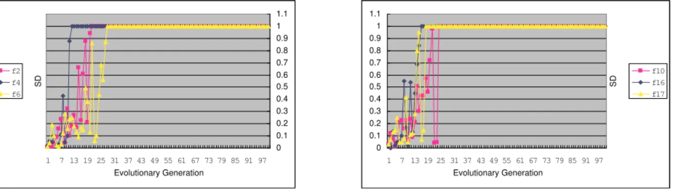
where a “super individual” is one of the best individuals in the population, both before and after the selection. From the above discussion and the definitions ofDandSD, we conclude thatDis strongly influenced bySDand SDis closely related to the convergent rate of GAs. However, the SGA usually becomes homogeneous before the global optimal solution is found. In other words, the SDof SGA is so high that its population diversityD is very low and evolutionary stagnation occurs when it only explores a small portion of the search space. This phenomenon is shown in Figure 1 with some experiments. Functionsf2, f4, f6, f10are 2 and 4 dimensional multimodal functions respectively

with only a few local minima andf16, f17are multlmodal functions with many local minima. The population size and

the maximal evolutionary generation are both 100 in this group of experiments and other parameters are the same as those in Section 3. Note that the number of super individuals are counted afterthe selection operation.

1 7 13 19 25 31 37 43 49 55 61 67 73 79 85 91 97 Evolutionary Generation S D 0 0.1 0.2 0.3 0.4 0.5 0.6 0.7 0.8 0.9 1 1.1 f2 f4 f6 0 0.1 0.2 0.3 0.4 0.5 0.6 0.7 0.8 0.9 1 1.1 1 7 13 19 25 31 37 43 49 55 61 67 73 79 85 91 97 Evolutionary Generation S D f10 f16 f17

Figure 1: SDvs evolutionary generations for SGA. (L) functionf2, f4, f6 (R) functionsf10, f16, f17

From Figure 1, we can see thatSDapproaches to one quickly (population is full of super individuals) for all functions. This meas that the crossover operator has lost its effectiveness after about 30 generations. But it is well known that the crossover operator is the main operator for GAs [Holland (1975), Michalewicz (1996), Zhou and Sun (1999)]. This fast evolutionary stagnation phenomenon of SGA leads us to study how to control the selective pressure and the genetic diversity. In this paper, we will give a simple linear mathematical model for the selective pressure which will be discussed in the next subsection.

(4)

2.3 A Linear Model for the Selective Pressure

Figure 1 shows that the selective degree SDof the SGA is so high that it has already lost its genetic diversity after it evolves a small number of generations. Inspired by certain natural and social phenomena, we propose a simple model to control the number of super individuals to overcome the population homogenous problem. The mathematical model for the selective pressure in the GA is given below. Refer to the next subsection for all the parameters used in Eq.(1).

SD= SD0+ 1 +generation−G0

1 +GENERATION−G0×incrSD0 (1)

The model is used to control the excessive reproduction of super individuals once the parameter SD exceeds a predetermined proportion (SD0). After that, SD only increases ( incrSD0

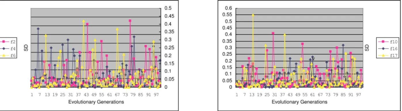
1+GENERATION−G0) with the augment of each evolutionary generation. With the evolution of GA, the allowed proportion of super individuals is larger and larger. Finally, it reaches the allowedmaximal proportion in the population, i.e.,SD=SD0 +incrSD0. In order to show the effects of the selective pressure, Figure 2 illustrates the relationship betweenSDand the evolutionary generations.

1 7 13 19 25 31 37 43 49 55 61 67 73 79 85 91 97 Evolutionary Generations S D 0 0.05 0.1 0.15 0.2 0.25 0.3 0.35 0.4 0.45 0.5 f2 f4 f6 0 0.05 0.1 0.15 0.2 0.25 0.3 0.35 0.4 0.45 0.5 0.55 0.6 1 7 13 19 25 31 37 43 49 55 61 67 73 79 85 91 97 Evolutionary Generations S D f10 f16 f17 v

Figure 2: SDvs evolutionary generations for aGA (L) functionf2, f4, f6(R) functionsf10, f16, f17

From Figure 2, we find that the population of the aGA has a very good genetic diversity, i.e, a varying selective pressure. Comparing Figures 1 and 2, we could see the effects of our proposed strategies. Of course, the model proposed by us is very simple. More work should be done on this problem so that we could have a deeper understanding for the evolution behavior of GAs.

2.4 The Affinity Genetic Algorithm

The affinity genetic algorithm (aGA) is based on the framework of SGA [Goldberg (1989)]. Similar to SGA, the aGA adopts the binary encoding, two points crossovers, uniform mutations, tournament selections (for minimizing and tournament size = 2), and the elitism. The traditional tournament selection is to choose the better one as the offspring from two chosen individuals. If the two chosen individuals have equal fitness, one is randomly chosen from them. The tournament selection will be modified below.

In the following algorithm, the word “age” means the number of generations that one individual has survived in the population. The “infants” refer to the newly-generated individuals or those whose age is less than or equal to a predetermined constantAGE. Once the “age” of an individual is larger thanAGE, it becomes a grown up. A “niche” is initially formed by two individuals (one infant and one grown up). A crossover operation is applied to them and two new individuals are obtained. Two of the best individuals are selected from those four individuals as the offsprings in this niche subsequently. This process iterates for a predefined number of times and a best individual obtained from this niche is added into the current population.

Now, we give the modified tournament selection procedure.

1. Two individuals are randomly chosen for the tournament selection. We suppose that not both of them are “too poor”.

(5)

(a) Two chosen individuals are both infants or both grown ups: the algorithm chooses the better one as the offspring if their fitness are not equal. If the two individuals are the same, then the current population “crowds” to some extent. A new individual is introduced and its “age” is initialized as zero. Otherwise, we have two different individuals with the same fitness. In this case, one of two is randomly chosen to the next generation.

(b) One individual is an infant and the other is a grown-up: the algorithm directly chooses the infant as the offspring if the fitness of the grown up is below the average level of the current population. Otherwise, the infant and the grown-up form a niche and then exchange their inherent materials (genes) for some generations. There are many individuals in this niche, including the newly-produced children and two parents. Then a best one is chosen as the offspring.

3. Scan the current population after the selection and count the the number of occurrences of the best individuals for current population. If a best individual is not chosen, elitist model is applied. If the adaptively updated proportion of the best individuals is exceeded, that is, the super individuals are too crowded, then some super ones will be replaced by equal number of newly-produced individuals (“infants”). The “infants” are protected and their “ages” are initialized as zero.

Another modification is the crossover condition. Crossovers occur in standard GAs if a random decimal fraction is less than the crossover probability. Besides the above condition, crossovers occur if at least one of the individuals in the crossover pair is an infant. The reason to do this is to make the infants exchanging inherent information with grown ups as quickly as possible, which corresponds to the third inspiring idea of Section 1. This also makes the infants mature and the genes of other individuals in the population to be updated from time to time. Finally, if the ages of the infants are larger than the predetermined constant AGE, they become grown ups and unprotected. Otherwise, their ages are added by one.

We define “better”, “equal”, and “worse” individuals as follows. Suppose that a precision of six digits after the decimal point meets the demand of computation. Then, a variable x=ZERO means that x∈[−10−6_,₁₀−6_{]. An}

individual 1 is “better” (“worse”) than an individual 2 if f itness1−f itness2≤ −ZERO(or f itness1−f itness2≥

ZERO) (for minimization). The fitness values of two individuals are “equal” ifabs(f itness1−f itness2)< ZERO.

Two individuals are treated as the “same” if their corresponding real components are almost the same. Two real numbers r1 andr2 are almost the same if the absolute value of (r1−r2) is less thanZERO.

The global constants used in the GAs are given below. POPSIZEis the population size;GENERATIONis the maximal evolution generation; generation is the evolution loop variable; PC, PM are the crossover and mutation probabilities respectively; SDis the adaptively updating selective degree;SD0 is the predetermined initial selective pressure;G0is the evolution generation number from which the excessive reproduction of super individuals begins to be controlled; incrSD0 is the permitted maximal super individuals increment. The pseudo-code of the tournament selection of the aGA is presented below.

Procedure of Tournament Selection

AVERAGE, WORST: the average and worst fitness in the current population

1. Find the best and worst individuals and compute the average fitness (AVERAGE) before selection 2. Randomly select two individuals from the population

3.1 Randomly produce a decimal fractionrbetween 0 and 0.5

3.2DISTANCE=AVERAGE- (1 - r)×(AVERAGE-WORST)

3.3 While (both fitness of two individuals<DISTANCE) randomly select another individual

4. if (both individuals are infants or grown ups)

4.1 if their fitness are not equal then choose the better one as the offspring

4.2 if they are the same individual then generate a new one as offspring and protect it

4.3 if they are distinct individuals with the same fitness then randomly select one from them as the offspring 5. if (one being an infant and the other a grown up)

5.1 if (the fitness of the grown-up<AVERAGE) then choose the infant as the offspring

5.2 else form a niche with them and exchange inherent information for two times. Finally, the best individual is chosen in this niche as the offspring

(6)

7. Find the worst individuals (WORST) from current population and count the number of the best individual

(NUMBER) to computeSD

8. if the best individual is not being selected then execute elitism 9. if (selective degreeSDexceedsSD0 for the first time) then

G0= the current generation 10. if (G0>0) then

10.1SD= SD0+₁₊1+_GENERATIONgeneration−G0₋_G0×incrSD0

10.2HAWK1_{= (}_int₎₍_POPSIZE_×_SD₎

10.3 ifNUMBER>HAWKthen randomly replace (NUMBER -HAWK) super individuals by equal number of new individuals and protect them

End Tournament Selection

The pseudo-code of the affinity genetic algorithm is presented as follows.

Procedure of aGA(for minimization)

1. Initialize all necessary parameters

2. Randomly produce the initial population, P(0) 3. Evaluate P(0);

4. Initialize variable generation = 1

5. Tournament selection

6. Two-point crossover

if (rand2_<_PC_{) or (}_{either of the crossing pair is an infant}₎

6.1 implement two-point crossover;

6.2 if the age of infants are larger than the predefinedAGEthen they become grown-ups; 6.3 else the age of infants add by one;

7. Mutate

8. Evaluate current population

9. Generation←generation+ 1;

10. ifgeneration≤GENERATIONthen goto 5 else output solution and quit; End Procedure of aGA

2.5 Improved Affinity Genetic Algorithm (iaGA)

The mathematical model of Eq.(1) effectively controls the genetic diversity and avoids the prematurity of GAs. Due to the interactive relationship between the genetic diversity and the selection pressure [Michalewicz (1996)], the selection pressure of the aGA population will be reduced. In order to make the algorithms more effectively convergent, local searches are incorporated into GAs. Huang and Lim [Huang and Lim (2003)] proposed a hybrid GA to solve the linear ordering problem and obtained quite good results. Davis [Davis (1991)] proposed a Random Bit Climber (RBC) algorithm which is a next descent hill-climbing algorithm. The search starts from a random bit string, and proceeds by testing each of the Hamming-1 neighbors in some randomized order. Both equal and improved moves are accepted. If the search is stuck in a local optimum, the algorithm re-starts from a new random bit string.

However, local searches are used to every individual in the process, which is costly. In order to improve the performance of aGA, we use the local searches for every ten generations to improve the best individuals and the medial individuals which are better than and most close to the average fitness of the current population. The reason that we improve individuals in every ten generations is that the best and the median individuals should have been changed after involution of ten generations. Otherwise, they may not have enough change. The idea of improving the medial individual comes from the fact that the best individual has a high probability to be trapped by a “basin of attraction”(including the global optimal basin). Hence, local searches have no effects in this situation and the medial individuals do not have this problem. Furthermore, the parents and offsprings in the crossover and mutation operations compete with each other [Zhao (2005)] and the better ones are put into the next generation.

As far as the local search is concerned, it is applied to the decoded phenotypic variables (real-coded vectors), which has no effects on the genotype bit-strings. The decoded real-coded vector Xis obtained from the best or the

1_{An integer is less than, but is closest to the factual value of super individuals over}_POPSIZE_. 2_{a uniform random float number between 0 and 1}

(7)

median binary individuals. The pseudo-code of the local search on the real-coded vector is as follows, wheremis the dimensions of the real vectors,LOOPis the executing times of the local search,Nj1(0,1) andNj2(0,1) are the normally

distributed one-dimensional random numbers with mean zero and standard deviation one. They are generated anew for each value ofj.

Procedure of Local Search

Find the best (u) and median (v) individuals of the current population; Decode the binary stringsu,vinto real vectorsruandrv;

for (i = 1; i<=LOOP; i++) for (j=1; j<=m; j++)

ru0[j] =ru[j] +Nj1(0,1);

rv0[j] =rv[j] +Nj2(0,1);

if fitness ofru0 is not worse than that ofruthen ru=ru0;

if fitness ofrv0 is not worse than that ofrvthen rv=rv0;

End Procedure

where rv[j] is thejth-component ofrv.

3 Benchmark Functions

Benchmark functions chosen from [Yao and Liu (1999), Zhou and Sun (1999)] are all minimization problems. A large number of benchmarks is necessary because Wolpert and Macready [Wolpert and Macready (1997)] have shown that under certain assumptions no single search algorithm is best on average for all problems. If the number of benchmarks is too small, it would be very difficult to make a generalized conclusion and have the potential risk that the algorithm is biased toward the chosen problems. Functionsf1, . . . , f12are low-dimensional functions which have only a few local

minima andf13(n = 5) is a high-dimensional and unimodal function [Yao and Liu (1999)]. Functionsf14, . . . , f17(n =

5) are mutilmodal functions where the number of local minima increases exponentially with the augment of the problem dimensions. They are the most difficult class of problems for many optimization algorithms [Yao and Liu (1999)]. The fact that all the benchmarks except f13 are multlmodal functions is very important because the final results

of these functions reflect an algorithm’s ability of escaping from poor local optima and locating a global optimum [Yao and Liu (1999)]. The benchmark functions are given below.

Bohachevsky Function #1

f1=x21+ 2x22−0.3cos(3πx1)−0.4cos(4πx2) + 0.7, -50≤xi≤50. min(f1) = f1(0, 0) = 0.

Bohachevsky Function #2

f2=x21+ 2x22−0.3cos(3πx1)cos(4πx2) + 0.3, -50≤xi≤50. min(f2) =f2(0, 0) = 0.

Bohachevsky Function #3 f3=x21+ 2x22−0.3 cos(3πx1+ 4πx2) + 0.3, -50≤xi ≤50. min(f3) =f3(0, 0) = 0. Shubert function f4= 5 P i=1 icos[(i+ 1)x1+i]× 5 P i=1 icos[(i+ 1)x2+i], -10≤xi≤10. min(f4) = -186.73. Schaffer Function f5= 0.5 + sin2√_x2 1+x22−0.5 (1.0+0.001(x2 1+x22))2, -100≤xi≤100. min(f5) =f5(0, 0) = 0. N. Kowalik’s Function f6= 11 P i=1 [ai−x1(b2i+bix2) b2 i+bix3+x4] 2_{, -5}_≤_xi_≤_{5, min(}_f

6)= 0.0003075 at (0.1928, 0.1908, 0.1231, 0.1358). The coefficients can

be followed in Table 1. Colville Function

(8)

i 1 2 3 4 5 6 7 8 9 10 11 ai 0.1957 0.1947 0.1735 0.1600 0.0844 0.0627 0.0456 0.0342 0.0323 0.0235 0.0246 b−1

i 0.25 0.5 1 2 4 6 8 10 12 14 16

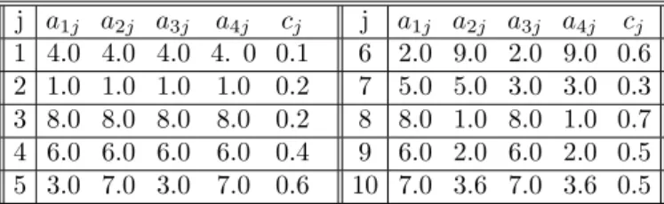
Table 1: Coefficients of N. Kowalik’s Function j a1j a2j a3j a4j cj j a1j a2j a3j a4j cj 1 4.0 4.0 4.0 4. 0 0.1 6 2.0 9.0 2.0 9.0 0.6 2 1.0 1.0 1.0 1.0 0.2 7 5.0 5.0 3.0 3.0 0.3 3 8.0 8.0 8.0 8.0 0.2 8 8.0 1.0 8.0 1.0 0.7 4 6.0 6.0 6.0 6.0 0.4 9 6.0 2.0 6.0 2.0 0.5 5 3.0 7.0 3.0 7.0 0.6 10 7.0 3.6 7.0 3.6 0.5

Table 2: Coefficients of Shekel SQRN5, SQRN7 and SQRN10 Functions

f7 = 100(x2−x21)2+ (1−x1)2+ 90(x4−x23)2+ (1−x3)2+ 10.1((x2−1)2+ (x4−1)2) + 19.8(x2−1)(x4−1),

-10≤xi≤10, min(f7)= 0 at (1, 1, 1, 1).

Shekel SQRN5, SQRN7 and SQRN10 function f8=s3(x1, x2, x3, x4) =− 5 P j=1 1 4 P i=1 (xi−aij)2₊_cj ,f9=s4(x1, x2, x3, x4) =− 7 P j=1 1 4 P i=1 (xi−aij)2₊_cj f10=s5(x1, x2, x3, x4) =− 10 P j=1 1 4 P i=1 (xi−aij)2₊_cj , 0≤xi≤10.

The global minima of f8, f9 andf10 are -10.15320, -10.402820 and -10.53628 respectively at the point (4, 4, 4, 4).

The coefficients are given in Table 2. R. Hartman’s Family f11&f12=− 4 P i=1 ciexp[− n P j=1

aij(xj−pij)2] with n = 3, 6 respectively, where 0≤xi≤1, min(f11)= -3.86 at (0.114,

0.556, 0.852) and min(f12)= -3.32 at (0.201, 0.150, 0.477, 0.275, 0.311, 0.657). Coefficients are given in Table 3 &

Table 4. Schwefel’s Problem 2.22 f13 = n P i=1 |xi|+ Qn i=1

|xi|, -10≤xi ≤10. n = 5 and min(f13) =f13(0, . . . ,0) = 0.

Generalized Schwefel’s Problem 2.26 f14=−

n P i=1

(xisin(p|xi|)), -500≤xi≤500, n = 5 and min(f14)= -2094.9166 at (420.9687,. . .,420.9687).

Generalized Rastrigin’s Function f15=

n P i=1

[x2

i −10 cos(2πxi) + 10], -5.12≤xi≤5.12, n = 5 and min(f15)= 0 at (0,. . ., 0).

i aij, j= 1,2,3 ci pij, j= 1,2,3 1 3 10 30 1 0.3689 0.1170 0.2673 2 0.1 10 35 1.2 0.4699 0.4387 0.7470 3 3 10 30 3 0.1091 0.8732 0.5547 4 0.1 10 35 3.2 0.038150 0.5743 0.8828 Table 3: Coefficients of R. Hartman’s Function (n= 3)

(9)

i aij, j= 1, . . . ,6 ci pij, j= 1, . . . ,6

1 10 3 17 3.5 1.7 8 1 0.1312 0.1696 0.5569 0.0124 0.8283 0.5886 2 0.05 10 17 0.1 8 14 1.2 0.2329 0.4135 0.8307 0.3736 0.1004 0.9991 3 3 3.5 1.7 10 17 8 3 0.2348 0.1415 3522 0.2883 0.3047 0.6650 4 17 8 0.05 10 0.1 14 3.2 0.4047 0.8828 0.8732 0.5743 0.1091 0.381

Table 4: Coefficients of R. Hartman’s Function (n= 6)

Ackley’s Function f16=−20 exp(−0.2 s 1 n n P i=1 x2 i)−exp(1n n P i=1

cos(2πxi))+20+e, -32≤xi≤32, n = 5 and min(f16)= 0 at (0,. . .,0).

Generalized Griewank Function f17= ₄₀₀₀1 n P i=1 x2 i − n Q i=1 cos(√xi i)+1, -600≤xi≤600, n = 5 and min(f17)= 0 at (0,. . .,0).

4 Experimental Studies

The tournament selection, the two-point crossover, the uniform mutation, and the elitism [Back and Fogel (1997), Goldberg (1989), Zhou and Sun (1999)] are applied to SGA in this paper. Some comparisons for SGA, aGA, and iaGA based on the binary encoding GA are given. Algorithms are implemented by C programming language. The stopping criteria is to set the maximal evolution generations. All results are the statistical data which are based on 50 independent trials. It is widely known that the result of an incomplete algorithm may be improved by fine tuning parameters. In order to avoid such a bias, we will run the algorithms with a set of predefined parameters. We choose the following parameters for the algorithms without special statements. We use six digits after the decimal point as the computational precision. The experimental data are all collected according to this criterion. Let PC= 0.8, PM

= 0.05, AGE = 2, SD0 = 0.1,incrSD0 = 0.4,LOOP = 100. The population size of SGA istwiceof that of aGA and iaGA so that SGA has more exploring chances. The maximal evolutionary generations of the algorithms are the same. In aGA and iaGA, POPSIZE = 50 and GENERATION = 100 for functionsf1, . . . , f5 andf11, and POPSIZE

= 100 and GENERATION = 200 for other functions.

4.1 Performance Comparisons for SGA, aGA, and iaGA

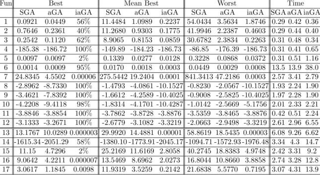
The experimental results are given in Table 5.

For the aGA, the results in the Mean BestandWorstcolumns illustrate its robustness and theBestcolumn shows the strong exploitation ability of the aGA which simulates the affinity ideas and social behaviors. Generally speaking, our affinity ideas and social behaviors simulation can significantly improve the exploration/exploitation capability of the SGA.

For the performance of the iaGA, we can see encouraging results for all benchmarks. First, the iaGA finds the global minima for 13 in 17 benchmarks. The results for functions f7, f13 andf16 are also very close to the global minima.

The iaGA greatly outperforms aGA and SGA in all benchmarks. Second, for five functionsf4, f8, f9, f11 andf12, the

iaGA finds their global minima in every run of the 50 trials, which shows the strong robustness of the iaGA. Third, the average running efficiency of iaGA ranges from one to four times of that of aGA and SGA. In a summary, the iaGA significantly increases the performance of aGA and SGA.

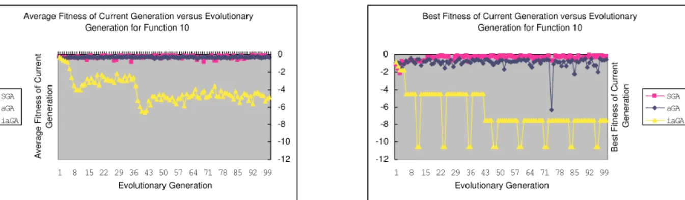
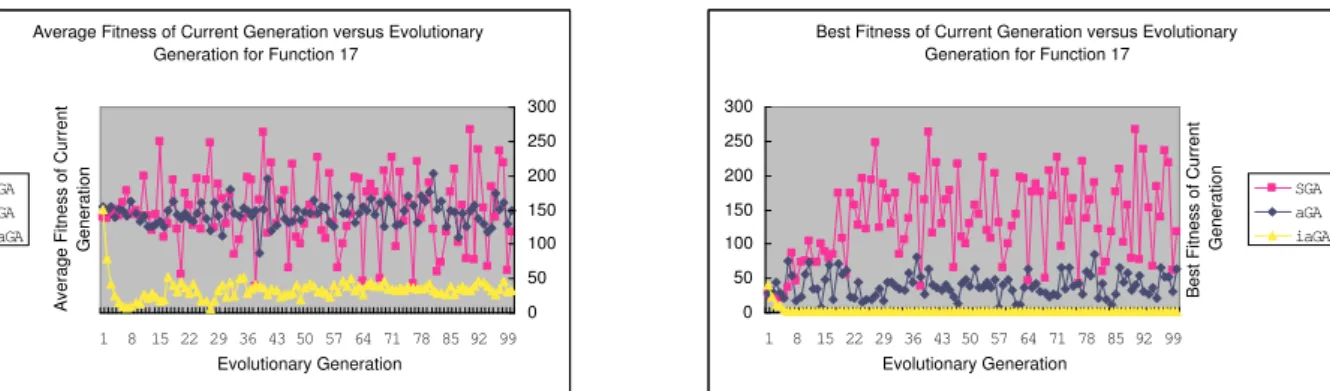
In order to compare SGA, iGA, and iaGA, four representative functions (out of 17) from each group are tested to show the relationship between the average and the best fitness versus the evolutionary generation. Functions f2, f10

are multimodal functions with only a few local minima and functions f16, f17 are multimodal functions with many

local minima.

From Figures 3-6 and Table 5, we find that iaGA outperforms the other two algorithms not only for the final statistical results, but also for the dynamic averages and the best fitness with the evolution of the genetic population.

(10)

Fun Best Mean Best Worst Time

SGA aGA iaGA SGA aGA iaGA SGA aGA iaGA SGA aGA iaGA

1 0.0921 0.0449 56% 11.4484 1.0989 0.2237 54.0434 3.5634 1.8746 0.29 0.42 0.36 2 0.7646 0.2361 40% 11.2680 0.9303 0.1775 41.9946 2.2387 0.4603 0.29 0.44 0.40 3 0.2542 0.1120 62% 8.9065 0.8153 0.0859 30.6782 2.3834 0.2263 0.31 0.48 0.34 4 -185.38 -186.72 100% -149.89 -184.23 -186.73 -86.85 -176.39 -186.73 0.31 0.41 0.65 5 0.0097 0.0097 2% 0.1339 0.0277 0.0128 0.3228 0.0868 0.0372 0.31 0.51 1.16 6 0.0014 0.0009 95% 0.0170 0.0018 0.0003 0.0449 0.0029 0.0008 13.5 13.9 38.0 7 24.8345 4.5502 0.00006 275.5442 19.2404 0.0001 841.3413 47.2186 0.0003 2.57 3.41 2.79 8 -2.8962 -8.7330 100% -1.4793 -4.0861 -10.1527 -0.8230 -2.0567 -10.1527 1.93 2.24 1.90 9 -3.4621 -7.8392 100% -1.6612 -4.2589 -10.4025 -0.9008 -2.5825 -10.4025 1.97 2.28 1.90 10 -4.2208 -9.4118 98% -1.8314 -4.1701 -10.4287 -1.0142 -2.5669 -5.1756 2.01 2.33 2.21 11 -3.8846 -3.8854 100% -3.7862 -3.8728 -3.8876 -3.5359 -3.8465 -3.8876 0.42 0.51 2.24 12 -3.1333 -3.2671 100% -2.6779 -3.1082 -3.3219 -2.0663 -2.9498 -3.3219 2.61 2.96 6.55 13 13.1767 10.0289 0.000003 29.9920 14.4881 0.00001 58.8619 18.5435 0.00003 6.08 9.26 6.62 14 -1615.34 -2051.29 58% -1380.10 -1773.91 -2045.17 -1094.71 -1572.93 -1976.48 3.34 4.3 14.7 15 11.15 4.7296 2% 25.2169 11.6169 2.8058 40.2745 18.8383 4.9748 2.42 3.31 9.2 16 9.0642 4.2211 0.000007 13.5469 8.6962 2.0273 16.8044 10.8660 3.8858 2.74 3.28 12.8 17 3.0617 1.1845 0.0098 11.9319 3.5259 0.2142 21.6838 5.5770 0.7195 3.07 4.31 13.9

Table 5: Performance comparisons among elitist SGA, aGA, and iaGA. TheBest(Worst) column is the best (worst) result in 50 runs. The Mean BestandTime are the average results in 50 trials. If the global optimum has reached, theBest column will represent the percentage of runs in which this happens.

For the aGA and SGA, we should comprehensively analyze the left and right figures for each function as well as Figure 2. Although in every generation the average fitness of aGA shows no superiority to SGA, the best fitness of aGA in each generation greatly outperforms SGA which exactly validates the effects of our new ideas. The super individuals are not allowed to abundantly propagate in the aGA, but not so in SGA. Therefore, once a super individual is introduced into the population of SGA, it will abundantly reproduce itself and at this time the average fitness of SGA is better than that of aGA. Otherwise, SGA is outperformed by aGA, for the population of aGA is an adaptively updated (individual flowing) and an evolutionary steady one which can also balance the “old” individuals and the newly introduced ones.

This series of experiments strongly validate the effectiveness of our idea that an evolutionary algorithm with adap-tively updating population and personnel administration experiences has much higher diversity as well as better experimental results than that of SGA.

Average Fitness of Current Generation versus Evolutionary Generation for Function 2

1 8 15 22 29 36 43 50 57 64 71 78 85 92 99 Evolutionary Generation A v e ra g e F it n e s s o f C u rr e n t G e n e ra ti o n 0 1000 2000 3000 4000 5000 6000 7000 SGA aGA iaGA

Best Fitness of Current Generation versus Evolutionary Generation for Function 2

0 1000 2000 3000 4000 5000 6000 7000 1 8 15 22 29 36 43 50 57 64 71 78 85 92 99 Evolutionary Generation B e s t F it n e s s o f C u rr e n t G e n e ra ti o n SGA aGA iaGA

Figure 3: Fitness of current generation of functionf2 vs evolutionary generation (L) Average (R) Best

4.2 Analyzing SD0 and incrSD0 of Linear Control Model

It is necessary to analyze how the initial parametersSD0and the augment of the super individualsincrSD0influence the convergence of GAs since thepopulation diversityandselective pressureare two main issues and the former

(11)

1 8 15 22 29 36 43 50 57 64 71 78 85 92 99 Evolutionary Generation A v e ra g e F it n e s s o f C u rr e n t G e n e ra ti o n -12 -10 -8 -6 -4 -2 0 SGA aGA iaGA

-12 -10 -8 -6 -4 -2 0 1 8 15 22 29 36 43 50 57 64 71 78 85 92 99 Evolutionary Generation B e s t F it n e s s o f C u rr e n t G e n e ra ti o n SGA aGA iaGA

Average Fitness of Current Generation versus Evolutionary Generation for Function f16

1 8 15 22 29 36 43 50 5764 71 78 85 92 99 Evolutionary Generation A v e ra g e F it n e s s o f C u rr e n t G e n e ra ti o n 0 5 10 15 20 25 SGA aGA iaGA

Best Fitness of Current Generation versus Evolutionary Generation for Function f16

0 5 10 15 20 25 1 8 15 22 29 36 43 50 5764 71 78 85 92 99 Evolutionary Generation B e s t F it n e s s o f C u rr e n t G e n e ra ti o n SGA aGA iaGA

is strongly influenced by the latter. Two typical functions,f2, f17, are chosen, one of which is multimodal with a few

local minima and the other with many local minima. All data are statistical results in 50 independent trials. SD0 ranges from 0.1 to 0.6 with a step of 0.1 andincrSD0 ranges from 0.4 to 1-SD0 in every case ofSD0. WhenSD0 is 0.1,incrSD0 has 6 cases (0.9, 0.8, ..., 0.4). In general, there are 21 (6+ 5+ ... + 1) cases in all the combinations

ofSD0andincrSD0. In Figure 7, the horizontal line represents the dualistic data array ofSD0andincrSD0. The

first (left most) group of results is for (SD0,incrSD0) = (0.1, 0.4), (0.1, 0.5), (0.1, 0.6), and so on. The last (right most) group is for (SD0,incrSD0) = (0.6, 0.4).

Figure 7 shows that the parameters of (SD0, incrSD0) = (0.1, 0.4) we adopted is not the best case for functions f2, f17 for the best, average, and worst results in the 50 trials. Although no statistically significant differences can

be found among all the cases, the 10th case (0.2, 0.7), however, performs a little better than other cases for the two functions.

5 Conclusions and Future Work

A new aGA is proposed based on ideas inspired by a bio-scientific literature, one natural phenomenon, and personnel administration experiences. Experiments conclude that the new ideas can effectively control the selective pressure and make population diverse. In order to quantitatively analyze the selective pressure, a new concept, selection

degree (SD), is also introduced, which is closely correlative to the evolutionary behavior of GAs. The population

diversity can be effectively controlled through a linear control equation given in this paper. Generally speaking, an adaptive updating evolutionary algorithm with the “experience of personnel administration” can greatly improve the performance.

The iaGA uses the idea of hybridizing local searches with aGA. Unlike other hybridizations, iaGA executes local searches every ten generations not only on the best individuals found until then but also on themedialones which are better than and most close to the average fitness of the current population. Experiments show that iaGA consistently and greatly outperforms aGA and SGA.

(12)

1 8 15 22 29 36 43 50 57 64 71 78 85 92 99 Evolutionary Generation A v e ra g e F it n e s s o f C u rr e n t G e n e ra ti o n 0 50 100 150 200 250 300 SGA aGA iaGA

0 50 100 150 200 250 300 1 8 15 22 29 36 43 50 57 64 71 78 85 92 99 Evolutionary Generation B e s t F it n e s s o f C u rr e n t G e n e ra ti o n SGA aGA iaGA

0.001 0.01 0.1 1 10 1 4 7 10 13 16 19

Dualistic Data Array of (SD0,incrSD0)

B e s t, A v e ra g e a n d W o rs t R e s u lt s i n 5 0 T ri a ls best average worst 0 2 4 6 8 10 12 1 4 7 10 13 16 19

Dualistic Data Array of (SD0,incrSD0)

B e s t, A v e ra g e a n d W o rs t R e s u lt s i n 5 0 T ri a ls best average worst Figure 7: The best, average, and worst results of each run in 50 trials vs dualistic data array (SD0,incrSD0) for (L) functionf2 (R) functionf17

every generation once SDhas been explicitly understood and controlled. Obviously, the lower bound of SD is the reciprocal of the population size (elitist model). The question is to theoretically analyze the upper bound ofSDand its dynamical model with genetic diversity in order to form an appropriate and helpfulindividual flowingin GAs. ACKNOWLEDGEMENTS

The first author wishes to thank professor Wenqi Huang (HuaZhong University of Science and Technology, China) and John Holland (University of Michigan & Santa Fe Institute, USA) for their lectures, conversations, and suggestions. The authors are also grateful to the anonymous referees for their constructive and helpful suggestions.

References

[Back and Fogel (1997)] T. Back, D.B. Fogel and Z. Michalwicz (1997),Handbook of Evolutionary Computation, Ox-ford Univ. Press, London, U.K.

[Davis (1991)] L. Davis (1991), “Bit-climbing, Representation bias, and Test Suite Design”, In Proc. of the Fourth International Conference on Genetic Algorithms, Morgan Kaufmann.

[De Jong (1975)] K.A. De Jong (1975),An Analysis of the Behavior of a Class of Genetic Adaptive Systems, Doctoral Dissertation, Univerity of Michigan.

[Goldberg (1989)] D.E. Goldberg (1989),Genetic Algorithms in Search, Optimization and Machine Learning, Reading, MA: Addison-Wesley.

[Herrera and Lozano (2000)] F. Herrera, M. Lozano (2000), “Gradual Distributed Real-Coded Genetic Algorithms”,

IEEE Trans. Evol. Comput., vol4, no.1, 43-63.

[Holland (1975)] J.H. Holland (1975),Adaptation in Nature and Artificial Systems, University of Michigan Press, Ann Arbor.

[Huang and Jin (1997)] W.Q. Huang, R.C. Jin (1997), “The Quasi-physical Personification Algorithm for Solving SAT Problem-Solar”, Science in China, Series E, no.2, 179-186 (in Chinese).

(13)

[Huang and Lim (2003)] G.F. Huang, A. Lim (2003), “Designing a Hybrid Genetic Algorithm for the Linear Ordering Problem”, E. Cantu-Paz et al (Eds.): GECCO2003, LNCS 2723, 1053-1064.

[Jin and Reynolds (1999)] X. Jin, R.G. Reynolds (1999), “Using Knowledge-based Evolutionary Computation to Solve Nonlinear Constrained Optimization Problems: A Cultural Algorithm Approach”, in Proc. Congress Evolution-ary Computation (CEC 1999), vol3, 1672-1678.

[Kim (2003)] J.Y. Kim, Y.K. Kim, Y. Kim (2003), “Tournament Competition and its Merits for Coevolutionary Algorithms”, Journal of Heuristics, no.9, 249-268.

[Kuo and Huwang (1996)] T.Kuo, S.Y. Huwang (1996), “A Genetic Algorithm with Disruptive Selection”, IEEE Trans. Syst., Man and Cybern., vol26, no.2, 299-307.

[Mahfoud (1995)] S.W. Mahfoud (1995), “Niching Methods for Genetic Algorithm”, Univ. Illinois at Urbana-Champaign, Illinois Genetic Algorithms Lab., IlliGAL Rep. 95001.

[Michalewicz (1996)] Z. Michalewicz (1996),Genetic Algorithms + Data Structures = Evolution Programs, (3rd Edi-tion), Springer.

[Potts and Giddens (1994)] J.C. Potts, T.D. Giddens and S.B. Yadav (1994), “The Development and Evaluation of an Improved Genetic Algorithm Based on Migration and Artificial Selection”, IEEE Trans. Syst., Man and Cybern., vol24, no.1, 73-85.

[Ray and Liew (2003)] T. Ray, K.M. Liew (2003), “Society and Civilization: An Optimization Algorithm Based on the Simulation of Social Behavior”, IEEE Trans. Evol. Comput., vol7, no.4, 386-396.

[Reynolds and Chung (1997)] R.G. Reynolds, C.J. Chung (1997), “A Cultural Algorithm Framework to Evolve Mul-tiagent Cooperating with Evolutionary Programming”, in Proc. Evolutionary Programming VI, 323-333. [Schaffer and Caruana (1989)] J.D. Schaffer, R.A. Caruana, L.J. Eshelman et al. (1989), “A Study of Control

Pa-rameters Affecting Online Performance of Genetic Algorithms”, in Proc. 3rd Int. Conf. Genetic Algorithms, 51-60.

[Szalas and Michalewicz (1993)] A. Szalas, Z. Michalewicz (1993), “Contractive Mapping Genetic Algorithms and Their Convergence”, Department of Computer Science, University of North Carolina, Technical Repeot, 006-1993.

[Whitley (1989)] D. Whitley (1989), “The GENITOR Algorithm and Selective Pressure: Why Rank-Based Allocation of Reproductive Trials is Best”, in Proc. 3rd Int. Conf. Genetic Algorithms, 42-50.

[Williams (1996)] G.C. Williams (1996), Adaption and Natural Selection: A Critique of Some Current Evolutionary Thought, Princeton Univ. Press.

[Wolpert and Macready (1997)] D.H. Wolpert, W.G. Macready (1997), “No Free Lunch Theorems for Optimization”, IEEE Trans. Evol. Comput., vol1, no.1, 67-82.

[Yao and Liu (1999)] X. Yao, Y. Liu and G. M. Lin (1999), “Evolutionary Programming Made Faster”, IEEE Trans. Evol. Comput., vol3, no.2, 82-102.

[Zhao (2005)] X.C. Zhao (2005), “A Greedy Genetic Algorithm for Unconstrained Global Optimization”, Journal of Systems Science and Complexity, vol18, no.1, 102-110.

[Zhao and Long (2005)] X.C. Zhao, H.L. Long (2005), “Multiple Bit Encoding-based Search Algorithms”, IEEE Congress on Evolutionary Computation 2005 (will appear).

[Zhou and Sun (1999)] M. Zhou, S.D. Sun (1999), Genetic Algorithms: Theory and Applications (in Chinese), Na-tional University of Defense Technology Press, China.