networks
Ali Faqeeh,1, 2 Saeed Osat,3 and Filippo Radicchi2
1MACSI, Department of Mathematics and Statistics, University of Limerick, Limerick, Ireland 2Center for Complex Networks and Systems Research, School of Informatics, Computing, and Engineering, Indiana University, Bloomington, Indiana 47408, USA
3Quantum Complexity Science Initiative, Skolkovo Institute of Science and Technology, Skoltech Building 3, Moscow, 143026, Russia We show that the community structure of a network can be used as a coarse version of its embedding in a
hidden space with hyperbolic geometry. The finding emerges from a systematic analysis of several real-world and synthetic networks. We take advantage of the analogy for reinterpreting results originally obtained through network hyperbolic embedding in terms of community structure only. First, we show that the robustness of a
multiplex network can be controlled by tuning the correlation between the community structures across different
layers. Second, we deploy an efficient greedy protocol for network navigability that makes use of routing tables
based on community structure.
A wealth of recent publications provides evidence of the advantages that may arise from thinking of real-world net-works as instances of random network models embedded in hidden metric spaces [1, 2]. In this class of models, every node is represented by coordinates that identify its position in the underlying space, and the distance between pairs of nodes determines their likelihood of being connected. The most pop-ular formulation of spatially embedded network models relies on hyperbolic geometry [3,4]. Hyperbolic network geome-try emerges spontaneously from models of growing simpli-cial complexes [5]. Hyperbolic geometry appears the natural choice for networks with broad degree distributions, under the hypothesis that the generating mechanism for edges in the net-work is a compromise between popularity of individual nodes and similarity among pairs of nodes [6]. Popularity is rep-resented by the radial coordinate of nodes in the hyperbolic space, while similarity is accounted for by the difference be-tween angular coordinates of pairs of nodes. Hyperbolic maps are useful in practical contexts, as generating efficient routing protocols in information networks [7], characterizing hierar-chical organization of biochemical pathways in cellular net-works [8], and monitoring the evolution of the international trade network [9]. However, thinking of networks as embed-ded in the hyperbolic space is important from the theoretical point of view too. Growing network models that rely on hy-perbolic geometry provide a genuine explanation for the emer-gence of power-law degree distributions from local optimiza-tion principles only [6]. Further, recent work show that the main features of the percolation transition in multiplex net-works can be predicted by simply accounting for inter-layer correlation among hyperbolic coordinates of nodes [10,11].
Popularity and similarity are core features of models used in network hyperbolic embedding. They are, however, central in another heavily used model in network science: the degree-corrected stochastic block model (SBM) [12]. The SBM as-sumes a hidden cluster structure where nodes are divided into a certain number of groups. This classification accounts for similarity, as pairs of nodes have different likelihoods of be-ing connected dependbe-ing on their group memberships. The
degree correction provides instead a natural way of account-ing for the popularity of the individual nodes. The SBM is generally considered in the context of graph clustering, repre-senting a generative network model with built-in mesoscopic structure [13]. The SBM is used in the formulation of prin-cipled community detection methods [14]. These methods, in turn, are equivalent to other well-established techniques for community detection, giving therefore to the SBM a central role in the graph clustering business [15].
At least superficially, the analogy between the ideas of hy-perbolic embedding and community structure is apparent. In a recent paper, Wanget al.showed that information about com-munity structure can be used to improve accuracy and effi -ciency of standard algorithms for hyperbolic embedding [16]. Also, previous work was devoted to the development of net-work models embedded in hyperbolic geometry with the ad-dition of a pre-imposed community structure [17–19]. We are not aware, however, of previous attempts to investigate the theoretical and practical similarity of the two approaches when applied independently to the same network topology. This is the purpose of the present paper.
We assume that the topology of an undirected and un-weighted networkG with N nodes is fully specified by its adjacency matrixA, whose elementAi,j = Aj,i =1 if a
con-nection between nodesiand jis present, orAi,j = Aj,i = 0,
otherwise. The hyperbolic embedding of the networkG con-sists in a pair of coordinates (ri, θi) for every node i ∈ G.
The quantityriis the radial coordinate of nodei;θiis its
an-gular coordinate. We assume that this information is at our disposal. The way we acquire such a knowledge depends on whether the network analyzed is synthetic or real. For syn-thetic graphs, we consider single instances of the popularity-similarity optimization model (PSOM) [6], so that hyperbolic coordinates correspond to ground-truth values of the model. We analyze also several real networks, where coordinates of nodes are obtained by fitting graphs against the PSOM. In this second scenario, we either rely on embeddings publicly avail-able [10,20] or we apply publicly available algorithms to the graphs [20]. Details are provided in the Supplemental
Ma-terial (SM). We remark that the PSOM is the model of ref-erence in most of the hyperbolic embedding techniques. It assumes the existence of an underlying hyperbolic space, and consists in a random growing network model where nodes are connected depending on their distance, and the value of other model parameters, such as average degreehki, exponentγof the power-law degree distributionP(k) ∼ k−γ, and tempera-tureT. When a real network is fitted against the PSOM, the parametershkiandγof the model are determined on the ba-sis of the observed network, whileT is treated as a free pa-rameter [20]. Its value may be set to the one that yields the best match between theoretical and numerical results for the distance dependent connection probability [21]; when hyper-bolic embedding is used in greedy routing, one may look for theT value that results in the highest success rate [20]. The radial coordinateriof every nodeiis uniquely identified by its
degreeki, henceridoesn’t require to be truly learned. The
an-gular coordinateθifor every nodei∈Gis instead treated as a
fitting parameter. There are various techniques to perform the fit, including approximated optimization algorithms [20,21], andad-hocheuristic methods [22,23].
In our analysis, we further assume to know the commu-nity structure of the graph G, consisting in a flat partition of the network intoC total communities, where every node i ∈ G is associated with a discrete-valued coordinate σi =
1, . . . ,C. Algorithms for community detection are numer-ous [13]. Here, we rely on results obtained by three popular methods: the Louvain algorithm [24], Infomap [25], and the algorithm by Ronhovde and Nussinov [26]. We remark that, in the degree-corrected SBM, the probability for nodesiand jto be connected is a function ofσi,σj, ki andkj. Hence,
the graphG can be thought as embedded into a community structure, where every node iisde facto represented by the coordinates (ki, σi).
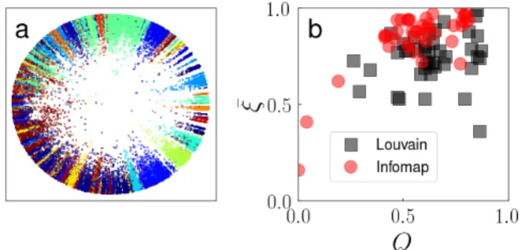
A direct comparison between the hyperbolic embedding and the community structure of the graphGconsists in a com-parison between the coordinates of the individual nodes in the two representations. Further, as the degree of the nodes triv-ially matches in both representations, the comparison reduces only in matching angular coordinatesθs and group member-shipsσs. From the numerous empirical tests we conducted on both real and synthetic networks, two main conclusions emerge. First, networks usually considered in hyperbolic em-bedding applications are highly modular, in the sense that par-titions found by community detection algorithms correspond to very large values of the modularity function Q[27] (see Figure1and SM. Second, nodes within the same communi-ties are likely to have similar angular coordinates. We note that this second finding is in line with what already shown in Ref. [16]. To quantify coherence among angular coordinates of nodes within the same communityg, we first define the variablesξgandφgwith
ξgeiφg = 1 ng N X j=1 δσj,ge iθj. (1)
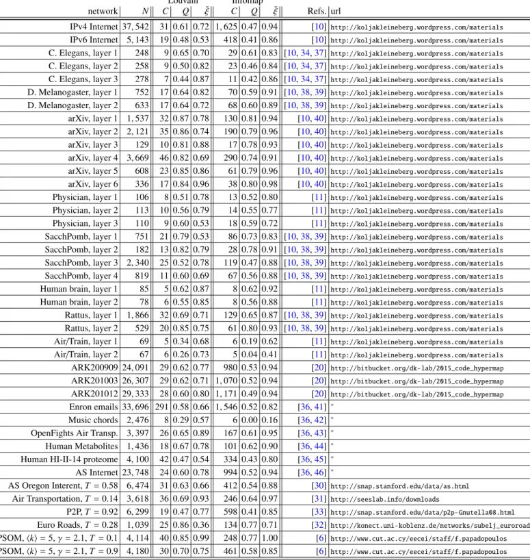
Figure 1. Hyperbolic embedding and community structure for real and synthetic networks. (a) We compare the hyperbolic embedding of the IPv4 Internet with its community structure. Every point rep-resents a node in the largest connected component of the graph. Po-sitions are determined by the radial and angular coordinates of the
nodes in the hyperbolic embedding of the network [10]. We use the
best partition found by the Louvain algorithm to determine the
com-munity structure of the graph [24]. The partition consists ofC=31
communities. Colors of the points identify community memberships.
The value of the modularity isQ=0.61, while angular coherence is
¯
ξ=0.72. (b) We consider 39 real-world networks and 2 instances
of the PSOM, and compare their community structure and hyper-bolic embedding (see details in SM). The plot displays each network
on the (Q,ξ)-plane. We show results obtained using Louvain (black¯
squares) and Infomap (red circles) [25].
δx,y=1 ifx=yandδx,y=0, otherwise. The r.h.s. of Eq. (1)
stands for the sums of vectors in the complex plane of the type eiθ =cos(θ)+i sin(θ) of all nodes in groupg. The vectorial
sum is divided by the community sizeng to obtain an
aver-age vector for the community.φgis the angular coordinate of
communityg. The module 0≤ξg ≤ 1 indicates how
coher-ent are the angular coordinates of the nodes within groupg. Note that the definition of Eq. (1) resembles the one used for the order parameter of the Kuramoto model [28]. We finally measure the angular coherence of a partition as the weighted average ¯ ξ= 1 N C X g=1 ngξg. (2)
By definition, we have that 0 ≤ ξ¯ ≤ 1. For all networks considered in our analysis (see Figure 1 and SM), angular coherence is typically large.
Our empirical tests demonstrate that strong angular coher-ence within communities of strongly modular networks is a quite robust feature of both synthetic and real systems. This finding tells us that the analogy between community structure and hyperbolic embedding may extend beyond the mere simi-larity among their ingredients. The following examples show that the analogy is useful also in the interpretation of physical properties of networks and the design of practical algorithms on networks.
Our first example regards the rephrasing, in terms of com-munity structure only, of a result obtained by analyzing the hyperbolic embedding of multiplex networks. In two recent
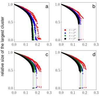
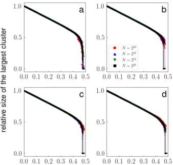
papers [10,11], Kleineberg and collaborators found that inter-layer correlation between hyperbolic coordinates of nodes in multiplex networks is a good predictor for the robustness of a system under targeted attack. Specifically, they found that, when correlation among angular coordinates is high, the per-colation transition is smooth. Instead, multiplex networks characterized by a small value of inter-layer correlation ex-hibit abrupt percolation transitions. The finding was initially obtained for real-world multiplex networks. A theoretical explanation was then given in terms of a synthetic network model [11]. To further support the analogy between hyper-bolic embedding and community structure that we are arguing for in this paper, we replicated all results of Ref. [11] using community structure only. First, we analyzed the same real-world multiplex networks considered in Ref. [11]. We found that their robustness can be predicted very well by the level of correlation among the community structures of the layers (see SM). Then, we provided a theoretical explanation. We replaced the network model by Kleineberget al. with a vari-ant of the SBM known in the literature as the Lancichinetti-Fortunato-Radicchi (LFR) benchmark graph [29]. The LFR model mostly differs from the standard SBM for relying on heterogeneous distributions of node degrees and community sizes. In our model for multiplex networks (see SM), we first generate a single LFR graph that is used as the topology for both layers. We then exchange the node labels in one layer to destroy edge overlap and degree-degree correlation. We con-sider two distinct scenarios. In the first case, we exchange the label of every node with the one of a randomly chosen node from the same community. This allows us to maintain per-fect correlation between the community structure of the two layers. In the second case, we exchange the labels of a num-ber of randomly sampled nodes such that the edge overlap between the layers equals the value obtained in the first ran-domization scheme. This second recipe completely destroys correlation between the community structures of the two lay-ers. In Fig.2a, we show the phase diagrams for instances of the multiplex model when relabeling uses information about the community structure of the graph. Here, the community structure is strong, in the sense that the fraction of external connections per node is onlyµ=0.1. The transition appears smooth, and becomes smoother as the size of the model in-creases. This is an indication that, in the limit of infinitely large LFR graphs, the percolation transition is likely continu-ous. In Fig.2b, we consider the second relabeling scheme that doesn’t account for community structure. The resulting dia-grams indicate that the percolation transition is abrupt. The level of correlation among community structure of the two layers can be decreased by increasingµ, so that community structure itself becomes less neat. This is done in Figs.2c and d, where the transition appear abrupt no matter how the labels of the nodes are relabeled. In SM, we report results for diff er-ent parameter values of the LFR model. Results confirm our claim that the extent of correlation between the community structure of the layers of a multiplex can be used to explain
Figure 2. Robustness of multiplex networks with correlated com-munity structure. We measure the relative size of the largest mutu-ally connected cluster as a function of the fraction of nodes removed from the system. The synthetic multiplex graphs are obtained using the recipe described in the text, where two
Lancichinetti-Fortunato-Radicchi (LFR) networks with sizeNare coupled together. The LFR
models are such that: the average degree ishki=6; the maximum
degree iskmax=
√
N; node degreeskobey a power-law distribution P(k) ∼ k−γ
with exponentγ = 2.6; there areC =
√
N
communi-ties of identical sizeS = √N. For everyN, we show the results
for five distinct instances of the model. (a) LFR graphs are
gener-ated withµ=0.1. Labels are exchanged only among nodes within
the same clusters. All nodes are considered for relabeling at least once. (b) Same as in panel a. However, relabeling of nodes is not constrained by community structure. The number of nodes that are relabeled is such that the edge overlap among layers is the same as in panel a (SM). (c and d) Same as in panels a and b, respectively, but
for LFR graphs constructed usingµ=0.3.
robustness properties of the system under targeted attack.
Our second example focuses on greedy routing [2,7]. To be brief, the scenario considered is the following. A packet originated by nodesmust be delivered to nodet. The packet can navigate the network by walking at each step on an edge. The packet moves on the network till it reaches its destination t, or it visits twice the same node. In the first case, the packet is correctly delivered. In the second case, the packet is con-sidered lost, and it is discarded. The goal of a good routing strategy is to deliver packets with high probability and with a small number of steps, for any randomly chosen pair of source and target nodessandt. Hyperbolic embedding turns out to be very useful in the formulation of a greedy strategy, where individual steps are determined on the basis of the distance among nodes in the hyperbolic space. Specifically, if a
mes-sage is at nodei, then the next move will be on the node
j(best)(i) =arg min
j∈Ni
d(j,t), (3) whereNiis the set of neighbors ofi, andd(j,t) is the distance
between nodes jandt. The greedy technique is computation-ally feasible as every node needs to know only the identity and the geometric coordinates of its neighbors. The regimes of effectiveness of the routing method have been systemati-cally studied in artificial network models [2]. The technique has been proven to be extremely effective on some real-world topologies [2,7]. We devised a new greedy routing protocol that makes use of the cluster structure of a network instead of its hyperbolic embedding. Specifically, we replaced the defi-nition of distance in the hyperbolic space between nodes with the fitness
d(j,t)=βDσj,σt−(1−β) lnkj, (4)
wherekjis the degree of node j, andσjandσtare the indices
of the communities of nodesjandt, respectively.Dσj,σtis the
length of the shortest path between communities σj andσt
calculated on a weighted supernetwork in which supernodes are communities of the original network. Each pair of su-pernodesgandqis connected with a superedge with weight
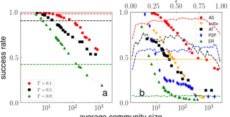
Figure 3. Performance of community-based routing. (a) We
con-sider single instances of the growing network model of Ref. [21]
withN =5,000 nodes,hki=5, and degree exponentγ=2.1.
Dif-ferent symbols and colors refer to different values of the temperature
T. The plot shows how success rate of the community-based greedy
routing strategy changes as a function the average size of the com-munities. Communities are identified using the algorithm by
Ron-hovde and Nussinov [26]. Their number can be varied by changing
the resolution level of the algorithm. Dashed lines are obtained on the same networks but using hyperbolic greedy routing. (b) Same as in panel a, but for real networks. We consider the following
net-works: the Internet at the level of autonomous systems (AS) [30]; the
worldwide air transportation network (AT) [31]; the European road
network (ER) [32]; the peer-to-peer network (P2P) [33]; the arXiv
collaboration network [34]. For all the networks (except arXiv) the
dashed lines are obtained by varying the temperatureT in the
algo-rithm for hyperbolic embedding introduced in Ref. [20]; for the arXiv
network the dashed line shows the result for the optimum hyperbolic
coordinates whose data was available in [10]. Details can be found
in SM.
1−lnρg,q; hereρg,qis the probability that, in the original
net-work, a randomly chosen node in communityghas an edge to communityq(see SM). The term lnkjin Eq. (4) serves to
perform degree correction. The factor 0 ≤ β ≤ 1 serves to control the relative importance of one factor over the other.β plays a similar role as of the temperatureTin hyperbolic rout-ing protocols [20], and its value may be appropriately chosen with the goal of optimizing the success rate in the delivery of messages (see SM). The routing protocol based on Eq. (4) is still computationally efficient as long as the total number of communitiesCgrows sub-linearly with the size of the graph N. In the extreme case, where every community is formed by a single node, so thatC =N, the method will be 100% accu-rate in delivering packets, but also computationally expensive. In Figure3, we display the performance of community-based greedy routing as a function of the mean size of the com-munities. We study the performance on both synthetic and real-world networks. The number of communities is tuned by changing the resolution parameter in the algorithm by Ron-hovde and Nussinov [26]. Success rates of the community-based greedy protocol are always very good, as long as com-munities are not too large.
In summary, we showed that looking at a network as em-bedded in a hyperbolic geometry is similar, both in theory and practice, to pretending that the network is organized into communities, provided that community structure is detected by a method that accounts for the degree of the nodes. Our finding provides evidence that the inter-community structure in networks may have geometric organization, meaning that at the global level, geometry dominates, while at the local scale, community memberships prevail. Thus, real networks may be modeled by a graphon [35] consisting of a mixture of latent-spatial and block-like structures. This fundamental model has the potential to generate further understanding of physical processes, such as spreading and synchronization, in real networks.
The authors thank G. Bianconi, C. V. Cannistraci, D. Kri-oukov , and M. ´A. Serrano for comments on the manuscript. A.F. and F.R. acknowledge support from the U.S. Army Re-search Office (W911NF-16-1-0104). F.R. acknowledges sup-port from the National Science Foundation (CMMI-1552487). A.F. acknowledges support from the Science Foundation Ire-land (16/IA/4470).
SUPPLEMENTAL MATERIAL Hyperbolic embedding and community detection
In tableS1, we provide a list of all networks considered in our analysis.
We obtain hyperbolic coordinates of networks in the fol-lowing way. For real networks, we either rely on embed-dings publicly available [10,20] or we apply publicly avail-able algorithms to the graphs [20]. Urls of electronic re-sources for all networks are provided in tableS1. In the hy-perbolic embeddings that we performed, we made use of the algorithm provided inhttps://bitbucket.org/dk-lab/ 2015_code_hypermap. As prescribed in Ref. [20], the value of the temperatureT used in the embedding corresponds to the one leading to maximal success rate in greedy routing [2,7] (see section below). We further consider two instances of the popularity-similarity optimization model (PSOM) [6]. They are generated using different values of the model pa-rameters. The code to generate instances of the PSOM has been taken fromhttps://www.cut.ac.cy/eecei/staff/ f.papadopoulos.
We use three distinct methods for detecting communi-ties in networks: the Louvain algorithm [24], Infomap [25], and the algorithm by Ronhovde and Nussinov [26]. Lou-vain and Infomap are used in the analysis about the rela-tion between hyperbolic embedding and community struc-ture (see TableS1). The algorithm by Ronhovde and Nussi-nov is used in the analysis of greedy routing. For Lou-vain and Infomap we rely on the algorithms implemented in the library http://igraph.org/python. We consider always the “best” (i.e., the one with maximum modularity for Louvain , the one with minimum description length for Infomap) partitions found by the algorithms. The imple-mentation of the algorithm by Ronhovde and Nussinov was taken from http://www.elemartelot.org/index.php/ programming/cd-code. We chose this algorithm to study greedy routing as it allows for a finer tuning of the resolution of the community structure than the other two algorithms. Af-ter obtaining the modular structure from this algorithm, we perform an additional step to improve the quality of commu-nities: If there is any community with size one we change the community label of the only member of that community to the label of its highest degree neighbor.
Community structure and robustness of real-world multiplex networks
We performed the same type of analysis as in Ref. [11] by studying the relation between system robustness and “ge-ometric” correlations among the network layers in real multi-plex networks. We just replaced hyperbolic embedding with community structure. Specifically, given a multiplex network composed of two layers, we first detect communities in the largest connected component of both layers independently by
using either Louvain or Infomap. Correlation between the community structure of the layers is measured using the nor-malized mutual information (NMI) defined in Ref. [47]. As the number of nodes in the layers may be different, in the computation of the NMI values, we considered only nodes appearing in both layers. We finally used the obtained NMI values in the scatter plots of Fig.S1. We find that the robust-ness of the various networks can be predicted equally well by looking at correlations among either hyperbolic coordinates or community memberships of the nodes in the two layers (see panels a–c). Further, we find that NMI values in the various representations are strongly correlated (panels d–e).
Multiplex networks with correlated community structure
The first step in the creation of a single instance of our multiplex model consists in generating a single instance of the Lancichinetti-Fortunato-Radicchi (LFR) model [29]. The LFR model is a variant of the degree-corrected stochastic block model. The model allows to generate single-layer net-works with built-in community structure, where both the de-gree distributionP(k) and community size distributionP(S) are power-law functions, i.e., P(k) ∼ k−γ and P(S) ∼ S−β. In addition to the exponentsγandβ, in the generation of one instance of the LFR model, one needs to specify the value of several parameters, including: average degreehki, maxi-mum degreekmax, minimumsminand maximumsmax
commu-nity size, size of the networkN, and the mixing parameter
µ. The mixing parameter 0 ≤ µ ≤ 1 specifies the fraction of edges that a single node shares with nodes outside its own community. This parameter plays a fundamental role to deter-mine how strong the community structure is. Low values ofµ correspond to a strong community structure. Asµincreases, community structure becomes fuzzy. The maximal value of
µfor which planted community structure is exactly recover-able is bounded by a quantity calculated in Ref. [48]. In our simulations, we useµ = 0.1 to represent a regime of strong community structure, andµ =0.3 for regime of loose com-munity structure. These values have been chosen arbitrarily, thinking to the application of the model here. For example, we didn’t useµvalues too close to zero to avoid the presence of disconnected components.
Once a single instance of the LFR model is generated, we use that instance to define the topology of both layers of the multiplex. Node labels of the two layers are initially identical, so that the adjacency matrices of the two layers are identical. We then start relabeling nodes of one layer only. As already mentioned in the main text, we use two different strategies for relabeling. In the first strategy, we make use of the known community structure. In essence, in the relabeling procedure, the label of every node is exchanged with the one of another node randomly chosen from the same community. In the other procedure instead, the constraint on the group memberships is not used. This second variant corresponds to the same model already considered in Refs. [49,50]. In this second variant,
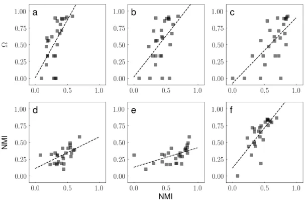
Figure S1. Community structure and robustness of real multiplex networks. We consider the 26 multiplex networks analyzed in Ref. [11]. As
in Ref. [11], we rely on the quantityΩas a proxy to evaluate the robustness of a given multiplex network. Ω =(∆N−∆Nrs)/(∆N+ ∆Nrs),
where∆Nand∆Nrsare respectively the widow sizes of the transitions in targeted and random percolation processes on the network.Ωvalues
for the various networks have been taken from the supplemental material of Ref. [11]. The normalized mutual information (NMI) serves to
quantify similarity between the embedding of the nodes in the two layers. Values of the NMI for hyperbolic embedding have also been taken
from the supplemental material of Ref. [11]. We calculated instead NMI values among the community structures found for the layers of a
multiplex using the definition provided in Ref. [47]. Communities in each layer are found using either Louvain or Infomap. (a) As a reference,
we reproduced the same plot as in Fig. 4 of Ref. [11], where each network represents a point in the (NMI,Ω)-plane. The dashed line is
obtained with simple linear regression. The correlation coefficient calculated from the data points isr =0.63. (b) Same as in panel a, but
for NMI values calculated using the community structures found by the Louvain algorithm. Herer =0.54. (c) Same as in panel b, but for
NMI values calculated using the community structures found by Infomap. We measuredr=0.68 in this case. (d, e, and f) We compare NMI
values obtained using the various embedding methods. The various panels represent: (d) Louvainvs. hyperbolic (r=0.56); (e) Infomapvs.
hyperbolic (r=0.55); (f) Infomapvs.Louvain (r=0.76).
we perform a number of label swaps such that the value of the edge overlap among the two layers is comparable with the one obtained in the first variant of the model. Both variants of the multiplex model essentially lead to very small values of edge overlap and degree-degree correlation between layers. The first variant, however, preserves perfect correlation between the community structure of the two layers, while the second variant destroys it completely.
The robustness of single instances of the multiplex model described above are then studied as in Ref. [11]. Every node iin the network has associated the scoreKi =max (k(1)i ,k(2)I ),
withki(x)the degree of nodeiin layerx. Nodes are then ranked in descending order according to this score, with ties ran-domly broken. The top node is removed from the network. After every removal, the score is Ki of every node istill in
the system is recomputed. Further, the relative size of the mu-tually connected giant component is evaluated to construct a percolation phase diagram [51].
We considered various sets of parameters for the genera-tion of the LFR model. All of them provide the same type of message. When the community structure is strong (i.e., small
µvalues), the model with correlated community structure un-dergoes a smooth percolation transition. If correlation in com-munity structure is destroyed, the transition becomes abrupt. If the community structure is not strong (i.e., largeµvalues), then both relabeling schemes lead to an abrupt transition. The result is valid also for LFR models with homogenous degree distribution (see FigureS2).
Greedy routing
As already considered in Refs. [2,7], we immagine that a packet is traveling from the source nodesto the target node t in a network withN nodes and adjacency matrix A. The packet moves on edges of the network, performing a single
Table S1. Relation between community structure and hyperbolic embedding in real and synthetic networks. From left to right, we report:
name of the network, size of the giant componentN, number of communitiesCidentified by the Louvain algorithm, value of the modularityQ
corresponding to the Louvain partition, angular coherence ¯ξof the Louvain partition, number of communitiesCidentified by Infomap, value
of the modularityQcorresponding to the Infomap partition, angular coherence ¯ξof the Infomap partition, reference(s) of the papers where
the dataset was reported and/or where hyperbolic coordinates of the network were obtained, urls of the websites where the corresponding data
can be downloaded. If the url is denoted by∗
, this means that data were obtained from a private communication and they are available upon request from the authors of Ref. [36].
Louvain Infomap
network N C Q ξ¯ C Q ξ¯ Refs. url
IPv4 Internet 37,542 31 0.61 0.72 1,625 0.47 0.94 [10] http://koljakleineberg.wordpress.com/materials
IPv6 Internet 5,143 19 0.48 0.53 418 0.41 0.86 [10] http://koljakleineberg.wordpress.com/materials
C. Elegans, layer 1 248 9 0.65 0.70 29 0.61 0.83 [10,34,37] http://koljakleineberg.wordpress.com/materials
C. Elegans, layer 2 258 9 0.50 0.82 23 0.46 0.84 [10,34,37] http://koljakleineberg.wordpress.com/materials
C. Elegans, layer 3 278 7 0.44 0.87 11 0.42 0.86 [10,34,37] http://koljakleineberg.wordpress.com/materials
D. Melanogaster, layer 1 752 17 0.64 0.82 70 0.59 0.91 [10,38,39] http://koljakleineberg.wordpress.com/materials
D. Melanogaster, layer 2 633 17 0.64 0.72 68 0.60 0.89 [10,38,39] http://koljakleineberg.wordpress.com/materials
arXiv, layer 1 1,537 32 0.87 0.78 130 0.81 0.94 [10,40] http://koljakleineberg.wordpress.com/materials
arXiv, layer 2 2,121 35 0.86 0.74 190 0.79 0.96 [10,40] http://koljakleineberg.wordpress.com/materials
arXiv, layer 3 129 10 0.81 0.88 17 0.78 0.93 [10,40] http://koljakleineberg.wordpress.com/materials
arXiv, layer 4 3,669 46 0.82 0.69 290 0.74 0.91 [10,40] http://koljakleineberg.wordpress.com/materials
arXiv, layer 5 608 23 0.85 0.86 61 0.79 0.96 [10,40] http://koljakleineberg.wordpress.com/materials
arXiv, layer 6 336 17 0.84 0.96 38 0.80 0.98 [10,40] http://koljakleineberg.wordpress.com/materials
Physician, layer 1 106 8 0.51 0.78 13 0.52 0.80 [11] http://koljakleineberg.wordpress.com/materials
Physician, layer 2 113 10 0.56 0.79 14 0.55 0.77 [11] http://koljakleineberg.wordpress.com/materials
Physician, layer 3 110 9 0.60 0.53 18 0.59 0.72 [11] http://koljakleineberg.wordpress.com/materials
SacchPomb, layer 1 751 21 0.79 0.53 86 0.73 0.83 [10,38,39] http://koljakleineberg.wordpress.com/materials
SacchPomb, layer 2 182 13 0.82 0.79 28 0.78 0.91 [10,38,39] http://koljakleineberg.wordpress.com/materials
SacchPomb, layer 3 2,340 25 0.52 0.78 119 0.47 0.88 [10,38,39] http://koljakleineberg.wordpress.com/materials
SacchPomb, layer 4 819 11 0.60 0.69 67 0.56 0.88 [10,38,39] http://koljakleineberg.wordpress.com/materials
Human brain, layer 1 85 5 0.62 0.87 8 0.62 0.92 [11] http://koljakleineberg.wordpress.com/materials
Human brain, layer 2 78 6 0.55 0.85 8 0.56 0.88 [11] http://koljakleineberg.wordpress.com/materials
Rattus, layer 1 1,866 32 0.69 0.71 129 0.65 0.87 [10,38,39] http://koljakleineberg.wordpress.com/materials
Rattus, layer 2 529 20 0.85 0.75 61 0.80 0.93 [10,38,39] http://koljakleineberg.wordpress.com/materials
Air/Train, layer 1 69 5 0.34 0.68 6 0.19 0.62 [11] http://koljakleineberg.wordpress.com/materials
Air/Train, layer 2 67 6 0.26 0.73 5 0.04 0.41 [11] http://koljakleineberg.wordpress.com/materials
ARK200909 24,091 29 0.62 0.77 980 0.53 0.94 [20] http://bitbucket.org/dk-lab/2015_code_hypermap
ARK201003 26,307 29 0.62 0.71 1,070 0.52 0.94 [20] http://bitbucket.org/dk-lab/2015_code_hypermap
ARK201012 29,333 28 0.60 0.80 1,171 0.49 0.94 [20] http://bitbucket.org/dk-lab/2015_code_hypermap
Enron emails 33,696 291 0.58 0.66 1,546 0.52 0.82 [36,41] ∗
Music chords 2,476 8 0.29 0.57 6 0.00 0.16 [36,42] ∗
OpenFights Air Transp. 3,397 26 0.65 0.89 167 0.61 0.95 [36,43] ∗
Human Metabolites 1,436 18 0.67 0.78 101 0.62 0.90 [36,44] ∗
Human HI-II-14 proteome 4,100 42 0.47 0.54 334 0.43 0.80 [36,45] ∗
AS Internet 23,748 24 0.60 0.78 994 0.52 0.94 [36,46] ∗
AS Oregon Interent,T =0.58 6,474 31 0.63 0.66 412 0.54 0.88 [30] http://snap.stanford.edu/data/as.html
Air Transportation,T =0.14 3,618 36 0.69 0.93 246 0.64 0.97 [31] http://seeslab.info/downloads
P2P,T =0.92 6,299 19 0.47 0.77 598 0.41 0.85 [33] http://snap.stanford.edu/data/p2p-Gnutella08.html
Euro Roads,T =0.28 1,039 25 0.86 0.36 134 0.77 0.71 [32] http://konect.uni-koblenz.de/networks/subelj_euroroad
PSOM,hki=5,γ=2.1,T =0.1 4,114 40 0.85 0.99 248 0.77 1.00 [6] http://www.cut.ac.cy/eecei/staff/f.papadopoulos
hop at each stage of the dynamics. Greedy routing relies on a definition of “distance” between pairs of nodes in the net-work. At every stager of the dynamics towards the target nodet, a packet sitting on nodepr =ichoose to move to the
node j(best)(i) defined in Eq. (4) of the main text. In essence, j(best)(i) is the neighbor of nodeithat has minimal distance to the target node t. In our numerical simulations, we avoid immediate backtracking walks of the packet, therefore node j(best)(i) = pr+1 , pr−1, i.e., cannot be equal to the node
vis-ited before nodei; this condition improves significantly (not shown) the performance of both methods considered in this paper. The packet continues to travel until one of these two conditions is met: (i) the packet arrives at destination afterR steps, i.e., pR =t; (ii) the packet visits twice the same node,
i.e.,pr=pv, withv<r. Condition (i) corresponds to success.
Condition (ii) represents failure and the packet is discarded. To evaluate performance of the routing protocol, we use at leastB=10,000 numerical simulations. In each simulation,
Figure S2. Robustness of multiplex networks with correlated com-munity structure. We measure the relative size of the largest mutu-ally connected cluster as a function of the fraction of nodes removed from the system. The synthetic multiplex graphs were obtained using the recipe described in the text, where two
Lancichinetti-Fortunato-Radicchi (LFR) models with sizeNare coupled together. The LFR
models are such that: the average degree ishki=6 and the maximum
degree iskmax=6, so that degree of all nodes isk=6; communities
have identical sizeS =64. For every value ofNwe show the results
for five distinct instances of the model. (a) LFR graphs are generated
withµ = 0.1. Labels are exchanged only among nodes within the
same clusters. (b) Same as in panel a. However, relabeling of nodes is allowed among all nodes in the network. Probabilities of relabel-ing in panels a and b are such that the edge overlap among layers is the same for both models. (c and d) Same as in panels a and b,
respectively, but for LFR graphs constructed usingµ=0.3.
Figure S3. Same analysis as in Figure 3 of the main text.
Perfor-mance is measured in terms of efficiency (panels a and b), and the
average path length of successfully delivered packets (panels c and d).
sourcesand target t nodes are randomly chosen among the nodes in the giant connected component of the network. We quantify three different metrics of performance:
1) The success ratez, i.e., the fraction of packets correctly delivered. This is a metric of performance introduced in Ref. [2]. Results for this metric are presented in Fig-ure 3 of the main text.
2) The average value ofhRi, i.e., the average length of the paths for successfully delivered packets. This metric of performance was also introduced in Ref. [2]. Results for this metric are presented in FiguresS3c and d.
3) Efficiency η = zh1/Ri, where h1/Ri represents the mean value of the inverse of the path length obtained for each of the successfully delivered packets. This def-inition ofηis based on a metric of performance intro-duced in Ref. [23]. Results for this metric are presented in FiguresS3a and b.
It is worth noting that the efficiency measure (which is a bal-ance between success rate and path length) shows similar re-sults as those of the success rate (FigureS3a and b); this is because for almost all the networks of FigureS3, the path length does not change remarkably as the mean community size or the temperature is altered (FiguresS3c and d). Thus, the success rate results (investigated in Figure 3 of the main text) are sufficient to assess the performance of the two routing methods investigated in this paper.
In the standard application of network hyperbolic embed-ding, the distance between pairs of nodes is given by their dis-tance in the hyperbolic space [2,7]. In our community-based routing protocol, we substituted the distance in the hyperbolic space with the analogous quantity based on thea priorigiven community structure of the graph. Specifically, we define the weight between the connected modulesgandqas
wg,q=1−lnρg,q , ifρg,q>0, (S1) where ρg,q= P i>jAi,jδσi,gδσj,q P i>jAi,jδσi,g . (S2)
In the above equation,δx,y =1, ifx=y, whileδx,y =0,
oth-erwise; Ai,j = Aj,i = 1 if nodesiand jare connected, while
Ai,j=Aj,i=0, otherwise;σiis the group membership of node
iaccording to the given community structure. Eq. (S2) is the ratio between the total number of edges shared between nodes within communitiesgandq, and the total degree of nodes in communityg. ρg,qcan be also interpreted as the probability
that following a random edge of a random node in moduleg we reach a node in moduleq. We consider each community as a supernode, and the network as a supernetwork composed of supernodes connected with weighted superedges. The weight of the superedge between supernodes g andq is defined in Eq. (S1). Then, we find the length of the shortest paths be-tween every pair of supernodes. This operation relies on the algorithm by Johnson [52]. The output is a full matrixDthat includes the distances between every pair of modules. The generic elementDg,qof this matrix contains a sum of weights
defined in Eq. (S1), which is basically equivalent to a sort of expected path length between communitiesgandq, under the hypothesis that connections were generated according to the stochastic block model [12]. Given that we are at node iat stagerof the trajectory of the packet, the “distance” between
Figure S4. Same analysis as in Figure 3 of the main text. For each
modular structure theβvalue for which we obtained the highest
suc-cess rate is reported.
a neighbor jof nodeiand the targettis finally defined as
dj,t=βDσj,σt +(1−β)nh1−logkjρσi,σj i −h1−logρσi,σj io (S3) =βDσj,σt−(1−β) lnkj (S4)
wherekjis the degree of node j, and 0≤β≤1. The previous
expression defines a measure of “distance” between node j and moduleσt. This is computed as a distance between
mod-ulesσjandσt, but corrected for the fact that we are aware of
the degree of node j. This definition of distance is motivated by the degree-corrected stochastic block model in which the probability that following a randomly chosen edge from com-munityσjwe reach a node in communityσj0is proportional tokjρσj,σj0. Note that we are aware also of the degrees of nodesiandt, but this information is not helpful in the proto-col. The factorβserves to weight the importance of the com-munity structurevs. the degree of the individual nodes in the definition of distance. This factor can be tuned appropriately to optimize the success rate of the greedy routing protocol. Optimal values used in our simulations are displayed in Fig-ureS4. As FigureS4illustrates, the most optimum value of
βdepends on the network structure and also on the consid-ered modular structure; more specifically,βis more likely to be close to 1 for networks with lower temperatures (or eff ec-tively those with higher clustering coefficients) and for modu-lar structures with smaller mean community sizes.
[1] M Angeles Serrano, Dmitri Krioukov, and Mari´an
Bo-gun´a, “Self-similarity of complex networks and hidden metric
spaces,” Physical Review Letters100, 078701 (2008).
[2] Marian Boguna, Dmitri Krioukov, and Kimberly C Claffy,
“Navigability of complex networks,” Nature Physics5, 74–80
(2009).
[3] Dmitri Krioukov, Fragkiskos Papadopoulos, Amin Vahdat, and Mari´an Bogun´a, “Curvature and temperature of complex
net-works,” Physical Review E80, 035101 (2009).
[4] Dmitri Krioukov, Fragkiskos Papadopoulos, Maksim Kitsak, Amin Vahdat, and Mari´an Bogun´a, “Hyperbolic geometry of
complex networks,” Physical Review E82, 036106 (2010).
[5] Ginestra Bianconi and Christoph Rahmede, “Emergent
hyper-bolic network geometry,” Scientific Reports7(2017).
[6] Fragkiskos Papadopoulos, Maksim Kitsak, M ´Angeles Serrano,
Mari´an Bogun´a, and Dmitri Krioukov, “Popularity versus
sim-ilarity in growing networks,” Nature489, 537–540 (2012).
[7] Mari´an Bogun´a, Fragkiskos Papadopoulos, and Dmitri Kri-oukov, “Sustaining the internet with hyperbolic mapping,”
Na-ture Communications1, 62 (2010).
[8] M ´Angeles Serrano, Mari´an Bogu˜n´a, and Francesc Sagu´es,
“Uncovering the hidden geometry behind metabolic networks,”
Molecular BioSystems8, 843–850 (2012).
[9] Guillermo Garc´ıa-P´erez, Mari´an Bogu˜n´a, Antoine Allard, and
M ´Angeles Serrano, “The hidden hyperbolic geometry of
inter-national trade: World trade atlas 1870–2013,” Scientific reports
[10] Kaj-Kolja Kleineberg, Mari´an Bogun´a, M ´Angeles Serrano, and Fragkiskos Papadopoulos, “Hidden geometric correlations
in real multiplex networks,” Nature Physics 12, 1076–1081
(2016).
[11] Kaj-Kolja Kleineberg, Lubos Buzna, Fragkiskos Papadopoulos,
Mari´an Bogu˜n´a, and M ´Angeles Serrano, “Geometric
correla-tions mitigate the extreme vulnerability of multiplex networks
against targeted attacks,” Physical Review Letters118, 218301
(2017).
[12] Brian Karrer and Mark EJ Newman, “Stochastic blockmodels
and community structure in networks,” Physical Review E83,
016107 (2011).
[13] Santo Fortunato, “Community detection in graphs,” Physics
re-ports486, 75–174 (2010).
[14] Tiago P Peixoto, “Bayesian stochastic blockmodeling,” arXiv preprint arXiv:1705.10225 (2017).
[15] MEJ Newman, “Equivalence between modularity optimization and maximum likelihood methods for community detection,”
Physical Review E94, 052315 (2016).
[16] Zuxi Wang, Qingguang Li, Fengdong Jin, Wei Xiong, and Yao Wu, “Hyperbolic mapping of complex networks based on com-munity information,” Physica A: Statistical Mechanics and its
Applications455, 104–119 (2016).
[17] Konstantin Zuev, Mari´an Bogu˜n´a, Ginestra Bianconi, and
Dmitri Krioukov, “Emergence of soft communities from
ge-ometric preferential attachment,” Scientific reports 5, 9421
(2015).
[18] Guillermo Garc´ıa-P´erez, M. ´Angeles Serrano, and Mari´an
Bogu˜n´a, “Soft communities in similarity space,” Journal of Sta-tistical Physics (2018).
[19] Alessandro Muscoloni and Carlo Vittorio Cannistraci, “A nonuniform popularity-similarity optimization (npso) model to
efficiently generate realistic complex networks with
communi-ties,” arXiv preprint arXiv:1707.07325 (2017).
[20] Fragkiskos Papadopoulos, Rodrigo Aldecoa, and Dmitri Kri-oukov, “Network geometry inference using common
neigh-bors,” Physical Review E92, 022807 (2015).
[21] Fragkiskos Papadopoulos, Constantinos Psomas, and Dmitri Krioukov, “Network mapping by replaying hyperbolic growth,”
IEEE/ACM Transactions on Networking (TON) 23, 198–211
(2015).
[22] Gregorio Alanis-Lobato, Pablo Mier, and Miguel A
Andrade-Navarro, “Efficient embedding of complex networks to
hyper-bolic space via their laplacian,” Scientific reports 6, 30108
(2016).
[23] Alessandro Muscoloni, Josephine Maria Thomas, Sara Ciucci, Ginestra Bianconi, and Carlo Vittorio Cannistraci, “Machine learning meets complex networks via coalescent embedding in
the hyperbolic space,” Nature Communications8, 1615 (2017).
[24] Vincent D Blondel, Jean-Loup Guillaume, Renaud Lambiotte, and Etienne Lefebvre, “Fast unfolding of communities in large networks,” Journal of statistical mechanics: theory and
experi-ment2008, P10008 (2008).
[25] Martin Rosvall and Carl T Bergstrom, “Maps of random walks on complex networks reveal community structure,” Proceedings
of the National Academy of Sciences105, 1118–1123 (2008).
[26] Peter Ronhovde and Zohar Nussinov, “Local
resolution-limit-free potts model for community detection,” Phys. Rev. E 81,
046114 (2010).
[27] Mark EJ Newman and Michelle Girvan, “Finding and
evaluat-ing community structure in networks,” Physical Review E69,
026113 (2004).
[28] Yoshiki Kuramoto,Chemical oscillations, waves, and
turbu-lence(Dover Publications, New York, 1984).
[29] Andrea Lancichinetti, Santo Fortunato, and Filippo
Radic-chi, “Benchmark graphs for testing community detection
algo-rithms,” Physical review E78, 046110 (2008).
[30] Jure Leskovec, Jon Kleinberg, and Christos Faloutsos, “Graphs over time: densification laws, shrinking diameters and possible
explanations,” inProceedings of the eleventh ACM SIGKDD
in-ternational conference on Knowledge discovery in data mining (ACM, 2005) pp. 177–187.
[31] R. Guimer`a, S. Mossa, A. Turtschi, and L. A. N. Amaral, “The worldwide air transportation network: Anomalous centrality, community structure, and cities’ global roles,” Proceedings of
the National Academy of Sciences102, 7794–7799 (2005).
[32] L. ˇSubelj and M. Bajec, “Robust network community detection using balanced propagation,” The European Physical Journal B
81, 353–362 (2011).
[33] Matei Ripeanu and Ian Foster, “Mapping the gnutella net-work: Macroscopic properties of large-scale peer-to-peer
sys-tems,” inPeer-to-Peer Systems, edited by Peter Druschel, Frans
Kaashoek, and Antony Rowstron (Springer Berlin Heidelberg, Berlin, Heidelberg, 2002) pp. 85–93.
[34] Manlio De Domenico, Mason A Porter, and Alex Arenas,
“Muxviz: a tool for multilayer analysis and visualization of
net-works,” Journal of Complex Networks3, 159–176 (2015).
[35] L´aszl´o Lov´asz, Large networks and graph limits, Vol. 60
(American Mathematical Soc., 2012).
[36] Guillermo Garz´ıa-P´erez, Marian Boguna, and Serrano M.
´
Angeles, “Multiscale unfolding of real networks by geometric
renormalization,” Nature Physics-, – (2018).
[37] Beth L Chen, David H Hall, and Dmitri B Chklovskii, “Wiring optimization can relate neuronal structure and function,” Pro-ceedings of the National Academy of Sciences of the United
States of America103, 4723–4728 (2006).
[38] Chris Stark, Bobby-Joe Breitkreutz, Teresa Reguly, Lorrie Boucher, Ashton Breitkreutz, and Mike Tyers, “Biogrid: a gen-eral repository for interaction datasets,” Nucleic acids research
34, D535–D539 (2006).
[39] Manlio De Domenico, Vincenzo Nicosia, Alexandre Arenas, and Vito Latora, “Structural reducibility of multilayer
net-works,” Nature communications6, 6864 (2015).
[40] Manlio De Domenico, Andrea Lancichinetti, Alex Arenas, and Martin Rosvall, “Identifying modular flows on multilayer networks reveals highly overlapping organization in
intercon-nected systems,” Physical Review X5, 011027 (2015).
[41] Jure Leskovec, Kevin J Lang, Anirban Dasgupta, and
Michael W Mahoney, “Community structure in large networks: Natural cluster sizes and the absence of large well-defined
clus-ters,” Internet Mathematics6, 29–123 (2009).
[42] Joan Serr`a, ´Alvaro Corral, Mari´an Bogu˜n´a, Mart´ın Haro, and
Josep Ll Arcos, “Measuring the evolution of contemporary
western popular music,” Scientific reports2, 521 (2012).
[43] J´erˆome Kunegis, “Konect: the koblenz network collection,” in Proceedings of the 22nd International Conference on World Wide Web(ACM, 2013) pp. 1343–1350.
[44] M ´Angeles Serrano, Mari´an Bogun´a, and Francesc Sagu´es,
“Uncovering the hidden geometry behind metabolic networks,”
Molecular biosystems8, 843–850 (2012).
[45] Thomas Rolland, Murat Tas¸an, Benoit Charloteaux, Samuel J Pevzner, Quan Zhong, Nidhi Sahni, Song Yi, Irma Lemmens,
Celia Fontanillo, Roberto Mosca, et al., “A proteome-scale
map of the human interactome network,” Cell159, 1212–1226
(2014).
[46] K. Claffy, Y. Hyun, K. Keys, M. Fomenkov, and D. Krioukov,
“Internet mapping: From art to science,” in2009
Secu-rity(2009) pp. 205–211.
[47] Leon Danon, Albert Diaz-Guilera, Jordi Duch, and Alex Are-nas, “Comparing community structure identification,” Journal
of Statistical Mechanics: Theory and Experiment2005, P09008
(2005).
[48] Filippo Radicchi, “Decoding communities in networks,” Phys.
Rev. E97, 022316 (2018).
[49] Filippo Radicchi, “Percolation in real interdependent
net-works,” Nature Physics11, 597 (2015).
[50] Saeed Osat, Ali Faqeeh, and Filippo Radicchi, “Optimal
perco-lation on multiplex networks,” Nature Communications8, 1540
(2017).
[51] Sergey V Buldyrev, Roni Parshani, Gerald Paul, H Eugene Stanley, and Shlomo Havlin, “Catastrophic cascade of failures
in interdependent networks,” Nature464, 1025 (2010).
[52] Donald B Johnson, “Efficient algorithms for shortest paths in