Deep learning models of biological visual information processing

(1)

biological visual information processing. PhD thesis,

University of Nottingham.

Access from the University of Nottingham repository:

http://eprints.nottingham.ac.uk/35561/1/thesis_DianaTurcsany.pdf Copyright and reuse:

The Nottingham ePrints service makes this work by researchers of the University of Nottingham available open access under the following conditions.

This article is made available under the University of Nottingham End User licence and may be reused according to the conditions of the licence. For more details see:

http://eprints.nottingham.ac.uk/end_user_agreement.pdf

(2)

The University of Nottingham

School of Computer Science

Deep Learning Models of Biological

Visual Information Processing

Diána Turcsány

Thesis submitted to The University of Nottingham

for the degree of Doctor of Philosophy

(3)

Abstract

Improved computational models of biological vision can shed light on key processes contributing to the high accuracy of the human visual system. Deep learning models, which extract multiple layers of increasingly complex features from data, achieved recent breakthroughs on visual tasks. This thesis proposes such flexible data-driven models of biological vision and also shows how insights regarding biological visual processing can lead to advances within deep learning. To harness the potential of deep learning for modelling the retina and early vision, this work introduces a new dataset and a task simulating an early visual processing function and evaluates deep belief networks (DBNs) and deep neural networks (DNNs) on this input. The models are shown to learn feature detectors similar to retinal ganglion and V1 simple cells and execute early vision tasks.

To model high-level visual information processing, this thesis proposes novel deep learning architectures and training methods. Biologically inspired Gaussian receptive field constraints are imposed on restricted Boltzmann machines (RBMs) to improve the fidelity of the data representation to encodings extracted by visual processing neurons. Moreover, concurrently with learning local features, the proposed local receptive field constrained RBMs (LRF-RBMs) automatically discover advantageous non-uniform feature detector placements from data.

Following the hierarchical organisation of the visual cortex, novel LRF-DBN and LRF-DNN models are constructed using LRF-RBMs with gradually increas-ing receptive field sizes to extract consecutive layers of features. On a challeng-ing face dataset, unlike DBNs, LRF-DBNs learn a feature hierarchy exhibitchalleng-ing hierarchical part-based composition. Also, the proposed deep models outper-form DBNs and DNNs on face completion and dimensionality reduction, thereby demonstrating the strength of methods inspired by biological visual processing.

(4)

List of Publications

Research presented in this thesis has resulted in the following publications:

Turcsany, D., Bargiela, A., and Maul, T. (2016). Local receptive field constrained deep networks. Information Sciences, 349–350:229–247. doi: 10.1016/j.ins.2016.02.034

Turcsany, D. and Bargiela, A. (2014). Learning local receptive fields in deep belief networks for visual feature detection. InNeural Information Process-ing, volume 8834 of Lecture Notes in Computer Science, pages 462–470. Springer International Publishing. doi: 10.1007/978-3-319-12637-1_₅₈

Turcsany, D., Bargiela, A., and Maul, T. (2014). Modelling retinal feature detection with deep belief networks in a simulated environment. In

Proceedings of the European Conference on Modelling and Simulation, pages 364–370. doi: 10.7148/2014-0364

(5)

First and foremost, I would like to gratefully thank my supervisor, Prof. Andrzej Bargiela, for supporting my research directions—which allowed me to explore ideas and a research topic I greatly enjoyed—as well as for extending help, encouragement, and motivation throughout the years of this PhD. I also wish to convey my gratitude to Dr Tomas Maul, my second supervisor, for providing support, encouragement, and invaluable comments on my work. Furthermore, I would like to kindly thank Prof. Tony Pridmore who offered supervision and help in the final year of my PhD. Thanks also go to Andy for insightful comments on my annual reports. Likewise, it is a pleasure to express my appreciation to friends and colleagues from the department as well as to the University for providing an excellent environment for research, including a HPC service, which facilitated my experiments.

I would like to gratefully acknowledge my friends and previous lecturers who helped and encouraged my choice to pursue a PhD. Also, I wish to deeply thank all my family members for their assistance, with special thanks to my mother, Katalin, whose relentless support and dedication has been an invaluable help. My sincerest gratitude is also greatly deserved by my partner, James, for years of support, care, and inspiration, which made my work and this thesis possible.

(6)

List of Figures

2.1 Deep learning and the organisation of the visual cortex . . . 12

2.2 Diagram of an RBM . . . 20

2.3 Diagram of a DBN . . . 25

2.4 Diagram of a DBN generative model . . . 26

2.5 Diagram of a DNN classifier . . . 27

2.6 Diagram of a DNN autoencoder . . . 29

3.1 The organisation of the retina . . . 38

3.2 Difference-of-Gaussians filters . . . 43

4.1 Structural similarities of the retina and a DBN . . . 70

4.2 Gabor filters . . . 71

4.3 Example training and test video frames . . . 77

4.4 Examples of positive and negative class images in the training and the test set . . . 78

4.5 Random samples of DBN feature detectors . . . 87

4.6 Visualisation of the DNN feature hierarchy . . . 88

4.7 Visualisation of the output layer in a DNN . . . 89

4.8 New samples of data generated by a DBN . . . 90

4.9 Positive and negative class reconstructions . . . 91

4.10 Example feature detectors in a neural network trained without unsupervised pretraining . . . 92

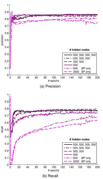
4.11 Precision and recall scores . . . 93

4.12 F-measure scores . . . 94

5.1 Diagram of an LRF-RBM . . . 104

5.2 Diagram of a hidden node receptive field mask . . . 106

5.3 Diagram of LRF-DBN and LRF-DNN training . . . 113

6.1 LRF-RBM training on face images . . . 125

6.2 Examples of RBM features . . . 126

6.3 Examples of non-face-specific LRF-RBM features . . . 127

(11)

6.4 Example features learnt by an RBM on the second layer of an

LRF-DBN . . . 128

6.5 LRF-RBM receptive field maps learnt on MNIST . . . 128

6.6 LRF-DBN receptive field and centre maps . . . 129

6.7 Comparison of the LRF-DBN and DBN feature hierarchies . . . . 130

6.8 SREs on the left, right, top, and bottom face completion tasks . . 133

6.9 SREs on the eyes, mouth, and random area face completion tasks 134 6.10 Comparison of DBN and LRF-DBN infilling iterations . . . 135

6.11 Example left and right completions . . . 137

6.12 Example top and bottom completions . . . 138

6.13 Example eye and mouth area completions . . . 139

6.14 Example random area completions . . . 140

6.15 Comparison of LRF-RBM and RBM SRE scores on a reconstruc-tion task . . . 141

6.16 Comparison of LRF-DNN and DNN autoencoder SRE scores . . . 142

6.17 Comparison of LRF-DNNs trained with different pretraining meth-ods . . . 145

6.18 Comparison of different LRF-DNN parameter choices . . . 146

6.19 Example RBM and LRF-RBM test image reconstructions . . . 147

6.20 Example DNN and LRF-DNN test image reconstructions calcu-lated from 500-length codes . . . 148

6.21 Example DNN and LRF-DNN test image reconstructions calcu-lated from 100-length codes . . . 149

A.1 Example frames from the complete set of training and test videos 167 A.2 Example positive and negative class test images . . . 168

B.1 Examples of non-face-specific LRF-RBM features learnt on LFW . 170 B.2 Visualisation of the LRF-DBN and DBN feature hierarchies . . . 176

(12)

List of Tables

6.1 SREs of DBNs and LRF-DBNs on the left, right, top, bottom, eyes, mouth, and random area completion tasks . . . 132 6.2 SREs of DNN and LRF-DNN reconstructions obtained from

500-length codes . . . 143 6.3 SREs of DNN and LRF-DNN reconstructions obtained from

100-length codes . . . 144

(13)

Abbreviations

CD contrastive divergence learning

CD1 single-step contrastive divergence learning

CDn n-step contrastive divergence learning

ConvNet convolutional neural network

DAG directed acyclic graph

DBN deep belief network

DNN deep neural network

DoG difference-of-Gaussians

EM expectation-maximisation

FFA fusiform face area

GPU graphics processing unit

IBP Indian buffet process

LFW Labeled Faces in the Wild

LGN lateral geniculate nucleus

LN linear-nonlinear model

LRF-DBN local receptive field constrained deep belief network LRF-DNN local receptive field constrained deep neural network

LRF-RBM local receptive field constrained restricted Boltzmann machine xii

(14)

Nomenclature xiii

OFA occipital face area

OMS object motion sensing

PCA principal component analysis

RBM restricted Boltzmann machine

SD standard deviation

SPI simulated photoreceptor input

SRE squared reconstruction error

SVM support vector machine

Notation

< . >φ expectation under the distribution φ

.(L) architecture of hidden layer trained by an LRF-RBM

a visible node biases in an RBM

b hidden node biases in an RBM

C recall

E(v,h) energy given visible and hidden node states

learning rate

F F-measure score

f n number of false negatives

f p number of false positives

G(σRF_{, k}₎ _{Gaussian filter with SD}_σRF _{and filter size}_k

h hidden node states in an RBM

H hidden layer in an RBM

H(., .) cross-entropy error

Hi ith hidden layer in a DBN or DNN

Ii _{weight image of hidden node} _h

(15)

k filter size used during LRF-RBM training

k filter sizes used for training consecutive layers of an LRF-DBN

n number of visible nodes in an RBM

N element-wise transformation used during LRF-RBM training

m number of hidden nodes in an RBM

p ground-truth label

ˆ

p predicted probability of classes

P precision

p(.) probability

R receptive field masks in an LRF-RBM

σ SDs of Gaussian visible nodes in an RBM

σRF _{SD of Gaussian receptive field constraints in an LRF-RBM}

σRF SDs of Gaussian receptive field constraints on consecutive layers of an LRF-DBN

tn number of true negatives

tp number of true positives

v visible node states in an RBM

V visible layer in an RBM or DBN

(16)

1

Introduction

In this chapter, I provide the background and motivation behind the research described in this thesis, introduce the approach taken, and summarise the main goals and contributions of the presented work.

1.1

Motivation

Research described in this thesis is motivated by the importance of understanding more about neural processing of visual information, the challenge of improving the performance of algorithms for high-level interpretation of visual data, and the widespread potential advantages of developing better computational models of information processing units within the visual pathway.

1.1.1 Computational Vision Systems

The design of computational methods for automatically interpreting visual data holds huge commercial and academic value but remains a highly challenging task. Advancements in this area can generate great impact within technology, security, and medicine with potential applications ranging from face recognition, intelli-gent image search engines and advanced modes of human-computer interaction to the design of navigation aids and devices for visually impaired people.

(17)

Fuelled by such interest, within the field of machine learning and computer vision much research has focused on the development of learning algorithms for understanding high-level semantics in visual data. Even with recent advance-ments, artificial vision systems still lag behind the highly efficient and accurate human visual system. Therefore, it is highly plausible that gaining more insight into how visual recognition is implemented within the brain can be the key to lift the performance of computational vision systems to a greater level.

1.1.2 Biological Visual Information Processing

The highly accurate vision of humans and other biological systems has long been within the centre of interest in neuroscience and biology. This great effort has brought about important discoveries regarding the morphology and functionality of neural cells and networks. However, our knowledge of visual information processing circuits and the specific roles of cells within the visual pathway is still far from complete.

Although numerous experiments have been conducted on different parts of the visual pathway, due to the high number, diverse functionality and complex con-nection patterns of neurons, understanding mechanisms behind biological visual processing remains a challenging open problem. Even well studied processing units, such as retinal neural networks contain a number of mysterious cell types whose functionality is yet unrevealed (Masland, 2012).

1.1.3 Computational Modelling of Biological Vision

Extending our knowledge regarding neural processing of visual information is not only important for neuroscientific and medical research but is a key challenge, underpinning many areas of machine learning, cognitive science, and intelligent

(18)

Chapter 1 Introduction 3

systems research.

Designing computational models of circuits within the visual pathway can greatly improve our understanding of biological visual information processing and can, hence, provide a more informed background for the design of visual data processing units, such as retinal implants. Furthermore, modelling mechanisms of biological vision can yield important practical benefits for algorithm design in machine learning, image processing, and computer vision.

A key motivation behind the modelling of biological vision is, therefore, to answer questions about the way biological systems process visual information and transfer this knowledge into the production of artificial vision systems, such as machine learning and computer vision algorithms or retinal implant designs.

1.2

The Proposed Approach

Modelling studies have traditionally focused on directly implementing function-alities of visual information processing cells and circuits based on our current knowledge, obtained from biological studies, regarding the workings of the vi-sual system. Nowadays however, with the constant advancement in experimental equipment and methodology, this ‘current knowledge’ changes ever so rapidly. Due to incomplete understanding of visual processing mechanisms in biological systems, designing robust computational models of these processes prompts one to account for uncertainty and unknown details.

Consequently, this thesis proposes a flexible data-driven approach that offers great potential for modelling in this uncertain environment. To model visual information processing mechanisms, I investigate existing deep learning methods and probabilistic models, e.g. deep belief networks (DBNs) (Hinton et al., 2006), and propose novel deep learning algorithms.

(19)

Deep learning methods, such as DBNs, deep neural networks (DNNs), and convolutional neural networks (ConvNets) (LeCun et al., 1998), extract multiple layers of feature detectors from data, where the consecutive layers correspond to increasingly abstract representations of information. DBNs can be trained efficiently by utilising a layer-wise unsupervised pretraining phase using restricted Boltzmann machines (RBMs) (Smolensky, 1986) on each consecutive layer, which can be followed by a supervised fine-tuning with backpropagation resulting in a DNN (Hinton et al., 2006). Deep learning methods have gained outstanding popularity in recent years owing to their state-of-the-art results achieved on a number of challenging machine learning and computer vision benchmarks.

The retina and the visual cortex exhibit an inherently multi-layered structure which lends itself naturally to modelling with deep learning models. The first part of this thesis investigates deep networks for modelling the earliest stages of the visual pathway, such as mechanisms implemented by the retina. Subsequently, novel deep learning methods are proposed for solving complex visual tasks, which require higher-level understanding of visual information. An example of such a task investigated here is face completion, which involves the occipital face area

(OFA) and thefusiform face area (FFA) of the visual cortex (Chen et al., 2010).

1.2.1 Early Visual Processing

Modelling biological information processing within early stages of the visual path-way, such as the retina, the thalamic lateral geniculate nucleus (LGN), and visual area V1, has key potential for advancing the field of retinal implant engineering and improving image processing and computer vision algorithms.

As opposed to strict traditional methods, I advocate a data-driven approach for modelling the retina and early visual processing. Instead of making

(20)

assump-Chapter 1 Introduction 5

tions regarding the morphology of retinal circuits, I strive to construct models which can automatically learn functional properties of the retinal network. To this end, I train deep learning models, DBNs and DNNs, on my specially devised dataset which simulates input reaching a small area of the retina.

Although DBNs have been used for modelling functionality of certain V1 and V2 cells (Lee et al., 2008), so far, less attention has been given to utilising the great potential of DBNs for modelling lower-level mechanisms, such as retinal processes, in detail.

Here, I address this issue by showing the proposed models are capable of discovering retinal functionality by learning from simulated retinal photoreceptor input data in an unsupervised setting. Among other features of early visual processing, the networks learn feature detectors similar to retinal ganglion cells. Additionally, classification performance is measured on a circular spot detection task, which approximates an early visual processing functionality, and results confirm the advantage of multi-layered network models.

The experiments, thereby, demonstrate that DBNs and DNNs have great potential for modelling feature detection implemented by the retina. Algorithms that can learn to replicate retinal functionality may provide important benefits for retinal prosthesis design. Such methods can increase the fidelity of visual information processing in a prosthetic device to real retinal functions, resulting in better vision restoration.

The photoreceptor input dataset and the analysis of experiments with DBN-and DNN-based retinal models trained on these data were previously described by Turcsany et al. (2014).

(21)

1.2.2 High-Level Visual Information Processing

In this thesis, I introduce novel deep learning methods, and using challenging visual tasks inspired by cortical functions, I demonstrate the methods’ great capability for modelling high-level visual information processing.

Despite successful attempts in applying deep learning methods to model vi-sual cortical areas (Lee et al., 2008), primary emphasis in the literature has been given to improving the performance of deep learning on visual recognition tasks, rather than increasing the fidelity of deep architectures to neural circuits of the visual pathway. Consequently, a main goal of the research presented here is to introduce deep learning architectures which more closely resemble biological neural networks of the visual pathway, while retaining the models’ flexibility and great performance on visual recognition tasks.

To address this, I investigate the introduction of biologically inspired struc-tural constraints into deep learning architectures and training methods, and show how such architectural changes can improve RBM, DBN, and DNN models. Also, I propose a novel RBM training method which improves the capability of the model to adapt its structure according to particularities of the input data. Util-ising this method during deep network training results in models with increased flexibility.

1.2.3 Novel Methods

This thesis proposes a novel unsupervised RBM-based model, the local recep-tive field constrained RBM (LRF-RBM), which imposes Gaussian constraints on feature detector receptive fields, thereby limiting the spatial scope of detectors. Concurrently with learning the appearance of features, LRF-RBMs can discover an advantageous non-uniform placement of feature detectors automatically from

(22)

data. This way, the LRF-RBM training encourages the emergence of local fea-ture detectors and, at the same time, improves feafea-ture detector coverage over key areas of the visual space.

Furthermore, this thesis introduces novel biologically inspired deep network architectures, the local receptive field constrained DBN and DNN (LRF-DBN and LRF-DNN). Training of both models starts by an unsupervised phase using LRF-RBMs with increasing receptive field sizes to learn consecutive layers. For LRF-DNNs, fine-tuning of the network weights follows, which in the experiments presented here comprises of training autoencoder networks with backpropagation on an image reconstruction task.

On the challenging ‘Labeled Faces in the Wild’ (LFW) face dataset, I show how LRF-RBM feature detectors automatically converge to important areas within face images, e.g., eyes and mouth, forming feature hubs. Also, a com-parison of generative models confirm that LRF-DBNs, trained layer-wise with LRF-RBMs, perform face completion tasks better than DBNs. Moreover, unlike DBNs, LRF-DBNs learn a feature hierarchy which exhibits part-based compo-sitionality. On the same dataset, dimensionality reduction experiments demon-strate the superiority of LRF-DNN autoencoders compared to DNNs for recon-structing previously unseen face images with a limited number of nodes. In addi-tion to obtaining lower reconstrucaddi-tion errors, LRF-DNN reconstrucaddi-tions better retain fine details of faces, such as mouth and nose shapes, directions of gaze, and facial expressions.

LRF-RBM, LRF-DBN, and LRF-DNN models, together with the analysis of the conducted experiments, were introduced by Turcsany and Bargiela (2014) and Turcsany et al. (2016).

(23)

1.3

Goals and Contributions

Work in this thesis was set out to show important benefits of forging a stronger connection between deep learning and the computational modelling of biological vision. Advantages, I argue, are twofold: on the one hand, flexible deep learning methods can reduce the need for handcrafted circuits by learning powerful models of visual information processing units automatically from data. On the other hand, improving the similarity of deep learning models to neural networks of the visual pathway can boost the performance of deep learning on challenging visual tasks.

The key contributions of this thesis are as follows:

(i) deep learning (DBN and DNN) models of the retina and early vision, which comply with a novel data-driven approach to retinal modelling;

(ii) a new simulated photoreceptor input dataset and a classification task ap-proximating early visual processing functionalities;

(iii) experiments demonstrating the great generative, reconstruction, and clas-sification capabilities of the proposed retinal models;

(iv) experiments confirming the models’ capability to learn feature detectors similar to difference-of-Gaussians and Gabor filters, common models of retinal ganglion, LGN, and V1 simple cells, and thereby demonstrating the suitability of DBNs and DNNs for modelling functions of the retina and early vision;

(v) development of a novel local receptive field constrained RBM (LRF-RBM), which uses biologically inspired receptive field constraints to encourage the

(24)

emergence of local features;

(vi) an adaptation of contrastive divergence learning (Hinton, 2002) which in-cludes receptive field constraints and

(vii) a mechanism which, concurrently with the learning of LRF-RBM features, can discover advantageous non-uniform feature detector placements from data by automatically identifying important locations within the visual space;

(viii) the development of LRF-DBN and LRF-DNN deep learning models, where LRF-RBMs are utilised during training to obtain architectures inspired by visual cortical organisation;

(ix) experiments on the ‘Labeled Faces in the Wild’ face image dataset demon-strating LRF-DBNs can learn a feature hierarchy which exhibits part-based composition;

(x) experiments showing LRF-DBN generative models perform face completion superior to DBNs and

(xi) LRF-DNN autoencoders obtain better dimensionality reduction results than DNNs, thereby demonstrating LRF-DBNs and LRF-DNNs can extract highly compact representations of visual information and can constitute powerful models of high-level visual information processing.

This thesis presents some novel methods and experimental results which were first described by Turcsany and Bargiela (2014) and Turcsany et al. (2014, 2016).

(25)

1.4

Overview

This thesis is organised as follows. Chapter 2 introduces the concept of deep learning and training algorithms for deep networks. Chapter 3 presents my ap-proach to retinal modelling and describes findings and open questions regarding the workings of the retina. My proposed models of the retina and early vision are evaluated in Chapter 4. Chapter 5 introduces my novel deep learning archi-tectures and training algorithms. Experiments evaluating these novel methods and proposed models of high-level visual information processing are presented in Chapter 6. Chapter 7 summarises the findings of this work and concludes the thesis. Finally, possible avenues for future work are suggested in Chapter 8.

(26)

2

Deep Learning

This chapter introduces the concept of deep leaning and describes the learning algorithms behind some established deep learning methods, which will be referred to in Chapters 4 and 5.

2.1

The Deep Learning Shift

Deep learning has emerged as a highly popular direction within machine learning research with the aim of developing methods which can extract multiple layers of features automatically from data. Deep learning algorithms create multi-layer representations of patterns present in the data, where each consecutive layer ex-ecutes the detection of increasingly complex features. Higher-level feature detec-tors are constructed using features from lower layers; hence, this representation scheme exhibits increased abstraction levels on each consecutive layer.

A strong analogy with biological neural information processing can be no-ticed, as it is widely accepted that brains of humans and other biological entities also utilise multi-level representation schemes for the efficient extraction of in-formation from sensory input (Coogan and Burkhalter, 1993; Felleman and Van Essen, 1991; Hinton, 2007; Konen and Kastner, 2008; Van Essen and Maunsell, 1983; Wessinger et al., 2001). Such an organisation with multiple consecutive

(27)

(a)

. . .

(b)

Figure 2.1 (a) Layers I-VI of the visual cortex are shown in a cross-section, illustrating the hierarchical organisation of the visual cortex. Increasing numbers correspond to higher-level processing areas. Original image source: Schmolesky (2000). (b) The concept of deep learning, whereby consecutive layers of representation correspond to features of increasing complexity, is illustrated in the context of visual processing. Lower layers detect simple features, such as edges and shapes, while higher layers correspond to complex features, such as faces and objects.

processing layers can be observed in, for example, the retina and the cortex. Figure 2.1(a) demonstrates the multi-layer structure of the visual cortex in a cross-section, while Figure 3.1(a)–(b) show the numerous processing layers of the retina. Figure 2.1(b) illustrates the concept of deep learning and the simi-larity between cortical processing and deep learning.

A highly advantageous property of deep learning algorithms is their ability to learn features automatically from data, which eliminates the need for hand-crafted feature detectors. These flexible models have been shown to outperform traditional approaches on numerous information processing tasks, leading to their application not only in academic research but in a variety of industrial sectors. The explored application domains range from computer vision (see Section 2.1.1),

(28)

Chapter 2 Deep Learning 13

speech recognition (Collobert and Weston, 2008; Graves et al., 2013), text anal-ysis (Salakhutdinov and Hinton, 2009b), reinforcement learning in games (Mnih et al., 2013, 2015), robot navigation (Giusti et al., 2016), and time-series predic-tion (Kuremoto et al., 2014; Prasad and Prasad, 2014) to even art (Gatys et al., 2015; Mordvintsev et al., 2015). An area where deep learning has had a highly remarkable influence is the visual information processing field.

2.1.1 Impact in Computer Vision

Many areas of visual information processing research, such as computer vision, have traditionally relied on the handcrafted SIFT (Lowe, 2004), SURF (Bay et al., 2008) or similar local feature detectors (Li et al., 2014c; Rublee et al., 2011), often followed by bag-of-words type quantisation techniques (Sivic and Zisserman, 2003; Tao et al., 2014; Turcsany et al., 2013), for the successful design of accurate systems (e.g. Battiato et al., 2007; Lin and Lin, 2009; Zhang et al., 2015).

With the emergence of deep learning, however, focus has shifted towards au-tomatically learning a hierarchy of relevant features directly from input data instead of applying generic, handcrafted feature detectors. Such feature hierar-chies can be well captured by multi-layer network models, such as DBNs, DNNs or ConvNets. When applied to visual recognition, multi-level representations are especially suitable for modelling complex relationships of visual features, and the hierarchical structure allows one to represent principles such as composition and part-sharing in an intuitive way. Consequently, deep architectures possess great potential for solving visual tasks, and in recent years such methods have demon-strated exceptional improvements over the existing state of the art, reaching and in some cases surpassing human-level performance (e.g. Cireşan et al., 2012;

(29)

Giusti et al., 2016; He et al., 2015b; Mnih et al., 2015; Sun et al., 2015). Deep learning methods routinely achieve state-of-the-art results on computer vision benchmarks, including datasets for handwritten digit recognition (Cireşan et al., 2012, 2011b), object recognition and classification (Cireşan et al., 2011b; He et al., 2015a,b; Krizhevsky et al., 2012; Simonyan and Zisserman, 2015; Szegedy et al., 2014), face verification (Ding and Tao, 2015; Schroff et al., 2015; Sun et al., 2014), and human pose estimation (Charles et al., 2016; Pfister et al., 2015; Tompson et al., 2014; Toshev and Szegedy, 2014).

2.1.2 Deep Network Models

Deep neural networks and deep learning models have been investigated since the late 1960s (see, e.g., Ivakhnenko, 1971; Ivakhnenko and Lapa, 1965); however, for a number of years, interest in such models has largely been overshadowed by the success of ‘shallow’ models, such as support vector machines (SVMs) (Cortes and Vapnik, 1995; Vapnik, 1995).

A recent, remarkable surge in the popularity of deep learning has been trig-gered by the work of Hinton et al. (2006), where a highly efficient DBN model and training algorithm was introduced. This has been followed by the applications of the method for image classification, dimensionality reduction, and for document clustering and retrieval (Hinton and Salakhutdinov, 2006a; Salakhutdinov and Hinton, 2009b).

To learn a multi-layer generative model of the data where each higher layer corresponds to a more abstract representation of information, Hinton et al. (2006) train a DBN first layer by layer using RBMs. The network parameters learnt during this unsupervised pretraining phase are subsequently fine-tuned in a su-pervised manner with backpropagation (Linnainmaa, 1970, 1976; Werbos, 1982),

(30)

resulting in a DNN. Such models were shown to be superior to principal com-ponent analysis (PCA) for dimensionality reduction (Hinton and Salakhutdinov, 2006a).

Since the introduction of this efficient training method for deep networks, deep learning research has gained increased interest, resulting in a wide-ranging academic and commercial adoption of deep learning techniques. A number of successful applications of DBNs, DNNs, and other deep architectures, for exam-ple convolutional DBNs (Lee et al., 2009a), ConvNets (LeCun et al., 1998), deep recurrent neural networks (Fernández et al., 2007; Graves et al., 2013), sum-product networks (Poon and Domingos, 2011), and deep Boltzmann machines (Salakhutdinov and Hinton, 2009a), have been presented. Within computer vi-sion, the potential of these and similar methods for automatically learning mean-ingful features from input data and thereby providing improved models has been demonstrated on:

(i) object recognition (He et al., 2015a,b; Kavukcuoglu et al., 2010; Krizhevsky et al., 2012; Le et al., 2012; Nair and Hinton, 2010; Rozantsev et al., 2015; Simonyan and Zisserman, 2015; Szegedy et al., 2014; Xia et al., 2015), (ii) image classification (Cireşan et al., 2011a, 2012, 2011b; Giusti et al., 2016;

Hinton and Salakhutdinov, 2006a; Jaderberg et al., 2015; Larochelle et al., 2007; Ranzato et al., 2006; Salakhutdinov and Hinton, 2007),

(iii) face image analysis (Ding and Tao, 2015; Huang et al., 2012; Nair and Hinton, 2010; Ranzato et al., 2011; Schroff et al., 2015; Sun et al., 2015, 2014; Turcsany and Bargiela, 2014; Turcsany et al., 2016; Zhu et al., 2013), (iv) human pose estimation (Charles et al., 2016; Pfister et al., 2015, 2014;

(31)

(v) further visual tasks (Dosovitskiy et al., 2015; Eslami et al., 2012; Gatys et al., 2015; Mnih et al., 2013, 2015; Su et al., 2015; Turcsany et al., 2014). Besides the analysis of visual data, deep learning methods have been used with great success on problems concerning the analysis of

(i) text (Hinton and Salakhutdinov, 2006a; Salakhutdinov and Hinton, 2009b), (ii) speech (Amodei et al., 2015; Collobert and Weston, 2008; Fernández et al.,

2007; Graves et al., 2013; Lee et al., 2009b),

(iii) further types of audio data (Lee et al., 2009b; Maniak et al., 2015), and (iv) time-series data (Kuremoto et al., 2014; Prasad and Prasad, 2014).

Through distributed implementations (Le et al., 2012) or with the application of graphics processing units (GPUs) (Cireşan et al., 2011a; Krizhevsky et al., 2012), deep learning methods have been shown to scale up and provide excellent performance even on large-scale problems.

2.2

Multi-layer Representations in the Brain

As mentioned in Section 2.1, the concept of deep learning shows similarity to neural processing, since brains also represent information extracted from sensory input on multiple abstraction levels (see Figure 2.1). Furthermore, deep network models display structural resemblance to biological visual information processing units. For example, as Chapter 3 will demonstrate, the structure of mammalian retinae is inherently multi-layered: the different cell types (i.e. rods, cones, hor-izontal cells, bipolar cells, amacrine cells, and ganglion cells) are organised into multiple consecutive processing layers such as the photoreceptor, outer plexiform, and inner plexiform layers, which implement increasingly complex functions. On

(32)

a larger scale, visual information processing is executed by consecutive areas of the visual pathway (i.e. retina, LGN, V1, V2, etc.) through the extraction of more and more abstract representations of patterns.

Due to the structural analogy, it is not surprising deep learning methods have been used successfully to model certain neural information processing units. For example, Lee et al. (2008) have shown the suitability of DBNs for modelling feature detection in the V1 and V2 areas of the visual cortex. While their study did not focus on the exact replication of neural connectivity patterns in visual cortical areas, features automatically learnt by the network show similarity to typical V1 and V2 feature detectors. These results indicate that such models can successfully learn functionalities implemented by neural networks of the visual pathway and can therefore be applied to model biological visual information processing on a more abstract level.

Despite this achievement in neural modelling, primary emphasis in prior works has been assigned to improving the performance of deep learning on vi-sual recognition tasks, rather than increasing the fidelity of deep architectures to real neural circuits of the visual pathway. A key contribution of my work has been to take a step towards filling this gap by proposing deep network structures that more closely resemble biological neural networks of the visual pathway. The proposed models not only retain the characteristic flexibility of deep networks but further increase their performance on visual recognition tasks. Such archi-tectures possess high potential for learning improved computational models of visual information processing in the retina and the visual cortex.

Chapter 4 introduces my DBN-based retinal model, which provides a further proof for the suitability of deep learning methods for modelling neural informa-tion processing units. This model has been shown to successfully learn ganglion

(33)

cell functionality from simulated photoreceptor input data and execute an early vision task (Turcsany et al., 2014).

Chapter 5 describes my LRF-DBN and LRF-DNN models (Turcsany and Bargiela, 2014; Turcsany et al., 2016), which have been designed with the aim to increase the structural similarity of deep network models to neural networks of the visual pathway. Chapter 6 demonstrates that this novel deep learning model can successfully implement face completion tasks, known to be executed in high-level processing areas of the human visual cortex (Chen et al., 2010).

Chapters 4 to 6 build on certain concepts of DBN training, which will be in-troduced in the following sections. These sections describe the steps of RBM and DBN training and introduce common DBN-based models, such as autoencoders.

2.3

Restricted Boltzmann Machines

The first, unsupervised phase of Hinton et al.’s (2006) DBN training utilises RBMs for learning each layer of the representation.

RBMs (Smolensky, 1986) are probabilistic graphical models which originate from Boltzmann machines (Hinton and Sejnowski, 1983). The energy-based Boltzmann machine model contains visible nodes, whose states are observed, and unobserved hidden nodes and has no constraints on which types of nodes can be connected.

RBMs, on the other hand, do not contain links between nodes of the same type, hence the ‘restriction’ (see Figure 2.2 for an illustration). RBMs are there-fore bi-partite graphs, consisting of a visible and a hidden layer, where symmet-ric connections exist between layers but not within layers. As a result, they are significantly quicker to train than Boltzmann machines due to the conditional independence of hidden nodes given visible nodes and vice versa.

(34)

This efficiency in training has resulted in widespread use of RBMs and their variants within machine learning, including applications to:

(i) document retrieval (Hinton and Salakhutdinov, 2006a; Xie et al., 2015), (ii) collaborative filtering (Georgiev and Nakov, 2013; Salakhutdinov et al.,

2007),

(iii) link prediction (Bartusiak et al., 2016; Li et al., 2014a,b; Liu et al., 2013), (iv) multi-objective optimisation problems (Shim et al., 2013),

(v) visual tasks (Elfwing et al., 2015; Eslami et al., 2012; Hinton and Salakhut-dinov, 2006a; Kae et al., 2013; Memisevic and Hinton, 2007; Nair and Hin-ton, 2010; Nie et al., 2015; Ranzato et al., 2011; Salakhutdinov and HinHin-ton, 2009a; Sutskever et al., 2008; Turcsany and Bargiela, 2014; Turcsany et al., 2014, 2016; Wu et al., 2013; Xu et al., 2015; Zhao et al., 2016),

(vi) modelling of motion capture data (Mittelman et al., 2014; Sutskever et al., 2008; Taylor and Hinton, 2009; Taylor et al., 2006) as well as

(vii) speech and audio data analysis (Dahl et al., 2010; Lee et al., 2009b; Maniak et al., 2015).

In visual recognition tasks visible nodes usually correspond to visual input coordinates (e.g. image pixels), while hidden nodes represent image feature de-tectors and can, thus, be seen as models of neurons in the visual pathway.

The following sections will first discuss how RBMs with binary visible and hidden nodes are trained, then show how Gaussian visible nodes can be used to model real-valued data. For more details regarding the training of RBMs, refer to (Hinton, 2002, 2012; Hinton et al., 2006; Nair and Hinton, 2010).

(35)

H

V

Figure 2.2 Diagram showing a restricted Boltzmann machine. The model consists of a visible (V) and a hidden layer (H), where connections only exist between layers but not within layers. V corresponds to the input data coordinates, while hidden nodes in

H are used for learning features from the input data.

2.3.1 The RBM Model

The probability that an RBM model assigns to a configuration (v,h) of visible and hidden nodes can be calculated using the energy function (Hopfield, 1982) of the model. In the case of binary visible and hidden nodes, the RBM’s energy function takes the form:

E(v,h) =−aTv−bTh−vTWh, (2.1)

where v ∈ {0,1}n _and _h _{∈ {}₀_,₁_}m _{describe the binary states of the visible}

and the hidden nodes, respectively, W ∈ _Rn×m _{is the weight matrix defining}

the symmetric connections between visible and hidden nodes, whilea ∈_Rn _and

b∈_Rm _{provide the biases of visible and hidden nodes, respectively.}

The probability of a joint configuration (v,h) is then given by:

p(v,h) = e

−E(v,h)

P

η,µe−E(η,µ)

. (2.2)

(36)

be obtained after marginalising out h:

p(v) = P he−E(v,h) P η,µe−E(η,µ) . (2.3)

Unsupervised learning in an RBM aims at increasing the log probability of the training data, which is equivalent to reducing the energy of the training data. During the training phase, the probability of a given training example can be increased (the energy reduced) by altering the weights and biases. The following learning rule can be applied to maximise the log probability of the training data by stochastic steepest ascent:

∆wij =(< vihj >data −< vihj >model), (2.4)

where is the learning rate and < . >φ is used for denoting expectations under

the distribution φ.

Due to the conditional independence properties in RBMs, sampling for vihj

according to the distribution given by the data is simple. In the case of an RBM with binary visible and hidden nodes, the probability of a hidden nodehj turning

on given a randomly chosen training examplev is:

p(hj = 1|v) =

1

1 +exp(−bj−Piviwij)

; (2.5)

that is the logistic sigmoid function applied to the total input of the hidden node. An example of an unbiased sample is then given byvihj. Sampling for the visible

(37)

states h of the hidden nodes is:

p(vi = 1|h) =

1

1 +exp(−ai−Pjhjwij)

. (2.6)

On the other hand, calculating an unbiased sample of < vihj >model would

require a long sequence of alternating Gibbs sampling between the visible and hidden layers; therefore, in practice approximations are normally applied.

2.3.2 Contrastive Divergence Learning

Contrastive divergence learning (CD) (Hinton, 2002) is an efficient approximate training method for RBMs. Even though CD only broadly approximates the gradient of the log probability of the training data (Hinton, 2002, 2012), in practice CD has been found to produce good models. RBMs trained efficiently using CD and also ‘stacked’ RBMs, used for pretraining a DBN, are powerful tools for learning generative models of visual, text, and further types of complex data.

In the single-step version (CD1) of contrastive divergence learning, each

train-ing step corresponds to one step of alternattrain-ing Gibbs sampltrain-ing between the visible and hidden layers starting from a training example. The algorithm proceeds as follows:

(i) first, the visible states are initialised to a training example;

(ii) then, binary hidden states can be sampled in parallel1 according to Equa-tion (2.5);

(iii) followed by the reconstruction phase, where visible states are sampled using Equation (2.6);

(38)

(iv) finally, the weights are updated according to:

∆wij =(< vihj >data −< vihj >reconst), (2.7)

whereis the learning rate, the correlation between the activations of visi-ble nodeviand hidden nodehj measured after (ii) gives< vihj >data, while

the correlation after the reconstruction phase (iii) provides< vihj >reconst2.

In order to obtain an improved model, the sampling stage in each step can be continued for multiple iterations, resulting in the general form of the CD algorithm: CDn, where n denotes the number of alternating Gibbs sampling

iterations used in a training step.

2.3.3 RBMs with Gaussian Visible Nodes

While RBMs with binary visible nodes are generally easier to train than RBMs with Gaussian visible nodes, the latter can learn better models of real-valued data, such as the simulated photoreceptor input data in Chapter 4 or the face images studied in Chapter 6.

In the case of Gaussian visible nodes the energy function changes to:

E(v,h) = X i (vi−ai)2 2σ2 i −X j bjhj − X i,j vi σi hjwij , (2.8)

where σi is the standard deviation corresponding to visible node vi. The

proba-bility of hidden node activation becomes:

p(hj = 1|v) =

1

1 +exp(−bj−Pi(vi/σi)wij)

, (2.9)

(39)

and the expected value of a Gaussian visible node (i.e. the reconstructed value) is given by: < vi >reconst=ai+σi X j hjwij . (2.10)

When Gaussian visible nodes are used instead of binary visible nodes, certain learning parameters may need to be adjusted (e.g. the learning rate generally has to be lowered).

2.4

Deep Belief Networks

Deep belief networks are probabilistic graphical models capable of learning a gen-erative model of the input data in the form of a multi-layer network. Within these models, multiple consecutive layers facilitate the extraction of highly non-linear features, making DBNs capable of learning powerful models of even complex data distributions. It has been shown DBNs, given certain architectural constraints, are universal approximators (Sutskever and Hinton, 2008). Furthermore, the trained models define a generative process, which enables the construction of new datapoints that fit the modelled input data distribution. Such a generative DBN is illustrated in Figure 2.3.

Deep belief networks can be trained efficiently according to the method of Hinton et al. (2006) by first pretraining the network in a ‘greedy’ layer-by-layer fashion with unsupervised RBMs in order to learn a favourable initialisation of the network weights. In this process, after using an RBM to train a hidden layer, the weights become fixed, and the activations on this hidden layer provide the input to the next RBM.

Once pretraining has been completed, the multi-layer network can be fine-tuned either as a generative model or discriminatively, to solve a specific task.

(40)

Figure 2.3 Diagram of a DBN with 4 hidden layers trained on an image dataset.

V denotes the visible and H1–H4 the hidden layers. The blue arrows correspond to the generative model, while the upward-pointing red arrows indicate the direction of recognition. In the generative model, the top two layers form an associative memory.

Fine-tuning can be conducted by, e.g., backpropagation or a variant of the ‘wake-sleep’ algorithm (Hinton, 2007; Hinton et al., 2006; Hinton and Salakhutdinov, 2006a).

In the following, common use cases and applications of DBN models are introduced.

2.4.1 Generative Model

Hinton et al.’s (2006) DBN generative model is composed of multiple consecutive layers, where the lower layers contain directed connections, while the top two layers have undirected connections and form an associative memory (Hopfield, 1982). If certain conditions are met, it can be shown that adding a further hidden layer to a DBN produces a better generative model of the data (Hinton et al., 2006). Fine-tuning of a DBN with the aim of obtaining an improved generative model can be conducted using the ‘wake-sleep’ algorithm (Hinton et al., 1995,

(41)

H₁ V H₂ H₃ Class labels H₄

Figure 2.4 Schematic of a DBN generative model containing 4 hidden layers (H1–H4) used for generating images together with their class labels. V denotes the visible and

H1–H4 the hidden layers. The blue arrows correspond to the generative model, while the upward-pointing red arrows indicate the direction of recognition. H3, extended with the class label nodes, and H4 form an associative memory.

2006) after the greedy layer-wise pretraining phase.

A DBN generative model can either be trained completely unsupervised or, alternatively, labels can be introduced. The model proposed by (Hinton, 2007; Hinton et al., 2006) learns to generate new data together with the appropriate class labels. To this end, the penultimate layer of a DBN is extended with nodes corresponding to class labels, and the top RBM learns to model the data jointly with the labels (see diagram in Figure 2.4). It is possible to generate new images from a given class by executing alternating Gibbs sampling between the top two layers while appropriately clamping the value of the class labels, then calculating top-down activations. The capability of such a DBN to learn a generative model of handwritten digits was demonstrated on the MNIST dataset (Hinton et al., 2006).

The trained model can also be used for classification. In this case, bottom-up (i.e. recognition) activations are calculated after feeding in an example; then,

(42)

Chapter 2 Deep Learning 27 H₁ V H₂ H₃ Output Layer

Figure 2.5 Schematic of a DNN used for classification. The network contains a visible layerV corresponding to the input, 3 hidden layers (H1–H3), and an output layer with nodes corresponding to the classes.

while the bottom-up activations on the penultimate layer are kept fixed, alternat-ing Gibbs samplalternat-ing is conducted between the top two layers, and the probability of each class label turning on is compared.

2.4.2 Deep Neural Networks and Classification

Using backpropagation, a pretrained DBN can be explicitly tuned to solve a classification task. After the network has been pretrained layer by layer as a generative model, an output layer is added, where the nodes correspond to class labels. Then, backpropagation is performed on the training set to minimise classification error, which can, for example, be measured using the cross-entropy error:

H(p,pˆ) = −X i

piln ˆpi, (2.11)

where, given a training example, the true label defines p, while ˆpi denotes the

probability of the example belonging to categoryiaccording to the prediction of the model.

(43)

When backpropagation is used for fine-tuning, the resulting model is a deep neural network (DNN)3_{. A schematic diagram of such a classifier DNN is shown}

in Figure 2.5. These discriminatively fine-tuned models generally provide better performance on classification tasks than the generative classifier described in Sec-tion 2.4.1 (see Hinton, 2007). Such DNN models have achieved excellent results on challenging datasets, including the MNIST handwritten digit classification problem (Hinton et al., 2006).

In the context of retinal modelling, Chapter 4 analyses the performance of DNNs on a discriminative circle detection task and confirms the importance of pretraining.

2.4.3 Autoencoders

Autoencoder DNNs are used for dimensionality reduction of input data. Their multi-layer network architecture consists of an encoder and a decoder part, where the encoder part is trained to generate reduced-dimensional codes for input dat-apoints. From such an encoding, the decoder part is capable of calculating a reconstruction which approximates the original input example. A diagram of an autoencoder is shown in Figure 2.6.

Autoencoder DNNs are pretrained as DBNs where the top layer has fewer hidden nodes than the input dimension. Representations obtained on this layer therefore provide a lower-dimensional encoding of the input. This pretraining constitutes an initialisation for the encoder part of the deep autoencoder, while to obtain the decoder part, the pretrained layers are ‘unrolled’ by transposing the weights on each layer. The weight initialisations obtained for the encoder and decoder layers provide a starting point for backpropagation, whereby the encoder

(44)

Chapter 2 Deep Learning 29 H₁ V H₂ H3 H₄ decoder encoder

Figure 2.6 Schematic of a deep autoencoder neural network used for dimensionality reduction. The network consists of an encoder part, which calculates reduced-length codes (H2) for input examples, and a decoder part that can obtain a reconstruction (H4) from such an encoding.

and decoder are fine-tuned as one multi-layer network. During optimisation, the squared reconstruction error (SRE) is minimised, which is defined as the squared distance between the original data and its reconstruction. Salakhutdinov and Hinton (2009b) apply such an autoencoder to produce compact binary codes for documents in a text retrieval task.

Chapter 5 introduces a new type of deep autoencoder network, the LRF-DNN autoencoder, and compares results with the traditional method on a face image reconstruction task. A schematic of deep autoencoder training on this face dataset is shown in Figure 5.3(b) of Chapter 5.

A more detailed description of autoencoder training is provided by Hinton and Salakhutdinov (2006a), where fine-tuning of DBNs as classifiers is also described.

(45)

2.5

Learning the Structure of Deep Networks

Structure learning can improve the flexibility of a modelling approach by iden-tifying the best structural parameters of a model automatically during training. In the case of DBNs, such parameters describe the network architecture, i.e. the number of layers and the number of nodes in each layer.

A variety of approaches have been proposed in the literature for learning the structure of belief networks or the architectural parameters of a neural network. However, due to scalability issues, the use of structure learning methods on com-plex real-world problems is currently limited. In the following, a few promising approaches to structure learning are introduced with a primary focus on Bayesian non-parametric methods.

For learning the structure of belief networks, heuristic procedures (Heckerman et al., 1995) and evolutionary algorithms (Pelikan et al., 2001) have been explored in the literature, along with a structure learning extension of the expectation-maximisation (EM) algorithm (Dempster et al., 1977), called model selection EM, introduced by Friedman (1997).

Efficient structure learning is considerably easier to implement in certain restricted types of models, such as mixtures-of-trees, for which Meila and Jordan (2001) proposed an EM-based algorithm. In a more general setting, a method based on Mercer kernels was introduced by Bach and Jordan (2002) for learning the structure of graphical models. For a specific class of neural networks, Angelov and Filev (2004) developed a method that can adapt the networks’ structure in an online manner, thereby providing improved flexibility.

A popular approach is the use of Bayesian non-parametric methods for infer-ring structure (Ghahramani, 2012), which provides a principled way of learning

(46)

the structural parameters of a probabilistic model from data.

2.5.1 Bayesian Non-parametrics

Bayesian non-parametric methods allow for the introduction of suitable prior probability distributions over structural components of a model. Using standard probabilistic inference methods, the model structure can be inferred together with the model parameters. Commonly used priors include the Chinese restau-rant process (Aldous, 1985; Pitman, 2002), applied in the infinite mixture model, and the Indian buffet process (Griffiths and Ghahramani, 2005, 2011) for the in-finite latent feature model.

In a mixture model, each example belongs to a category, whereas a latent feature model represents objects by their sets of features. Each object can possess multiple features, and in the infinite latent feature model, the total number of available features is infinite. Fitting this model can be formalised as a problem to learn a sparse binary matrix, where rows correspond to objects, columns correspond to features, and elements of the matrix describe whether the given object possesses the given feature.

In the infinite model, the number of objects (rows) is finite and the number of features (columns) is infinite. To regularise the effective number of features in the model, i.e. features that are actually possessed by the objects, a suitable prior distribution has to be used. The Indian buffet process (IBP) defines a distribu-tion on infinite sparse binary matrices (finite row, infinite column) and therefore provides a suitable prior. Using the IBP the expected number of features per object will follow a Poisson distribution.

As demonstrated by Adams et al. (2010), the cascading (stacked) IBP is suitable for learning the structure of a sparse DBN from data, including the

(47)

number of layers, number of nodes per layer, and the type of each node: either binary or continuous valued. In this work, a flexible 2-parameter version of the IBP is used and inference is conducted using sampling. An IBP prior is also utilised in the work of Feng and Darrell (2015), where the structure of a deep convolutional network is learnt from data.

Non-parametric approaches are highly promising for learning the structure of networks; however, for some distributions, variational inference methods are not available and inference using sampling can take an extensive amount of time on complex models, which limits current use.

2.5.2 Hyperparameter Learning

In the case of neural networks, practical application of the methods is not only complicated by the difficulty of identifying a suitable network structure, but suc-cessful training also often requires extensive tuning of certain hyperparameters, such as the learning rate and momentum. By calculating the gradients of cross-validation performance with respect to the hyperparameters, Maclaurin et al. (2015) propose a method for automatically optimising any type of hyperparame-ter (e.g. network architecture, learning rate, and the distribution used for weight initialisation) in neural networks trained using stochastic gradient descent with momentum.

2.6

Feature Visualisation

In order to gain a deeper understanding of the internal representations used by a DBN to encode input data or the process a classifier DNN follows to make pre-dictions, it would be highly beneficial to examine the feature detectors learnt on each layer of the network. In the following, I will describe how feature detectors

(48)

on each layer of a deep network can be visualised when the network has been trained on image data.

As the weights of nodes on the first hidden layer correspond to image lo-cations, a visualisation of these features can be obtained in a straightforward manner by displaying the hidden nodes’ weight vectors in the shape of the input image data.

Visualisation of features on consecutive layers in a DBN or DNN is compli-cated by the presence of non-linearities on higher layers. However, by applying an approximate method used in prior work (Erhan et al., 2009; Lee et al., 2008, 2009a), a useful visualisation can still be obtained. For each hidden node on a higher layer, a feature visualisation can be constructed by using the connection weights to calculate a linear combination of those features from the previous layer that exhibited the strongest connections to the given higher-layer node. This way, feature visualisations can be calculated in a layer-by-layer manner.

Chapters 4 and 6 will use the above described method to show features of DBNs and DNNs trained for modelling the retina and face images.

2.7

Summary

This chapter has introduced the concept of deep learning together with recent advances within this line of machine learning research. Key steps of DBN and DNN training have been provided, including a description of the RBM model and the contrastive divergence learning algorithm.

As discussed, in recent years deep learning algorithms have obtained state-of-the-art status on a large number of machine learning and computer vision benchmarks. It is, however, not surprising given the recency of deep learning developments that various theoretical and practical questions in this area have

(49)

not yet been answered. It is still unclear what architectures are the most powerful for learning multi-layer representations and what training methods guarantee the most reliable learning performance alongside efficient computation. This applies especially to problems where the type of data or the learning task differs from the conventional cases. From a practical point of view, application of deep networks to challenging ‘real-world’ problems is non-trivial and the process often involves extensive parameter tuning.

Such challenges and the potential great benefits make investigations concern-ing deep architectures and suitable trainconcern-ing algorithms highly important for the advancement of machine learning research and related applications.

(50)

3

Modelling the Retina

This chapter describes the motivation behind designing computational models of the retina, summarises key knowledge concerning retinal cells and circuits, introduces previous computational models, and contrasts these methods with my novel approach to retinal modelling. I will also give examples of open questions regarding the workings of the retina and provide arguments for the suitability of my retinal modelling approach for the study of these questions.

3.1

Motivation for Retinal Modelling

Extending our knowledge of information processing mechanisms within the retina could lead to major advances in the design of learning algorithms for artificial retinae. Such algorithms are much sought after, as building better computational models of the retina is crucial for advancing the field of retinal implant engineer-ing and can also be beneficial for improvengineer-ing image processengineer-ing and computer vision algorithms.

Despite insights into the anatomy, physiology, and morphology of neural structures, gained through experimental studies, understanding biological vision systems still remains an open problem due to the abundance, diversity, and com-plex interconnectivity of neural cells. Retinal cells and networks are not exempt

(51)

from this rule even though they are relatively well studied. For example, recent studies have revealed a lot more complexit