Self-tuning one-class support vector machines for data classification

(1)

Self-Tuning One-Class Support Vector Machines

for Data Classification

by

©Yiming Qian

A thesis submitted to the School of Graduate Studies

in partial fulfilment of the requirements for the degree of Master of Science

Department of Computer Science Memorial University of Newfoundland

Jun 2014

(2)

Abstract

Support Vector Machine (SVM) based classifiers are most popular models for data classification in machine learning. To obtain high classification accuracy, parameter tuning methods such as cross-validation are often applied, which is however time-consuming. To address this problem, a simple, efficient and parameter-free algorithm is presented in this thesis. The algorithm is especially useful when dealing with datasets in the presence of label noise. Grown out of one-class SVM, the presented algorithm enjoys several distinct features: First, its decision boundary is learned based on both positive and negative examples, whereas the original one-class SVM training is only based on positive examples; Second, the internal parameters are self-tuned, which makes the algorithm handy to use even for first-time users. Compared with the benchmark method LIBSVM, the presented algorithm achieves comparable accuracy, while consuming only a fraction of the processing time. Applications in computer vision are presented to demonstrate the effectiveness of the algorithm.

(3)

Acknowledgements

First, I feel extremely lucky to have had the opportunity to study with my advisor Prof. Minglun Gong. It has been a great pleasure for me to work with him on several projects, including this thesis. I would like to thank him for his guidance, inspiration and support during my graduate studies. Prof. Gong strengthened my love for computer vision and machine learning, and shared his research experience with me. I have learned a lot about research methodology from him, as well as basic principles of being a better researcher. I would also appreciate his financial support for my life at Memorial.

Second, I would like to thank Dr. Yung-Yu Chuang, Dr. Antonio Criminisi, Dr. Stan Sclaroff, Dr. Yaser A. Sheikh, Dr. Seth Teller, Dr. Xue Bai, Dr. Jue Wang, Dr. Yu-Wing Tai, Mr. Inchang Choi, and Mr. Eduardo S. L. Gastal for sharing their datasets or experiment results used in this thesis with us or online.

Third, I would like to thank School of Graduate Studies and Department of Com-puter Science. Thanks to all staffs who helped me in the two years. I am also grateful to my friends at St. John’s Shibai Yin, Hao Yuan, Rose Reid and Yunhai Wang -for making my master study enjoyable. Without them, life at Memorial would be a lot more boring.

Last, I would like to thank my family for their love and support, especially my parents Chunyong Cai and Ping Qian, and my wife Huihong Niu. This thesis is dedicated to them.

(4)

List of Tables

(8)

List of Figures

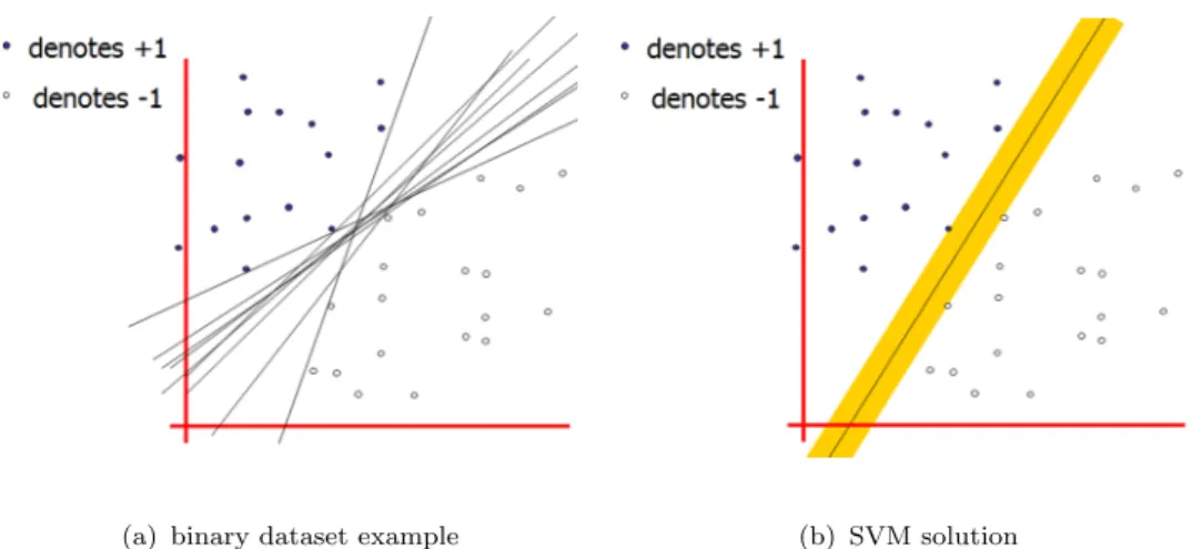
2.1 Given two classes of data points shown in (a), there are many possible linear classifiers. SVM training tries to find the one with the maximum margin (the one with the maximum width of the yellow part in (b)). . 11 2.2 After applying a nonlinear function ϕ, data points which is not

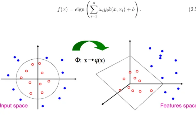
lin-early inseparable in their original input space can be split by a linear hyperplane in feature space. . . 12

3.1 Define an adjustable kernel k(u, v, σ) based on a normalized kernel

k(u, v). . . 24 3.2 Visualization of the classification results for the “threeclass” dataset.

Top row shows the selected support vectors with the corresponding σ

values illustrated using circles. Bottom row shows the decision maps, which encode the output scores from the three one-class SVMs using red, green, and blue channels respectively. Both black color in (a-b) and orange/cyan/magenta colors in (b-c) indicate regions with ambi-guities. . . 26

(9)

3.3 Visualization of the classification results when the dataset is corrupted with label noise, i.e., 5% of the random data have their labels changed. Under both fixed (a-d) and adaptive (e-h) Gaussian support situations, using adaptive cut-off values helps to limit the impacts of outliers. . . 28

4.1 Convergence of the conventional approach and the reweighting scheme. For a given set of examples (a), the decision map (b) obtained using the conventional approach under a very small decay rate is used as the ground truth. Comparing the decision maps generated after differ-ent iterations with the ground truth shows the convergence speeds of different approaches (c). . . 33 4.2 The effectiveness of self-tuningσ. Classification accuracy comparisons

between self-tuned σ (red) and one-class SVM (blue) trained under different σ values are plotted. . . 34 4.3 The effectiveness of self-tuningχ. Classification accuracy of self-tuned

χ(red), fixedχ= 0.1 (green), and fixedχ= 0.5 (blue) under increasing label noise is compared. . . 35 4.4 Comparison between STOCS and LIBSVM under Gaussian kernel.

Top left shows the classification accuracy, top right shows the num-ber of support vectors used, and bottom row gives the processing time needed. . . 37 4.5 Comparison between STOCS and LIBSVM under linear kernel. . . . 38 4.6 Comparison with LIBSVM on training data corrupted by 10% label

(10)

5.1 Comparison between a binary SVM and two 1SVMs under two sit-uations. White circles and black dots represent the foreground and background training instances, respectively, while red dot denotes an unseen example. The straight line indicates the decision boundary of the binary SVM, whereas the ellipsoids show the boundaries of the two 1SVMs. In (a), binary SVM classifies the test example as foreground, whereas the 1SVMs labels it as unknown, since neither of the 1SVMs accepts it as inlier. In (b), binary SVM cannot confidently classify the test example since it is too close to the decision boundary, whereas 1SVMs is able to label it as background with confidence since only background 1SVM accepts it as inliner. . . 41

(11)

5.2 Handling the “kim” sequence [14], which is challenging due to fuzzy object boundaries and camera motions. The user is only required to label the first frame (a) using strokes (b). Local classifiers are trained at each pixel location and then used to relabel the center pixel (c). Iterative training and relabeling leads to convergence (d, e, & g), even though ambiguous (grey) areas still exist. At each iteration, pixels along fore/background boundaries (non-cyan pixels in f & h) are de-tected, for which matting is performed. The final binary segmenta-tion is computed through graph-cut optimizasegmenta-tion (i). Combining bi-nary segmentation (i) with boundary matte (h) produces the full alpha matte, which is used to generate a blue screen composite (j). When new frames (k & o) arrive, they are initially labeled (l & p) using the classifiers trained by previous frames, before the same train-relabel-matting procedure takes place to produce the alpha mattes (m & q) and composites (n & r). . . 42 5.3 Alpha matte estimation. Cyan color in (a) and (b) indicates no

fore-ground or backfore-ground training examples are available for the corre-sponding pixels. Cyan in (c) indicates non-matting pixels, where the number of foreground or background examples within the local neigh-borhoods is insufficient. . . 49

(12)

5.4 Results on testbed sequences referred to as (from top to bottom) “wind”, “class” [2], “ball”, and “broom” [27]. The results show that our algorithm can properly handle background motions (in “class” & “ball”) and strong motion blur (in “ball” & “broom”). The results of geodesic matting [2] (for “wind” & “class”) and shared matting [27] (for “ball” & “broom”) are generated by the authors (e). For better comparison, matching background colors are used in our composites (d). Areas with suboptimal matte results are highlighted with red boxes. 50 5.5 Comparison on alpha mattes generated by different approaches. Areas

with suboptimal matte results are highlighted with red boxes. . . 51 5.6 Matting results obtained under different stroke inputs than the one

shown in Figure 5.4(a). Under different stroke inputs (a), labeling information is propagated differently across the image (b), but the final per-pixel labeling results (c) are similar. The impact of the stroke variations on the first frame is even less noticeable in the per-pixel labeling results for the test frame (d). As a result, the alpha mattes generated for the test frame (e) are nearly identical to the one shown in Figure 5.4(c). . . 52 5.7 Alpha mattes (middle row) and composites (bottom row) generated for

adjacent frames. Despite that the background behind the fuzzy hair changes from bright window to brown building then to green leaves, our approach extracts temporal coherent alpha mattes. Please note that although artifacts show up in the estimated alpha mattes (highlighted with red boxes), they are hardly noticeable in the final composites. . 53

(13)

Chapter 1

Introduction

Data classification is a fundamental problem in machine learning and has been exten-sively studied (e.g. [38], [53]). The problem is to identify which of a set of categories a new observed example belongs to, based on a training set of data containing ex-amples whose category membership is known. A data example is represented using a feature vector which depicts the quantifiable properties of the example. Different from testing data, a training example contains an extra class label. An algorithm for data classification is known as a classifier, which maps testing data to a class.

Data classification can be thought of different problems across different terminolo-gies. In the term of the class number, classification can be divided into two separate problems - binary classification and multiclass classification. In binary classification, only two classes are involved, whereas multiclass classification contains more than two classes. Many efficient classification methods have been proposed for binary and multiclass classification (e.g. [15], [20], [49], [40], [16], [52], [25]). In some methods, multiclass classification is solved by combining multiple binary classifiers (e.g. [49],

(14)

[40]).

In the term of machine learning, classification can be considered as an instance of supervised learning, i.e. analyzing the completely labeled training data and producing an inferred classifier, which can be used for mapping testing examples. An opposite situation is the problem of unsupervised learning, where the examples given to the learner are unlabeled and the learner is trying to find hidden structure in unlabeled data. It is also known as clustering in machine learning. Semi-supervised learning falls between supervised learning and unsupervised learning, where labeled data and unlabeled data are both used for training - typically a small amount of labeled data with a large amount of unlabeled data. The labeling process for generating train-ing data is often expensive and time-consumtrain-ing, requirtrain-ing skilled human agents or physical experiments, whereas obtaining unlabeled data is relatively inexpensive and convenient. In such situations, semi-supervised learning is very useful and practical and researchers in machine learning also found that unlabled data can greatly help improve learning accuracy in some cases. Data classification may be solved in a semi-supervised learning manner [10], where the classifier is trained with both labeled and unlabeled data.

The algorithm presented in this thesis touch both supervised learning and semi-supervised learning. First, the algorithm is applied to solve semi-supervised learning based multiclass classification in Chapter 4, where training examples are completely labeled. Second, a computer vision application is developed in Chapter 5, which follows semi-supervised learning. The algorithm is used for foreground segmentation and boundary matting for live videos. Initially, sparse strokes are provided by users to indicate the two classes: foreground and background. Then, the classifiers trained based on the

(15)

strokes are used to label unlabeled neighboring pixels. These unlabeled pixels become labeled ones, which is used for training with the labeled pixels in the next iterations. Hence, the final labeling uses information of both labeled and unlabeled pixels.

The most widely used classifiers for data classification includes: support vector machines, naive bayes classifier, multi-layer neural network, random decision trees, etc. This thesis is based on support vector machine (SVM) classifier. SVM was first introduced by Cortes and Vapnik [15] and has been a very popular and powerful method for both regression and classification. One of the important reasons that SVMs can become a standard tool for data classification is that it has high gen-eralization performance without requiring priori knowledge in the particular fields. SVMs have delivered state-of-art performance in real-world applications such as text recognition, image classification, bioinformatics, etc [18].

Data classification problems exit in many areas, such as speech recognition, in-ternet search engines, computer vision, hand-written character recognition, etc. A simple instance in computer vision is face detection, which is a binary classification problem. The classifier is trained using labeled face and non-face images and then is used to predict whether a newly observed image contains human faces.

1.1

One-class Support Vector Machine for

Classi-fication

One-Class Support Vector Machine (often referred as 1SVM or OSVM or OCSVM) is firstly introduced by Sch¨olkopf et al. through extending the SVM methodology

(16)

[54], and is applied to novelty detection [55]. Suppose we are given one class of data, we would like to predict whether a newly observed data is a member of the class. To cope with the problem, One-class SVM is used to model the distributions of data in the class. If a testing data is too different, according to some measurement, from the 1SVM model, it is labeled as novelty. The problem is also known as one-class one-classification problem in machine learning (The training data is from one one-class). 1SVM has been successfully applied in many areas such as document classification [45], data density estimation [46], recommendation tasks [62], etc. More background about 1SVM can be found in Section 2.2 and 2.3.

Besides handling one-class classification problems, 1SVM model achieves high performance on binary/multiclass classification problems. The key idea is to train and maintain multiple 1SVMs which model training data distributions from different classes. Each 1SVM may label a testing example as inlier or outlier, and then these 1SVM models competitively determine the label of the example. This thesis applies the same idea to solve binary and multiclass classification problems. Compared with the SVM model specially designed for data classification, modeling different classes separately using multiple 1SVMs produces decison boundaries that enclose training examples more tightly in some cases. One example is the presented computer vision application, as illustrated in Figure 5.1.

Similar to other methods designed for data classification, 1SVM algorithm includes many tuning parameters, such as parameters in kernel functions, that are application-dependent and are often non-intuitive to machine learning practitioners. This issue is particularly pronounced with large-scale applications [26], where even moderate amount of tuning parameters might be computationally too expensive. Besides,

(17)

hu-man annotations tend to be error-prone especially when working with problems of large-scale and many classes [23]. This motivate us to consider a novel data classifica-tion approach that is parameter-free, efficient, and capable of dealing with noisy data. To achieve this, a Self-Tuning One-Class SVM algorithm (or STOCS) is developed, which should be able to automatically determine training parameters and perform well on noisy training data. The key insight of our approach is to train each 1SVM model using both positive (data from the same class with the 1SVM) and negative (data from other classes) examples. This allows us to adaptively choose the optimal parameter settings for different datasets. In contrast, the conventional methods train each 1SVM using positive examples only.

1.2

Contributions

In this thesis, we present a novel 1SVM model to solve data classification problems, which is applicable to binary and multiclass classification. We also demonstrate the ability of handling different level label noise and working on large-scale and dynamic data processing. In summary, the presented algorithm bears the following character-istics:

Parameter self-tuning: Our approach is parameter-free, which is handy to use even for first-time users. Based on the conventional online 1SVM learning framework introduced in Chapter 2, all parameters in our training algorithm are successfully removed or adaptively tuned step by step in Chapter 3. In addition, we use posi-tive and negaposi-tive examples for self-tuning parameters, resulting in that the decision boundary of our approach is learned from both positive and negative examples. In

(18)

comparison, the conventional 1SVM training is only based on positive examples. By enjoying these distinct features, our approach is shown to performs almost as well as optimal parameter settings tuned for individual datasets of the benchmark method, while consuming only a fraction of training time.

Robustness to label noise: Most real-world datasets used in supervised ma-chine learning application are labeled by human annotations or physical experiments, where some labels may be corrupted by some reasons. Training with noisy labels may produce many potential negative consequences [23]: the accuracy of predictions may decrease, the complexity of training models and the training time may increase. Hence, designing data classification systems that can handle datasets with noisy la-bels is a problem of practical importance. In Section 3.4, by allowing different support vectors with different cut-off values, our approach adaptively limits the effects of noisy data, which can both simplify the final model (decrease support vector numbers) and reduce the effects on prediction accuracy. In contrast, the conventional 1SVM train-ing cannot balance the two objectives well by applytrain-ing a constant cut-off value for all support vectors. A lower cut-off value may over-limit the effects of other exam-ples, producing more support vectors, whereas a larger cut-off cannot limit the effects of outliers, decreasing classification accuracy. Our approach can not only improve classification accuracy, but also makes the performance of classier more stable with increasing label noises.

Real-time computer vision application: Different from the original SVM and 1SVM learning which both use batch learning, our approach utilizes online learning, which allow us process dynamic and large-scale datasets. In Chapter 5, we demon-strate this feature with the developed application on dynamic video data processing.

(19)

The algorithm is used for developing a real-time computer vision application: in-tegrated foreground segmentation and boundary matting for live videos. By utilizing the proposed STOCS training model, the thesis develops a unified framework for fore-ground segmentation and boundary matting for live videos. Forefore-ground segmentation is a binary classification problem: classify a pixel as foreground or background, and boundary matting aims to get the opacity along foreground boundary. The ability of our proposed online 1SVM to train separate classifiers for foreground and background not only allows more robust labeling of pixels, but also facilitates the matting opera-tion along object boundaries. This leads to an integrated soluopera-tion for both foreground segmentation and boundary matting problems. Compared to state-of-art methods, our approach performs competitively under a variety of challenge scenarios such as fuzzy object boundaries, camera motion, topology changes and low fore/background color contrast as shown in Figure 5.4. This is usually achieved with minimal user interactions: users are only asked to annotate foreground and background of the first frame with few key strokes. The sparse strokes and unlabeled pixels are both used in our final training model under a semi-supervised learning manner. Furthermore, by designing independent execution at individual pixel locations, our implementa-tion utilizes the graphics processing unit (GPU) for parallel computing, achieving real-time processing speed for VGA-sized videos.

In summary, the thesis is solving the problem of data classification, including both binary and multiclass cases, using a simple, efficient, and parameter-free online one-class SVM approach. The rest of the thesis is organized as follows. Background and related works are reviewed in Chapter 2. Chapter 3 discusses the details of our self-tuning one-class SVM training algorithm. Evaluations on multiclass classification and

(20)

computer vision applications are provided in Chapter 4 and 5, respectively. Finally, Chapter 6 concludes the thesis and suggests future research directions.

(21)

Chapter 2

Background and Related Work

Before presenting the main content of this thesis, we provide some background on SVM training and some related work. This chapter begins with a review of conven-tional SVM and 1SVM training framework. The online learning model used in this thesis is then described, followed by an introduction to batch and online learning. Finally, the chapter gives some related work on parameter tuning methods and label noise handling.

2.1

Support Vector Machine

This section introduces the basic idea and mathematical model of SVM training, by taking binary classification as an example. As shown in Figure 2.1 1_{, suppose}

we have a set of data Ω = {(x1, y1),(x2, y2),· · · ,(xn, yn)}, where xi ∈ Rd is the ith

d−dimensional training data point (d = 2 in Figure 2.1), yi ∈ {−1,1} is the label

of xi. To split the two classes, we may have many available linear classifiers shown

(22)

in Figure 2.1(a). SVM selects the one with the maximum margin in Figure 2.1(b), where the margin of a linear classifier is defined as the width that the boundary could be increased by before hitting a data point. The classifier boundary is known as hyperplane. In Figure 2.1(b), we have two hyperplanes (the boundary of the yellow part), and they are mathematically represented as: plus-plane= {w·x+b = +1}, minus-plane={w·x+b =−1}, with w∈_R2 _{in Figure 2.1 and} _b _∈_R_{. Then we can}

get the margin of the linear classifier asM = 2/√w·w. Since SVM is looking for the classifier with the maximal margin, the problem may be converted to the following optimization problem: min ||w|| 2 2 subject to yi(w·xi+b)≥1, i= 1,· · ·n. (2.1)

To better handling noisy data in SVM training, Cortes and Vapnik [15] create the soft margin method if there exists no hyperplane that can split the two classes. The key idea is that it tries to select hyperplanes that splits data points as cleanly as possible, while minimizing distance of error points to their correct class. To achieve this, the new method introduces slack variablesξi, which measure the degree of

mis-classification of xi. The new objective function becomes:

min ||w|| 2 2 +C n X i=1 ξi subject to yi(w·xi+b)≥1−ξi, ξi ≥0, i= 1,· · · , n. (2.2)

SVM can also create a nonlinear decision boundary when data points are not linearly separable as shown in Figure 2.2 2_{. By projecting data points through a}

nonlinear operator ϕ from their original space _R2 _{to a new feature space} _F_{, data}

(23)

(a) binary dataset example (b) SVM solution

Figure 2.1: Given two classes of data points shown in (a), there are many possible linear classifiers. SVM training tries to find the one with the maximum margin (the one with the maximum width of the yellow part in (b)).

points which cannot be split by a liner line in_R2 _{are separable by hyperplanes in} _F_.

Then, the objective function for nonlinear case can be written as:

min ||w|| 2 2 +C n X i=1 ξi subject to yi(wTϕ(xi) +b)≥1−ξi, ξi ≥0, i= 1,· · · , n. (2.3)

Equation 2.3 can be solved by Lagrange multipliers, and the output decision function rule for a testing data point x becomes:

f(x) = sign n X i=1 ωiyiϕ(x)Tϕ(xi) +b ! , (2.4)

whereωi ≥0 are the Lagrange multipliers. The decision function issupported by the

data points with ωi > 0. We call a data point with ωi > 0 support vector, hence,

we have the name Support Vector Machine. In Figure 2.1(b), the points hitting the hyperplanes are support vectors. Notice that the number of support vectors is much smaller than the number of data points. According to Equation 2.4, the results of

(24)

the decision function only replies on the dot product of x and xi. Hence, it is not

necessary to define such a ϕto explicitly project data points to the space F, as long as we can have a function k(x, xi) = ϕ(x)Tϕ(xi). The method of defining such a K

is known as kernel trick, and k is known as kernel functions. Some common kernels include:

Linear kernel: k(xi, xj) = xi·xj

Polynomial kernel: k(xi, xj) = (xi·xj+c)d, c >0

Gaussian radial basis function: k(xi, xj) = exp(−γkxi−xjk

2

), γ >0 Finally, the decision function of SVM becomes:

f(x) = sign n X i=1 ωiyik(x, xi) +b ! . (2.5)

Figure 2.2: After applying a nonlinear function ϕ, data points which is not linearly inseparable in their original input space can be split by a linear hyperplane in feature space.

(25)

2.2

One-Class SVM

Given one class of data points, Sch¨olkopf et al. [55] extend the above SVM algorithm to solve 1SVM classification problem. The key idea is that they assume the origin is another one class (The class contains only one point). The modified algorithm is trying to separate all data points from the origin in the feature spaceF and maximizes the distance from the hyperplane to the origin. The objective function is similar to the one of SVM algorithm, and details about it are omitted here since this thesis is not based on the 1SVM model in [55].

Our training method is similar to the one proposed by Tax and Duin [59]. They propose to use a spherical, instead of planar, to surround the one-class data points. Points inside the hypersphere are inliers and points outside the hypersphere are out-liers. Hence, we need to minimize the volume of the hypersphere while at the same time include as many inliers as possible. Denote the radius and the center of the hy-persphere as r and a, respectively. The minimization function can be changed from Equation 2.2 to: min r,a ||r||2 2 +C n X i=1 ξi subject to kxi −ak2 ≤r2+ξi, ξi ≥0, i= 1,· · · , n, (2.6)

where C is the penalty parameter. After solving it by using Lagrange multipliers ωi,

we can compute the distance of a testing data point x to the center as:

kx−ak2 = (x·x)−2 n X i ωi(x·xi) + n X i,j ωiωj(xi·xj). (2.7)

A testing data x is considered in-class when kx−ak2 ≤r2. By applying the idea of kernel trick (replacing dot products with kernel functions), we often define a score

(26)

function as: f(x) = n X i ωik(x, xi)≥ 1 2 k(x, x) + n X i,j ωiωjk(xi, xj)−r2 ! , (2.8)

to determine whetherxis an inlier. When Gaussian kernel is used, the score function becomes f(x) = Pn

i=1ωiexp(−γkx−xik 2

) ≥ Cr −r2/2, where Cr depends only

on support vectors xi and not on testing point x. Notice that the thesis is solving

binary/multiclass classification problems, so our classification criteria is that a testing data belongs to the class with the maximum score.

2.3

Online One-Class SVM

Training a SVM or 1SVM model using a set of examples is a classical batch learning problem, the solution of which is obtained through minimizing a objective function such as Equation 2.3 and 2.6. Before introducing the online 1SVM model used in this thesis, we review the concept of batch and online learning.

2.3.1

Scaling up: Batch vs. Online Learning

In batch learning, examples for training are inputted to batch learner at the same time, whereas in online learning, examples are observed by the learner one by one in a time sequence. When an new example is observed, the online learner is updated according to its current model and the new example. The conventional SVM and 1SVM models are both based on batch learning, because all training examples are shown to a quadratic objective functions at the same time, where the solutions of which are found through minimizing the objective functions. Previous studies [5]

(27)

have shown that a similar or even better generalization performance can be achieved using online learning with a much less computational cost, by showing all examples repetitively to an online learner, when comparing to that of batch learning. The presented self-tuning algorithm is based an online one-class SVM model [30], which is presented in the next subsection.

2.3.2

Online Learning Model

The online learner we use follows the one proposed by [12] and [11]. Let ft(·) be a

score function of examples at time t, k(·,·) be a kernel function, and ωt be a

non-negative weight of example of time t. When a new example xt arrives, the score

function becomes: ft(xt) = t−1 X i=1 ωik(xi, xt), (2.9)

which is similar to Equation 2.8, and the update rule for weights is:

ωt = clamp _γ− (1−τ)ft(xt) k(xt,xt) ,0,(1−τ)χ , ωi ← (1−τ)ωi ∀i= 1, . . . , t−1, (2.10)

where γ := 1 is the margin, τ ∈ (0,1) the decay parameter, and χ > 0 the cut-off value (cut-off is used to handle noisy training data, which is similar toξi in Equation

2.2 and 2.6). clamp(·, A, B) is an identical function of the first argument bounded by

Aand B. Intuitively, the underlying idea is that when a new example is observed, we first compute its score function using the current support vectors from the same class. Then we use the score function to update weights of support vectors. If the score is large enough, it means that the new example can be predicted well using the current model and it is not necessary to incorporate the new example as a support vector,

(28)

otherwise the new example should be added into the corresponding support vector list with a certain weight to make the learner support the new example. For each class, we train and maintain one online 1SVM model, i.e. store one support vector list. Training examples are repetitively shown to the learner in a time sequence, and training process converges until there are no changes for all support vector lists. Notice that a support vector is the example whose weight is greater than zero, so it can be represented as (xi, ωi).

Compared to the conventional SVM and 1SVM algorithms, the online 1SVM that we follow can work on large-scale data, where we only need to compute score functions and update weights at each iteration. The operations during training are very simple and it does not involve any complex data structures. Moreover, the online learner can handle dynamic data such as video data. When a new example (or a new frame in video data) is observed, the objective functions in the conventional SVM and 1SVM are both changed, and they should be solved again to obtain the new solution. If we are processing a large-scale dataset, solving a minimization problem is quite time-consuming. However, in online 1SVM model, we only need to compute the score function of the new example and update weights, which is very simple and efficient. Cheng et al. [11] have shown the online 1SVM works well with large-scale and dynamic data.

So far, the thesis has introduced the online learning model that is used in our approach for data classification. Before presenting our efficient and parameter-free approach, we review some related work.

(29)

2.4

Related Work

The thesis is solving data classification using an online 1SVM model. Related work on online learning is reviewed. We are mainly improving the training model on parameter tuning and the ability of working on noisy training data. Hence, previous research done on these two topics are also presented in this section.

2.4.1

Batch vs. Online Learning

Batch learning has been the standard methods for data classification such as [20], [52], [16], [25], etc. When employing batch learning for large-scale datasets, one often has to fight with a number of bottlenecks such as memory issue and computational costs. One notable exception is [4], where a scalable batch learning methods is proposed. Nevertheless, it requires complex speeding-up techniques such as disk swapping and chunking, which unfortunately introduce quite a few tuning parameters. This is in sharp contrast to online learning methods, such as [42] and [11], that are usually very simple and efficient.

2.4.2

Parameter Tuning

Parameter tuning is also known as estimation of internal parameters or adaptive bandwidth. Cross-validation [17], [32], [57], is probably the most widely used method for estimating the internal parameters. [37] empirically compares cross-validation with bootstrap [32] and finds that the latter one tends to introduce extremely large bias sometimes, while the former often performs significantly better. A typical cross-validation strategy is to perform coarse grid search over the space of internal

(30)

pa-rameters, which is however often time-consuming. [34] proposes efficient algebraic methods aiming at its speedup. In [43], the initial cross-validated parameter values are further refined by coordinate descent on induced objective functions. Despite of its popularity and usefulness, cross-validation also possesses several major issues and limitations, as discussed in [61] and [50]. Empirical results in [50] show that the final models for large-scale problems selected by cross-validation may easily become over-fitting and the performance on testing data may would be worse than expected. Cross-validation on large-scale problems is also time-consuming. Further, when train-ing data contains label noises, noisy data would be used to validate models, caustrain-ing the selected models being overfit to the noisy data and leading to poor classification accuracy. In contrast, by utilizing online learning and adaptive cut-off parameter setting, our approach can handle both large-scale training issue and label noises well. More details on our approach can be found in the following chapters.

Meanwhile other methods have also been studies: From the view of Bayesian evidence maximization, [28] instead considers a hybrid Monte Carlo approach based on the evidence gradients. [65] presents a adaptive Lasso method to adjust coefficient shrinkage for individual variables for regression related problems. The method of [58] is based on variable selection stability and is dedicated to problems involving penalized regression models.

The idea of adaptive or variable bandwidth has also been studied for density esti-mation [36], regression [33], and classification [19] problems. Existing works usually focus on being adaptive in term ofonly locality and is agnostic to different class labels, while the variable bandwidth considered in our approach is sensitive to its location, as well as adversary classes from its spatial vicinities. Furthermore, unlike existing

(31)

approaches that try to pick the same set of parameters for all support vectors, we allow different support vectors having different parameters. Our parameter tuning method is based on the following two observations: 1) allowing support vectors that are far away from the decision boundaries having larger influence area can effectively reduce the number of support vectors needed; and 2) assigning small influence areas to support vectors that are close to the decision boundaries help to reduce the level of confusion. Details on that are discussed in Chapter 3.

2.4.3

Label Noise

In real-life applications it is of great importance to make reliable predictions even in the present of noisy labels (known as Label Noise in machine learning). The problem has been studied by numerous research efforts, starting from the early works [1], [64] with theoretical analysis [7]. A kernel based Linear Discriminant Analysis (LDA) method is considered in [39], while [21] focuses on exploiting the positive instances. Following that of [7], various noise-resistant variants of the perceptron method are also proposed [35], [8]. Very recently, there are several attempts (e.g. [56], [47]) to provide a more rigorous account of the theoretical understanding and analysis of this problem. Interested readers may refer to review articles [48], [23] for further details.

Our approach tries to address the label noise problem through adaptively select-ing cut-off parameters for individual support vectors. We notice that outliers are often sparsely distributed and surrounded by correctly labeled examples. By assign-ing low cut-off values to the support vectors that correspond to these outliers, we can effectively limit their impact to the final decision. Please note that our sparse

(32)

distribution assumption on outliers is different from the optimization based sparse learning strategy such as the L1−norm methods in [44] and [63] that are designed

for dealing with label noises. First, our approach utilize online learning, which does not involve optimization; Second, the sparse learning strategy such as the one in [44] utilizes the sparsity in the weight vector of the final decision induced by theL1−norm

optimization, which is different from our spare distribution assumptions of outliers. By converting a data classification problem to a L1−norm optimization problem, the

sparse learning approaches result in a sparse solution which is not sensitive to label noise and are thus able to deal with noises to some extent. More details about our label noise handling method can be found in Section 3.4.

In summary, we have reviewed the basic ideas in data classification using SVM and one-class SVM. Then, we present online 1SVM model. Compared to batch SVM and 1SVM model, online 1SVM model has more power to work on large-scale and dynamic data, which is the key reason that we choose online 1SVM as our training model. In the next section, we are aiming to improve online 1SVM model and make it more handy to use for common users.

(33)

Chapter 3

Self-Tuning One-Class SVM

One important challenge in one-class SVM training is parameter tuning. It is impos-sible to generalize a good parameter setting for all datasets from different sources. Over the years there have been significant amount of efforts on this topic. However, those parameter tuning algorithms are generally time-consuming and often sensitive to noise. To cope with the problem, we propose a novel Self-Tuning One-Class SVM (STOCS) for data classification.

Unlike the conventional one-class SVM, which uses only positive examples from a given class to train a model, STOCS makes use of both positive and negative examples, which helps STOCS capture the structure of training data and then improve classification accuracy. According to the updating rules of online 1SVM model in Equation 2.10 ωt = clamp _γ− (1−τ)ft(xt) k(xt,xt) ,0,(1−τ)χ , ωi ← (1−τ)ωi ∀i= 1, . . . , t−1, (3.1)

(34)

bandwidth σ, and cut-off value χ. The decay parameter is used to limit the effects of support vectors obtained in the early training stage, which should be gradually reduced throughout the iteration process. Kernel bandwidth controls the value of kernel function, and cut-off is used to limit the effects of outliers. Consideringσ and

χ are associated with each support vector, STOCS adaptively sets kernel bandwidth

σ and cut-off valueχfor each support vectorindividually. Notice that original 1SVM algorithm sets them as the same constants for all support vectors. Hence, at each support vector, we not only store its weightω, but also the corresponding parameters, forming a quadruple (x, ω, σ, χ). In the following section, before presenting the pa-rameter self-tuning method of STOCS, we discuss the requirement of kernel functions used in STOCS.

3.1

Adjustable Kernel Functions

In this section, we provide guidelines and requirements for selecting kernels for STOCS. The kernel function k(u, v) used in Equation 2.9 computes the dot product of two high-dimensional vectors to which examples u and v are mapped. It determines how much one example, if chosen as support vector, will provide support to the other example. A good kernel function should output high values when applied to two similar examples, and low values for dissimilar ones. Here we call a kernel function a

normalized kernel if it satisfies the following property:

         k(xt, xt) = 1, ∀xt 0≤k(xt, xs)≤1, ∀xt, xs.

(35)

By definition, the Gaussian kernel, k(u, v) = exp(−ku−vk2_/σ2_{), is a normalized}

kernel. When applied to normalized histogram vectors, the histogram intersection kernel,k(u, v) =Pn

i=1min(ui, vi), is also normalized. The linear kernel,k(u, v) = u·v,

is not normalized in general, but it becomes normalized if the input vectors are both nonnegative and normalized, i.e.,ui ≥0 and and kuik= 1, ∀ui.

We further call a normalized kernelk(u, v, σ) with parameter σ adjustable, if and only if it possesses the following two properties:

i) ∃σ, we can always satisfy k(xt, xs, σ)≤T, T ∈(0,1) for all xt, xs, xt 6=xs;

ii) if k(xt, xs)≥k(xt, xl), then k(xt, xs, σ)≥k(xt, xl, σ) holds regardless σ value.

Gaussian kernel is adjustable since setting σ = p−kxt−xsk2/logT would satisfy

the first requirement and adjustingσ does not alter the overall shape of the Gaussian either. For any normalized kernel function k(u, v) that is not inherently adjustable, we can define an adjustable version as:

k(u, v, σ) = max 1−(1−T)1−k(u, v) 1−σ ,0 (3.2)

As shown in Figure 3.1, for a given σ, k(u, v, σ) is a monotonically-increasing piecewise-linear function with respect to k(u, v). By definition, setting σ =k(xt, xs)

allows k(xt, xs, σ)≤T, regardless how the original kernel function k(u, v) is defined.

Furthermore, since k(u, v, σ) is a monotonic function, it does not change the score ordering among examples defined byk(u, v, σ).

In conclusion, STOCS requires kernel functions normalized. Making a kernel adjustable also allows us to control the support of an example can provide on others. We evaluate both Gaussian and linear kernels in our experiments. Notice that linear kernel doe not have an explicitσ, but we can use Equation 3.2 to make it adjustable.

(36)

k(x,y,σ) 0 k(x,y) 1 1 σ T

Figure 3.1: Define an adjustable kernelk(u, v, σ) based on a normalized kernelk(u, v).

3.2

Removal of Decay Parameter

τ

When using the online learning model presented in Section 2.3.2, the parameter τ

needs to be carefully adjusted throughout the iterative process. This is because at the beginning of the training, the active set is empty and the score function of any input data will be zero. Consequently, the first group of support vectors added into the active set tend to have large ω values, which needs to be lowered to their proper values in the later iteration. As shown in Equation 2.10, once a support vector (xt, ωt)

is added to the active set, over the time its weight ωt is only affected by the decay

parameter τ. Hence, the initial value for τ needs to be large to effectively reduce the weights of existing support vectors. On the other hand, the iterative training process cannot converge unless τ ≈ 0. As a result, τ needs to be gradually reduced throughout the iterative process. Conventionally, the decay parameter is set based on an exponential function: τ = exp(−t

ξ), where parameter ξ controls how fast the

(37)

In STOCS, τ is eliminated through an explicitly reweighting scheme. That is, if a training example xt arrives and it turns out identical to the example in an existing

support vector (xi, ωi), this support vector is taken out before computing the score

function and then replaced with (xt, ωt) that carries the newly obtained weight. Also

considering that we always have k(xt, xt) = 1 for normalized kernels, the new score

function and the update rule become:

ft(xt) = t−1 X i=1 ωiδ(xi 6=xt)k(xi, xt, σi), ωt= clamp (γ−ft(xt),0, χt), (3.3)

where δ(·) is an indicator function with δ(true) = 1 and δ(f alse) = 0.

Intuitively, this modified online learning method resets the weight component of a particular support vector (xt, ωt), based on how well the separating hyperplane

defined by the remaining support vectors is able to classify example xt. If the score

function ft(xt) computed based on the remaining support vectors is large, it means

that xt can be supported well by the remaining support vectors. As a result, a small

value should be assigned to ωt, and vice versa. Hence, this reweighting process can

either increase or decrease the weight ωt according to how much the current model

can support xt. Namely, the weights of all support vectors can be automatically and

adaptively adjusted during the training process. Hence, decay is not necessary any more.

(38)

−1 −0.8 −0.6 −0.4 −0.2 0 0.2 0.4 0.6 0.8 1 −1 −0.8 −0.6 −0.4 −0.2 0 0.2 0.4 0.6 0.8 1 (a)σ= 0.1,χ= 0.5, # of SVs: 443 −1 −0.8 −0.6 −0.4 −0.2 0 0.2 0.4 0.6 0.8 1 −1 −0.8 −0.6 −0.4 −0.2 0 0.2 0.4 0.6 0.8 1 (b)σ= 0.25, χ= 0.5, # of SVs: 144 −1 −0.8 −0.6 −0.4 −0.2 0 0.2 0.4 0.6 0.8 1 −1 −0.8 −0.6 −0.4 −0.2 0 0.2 0.4 0.6 0.8 1 (c)σ= 0.5,χ= 0.5, # of SVs: 91 −1 −0.8 −0.6 −0.4 −0.2 0 0.2 0.4 0.6 0.8 1 −1 −0.8 −0.6 −0.4 −0.2 0 0.2 0.4 0.6 0.8 1 (d) adaptiveσ, χ= 0.5, # of SVs: 180

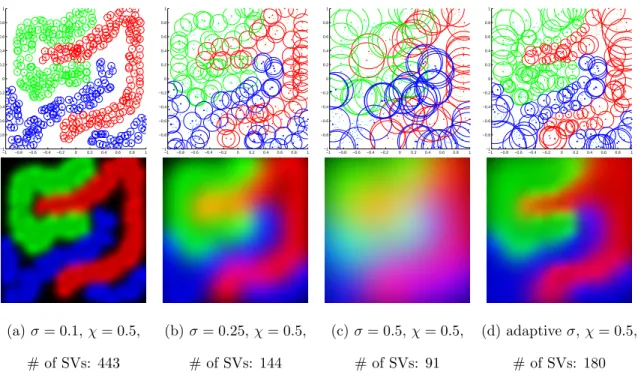
Figure 3.2: Visualization of the classification results for the “threeclass” dataset. Top row shows the selected support vectors with the corresponding σ values illustrated using circles. Bottom row shows the decision maps, which encode the output scores from the three one-class SVMs using red, green, and blue channels respectively. Both black color in (a-b) and orange/cyan/magenta colors in (b-c) indicate regions with ambiguities.

3.3

Adaptive Kernel Bandwidth

σ

As mentioned above, the adjustable kernel function used in STOCS contains a pa-rameter σ. We now discuss how to tune σi automatically and individually for each

support vector (xi, ωi, σi, χi). The core idea here is that a support vector should

not provide strong supports to negative examples, i.e., given a support vector xi,

we require k(xi, xn, σi) ≤ T for any negative example xn, where T is a constant

(39)

of the adjustable kernel function. That is, as soon as we meet a negative example

xn that yields k(xi, xn, σi) > T during the online learning, we update σi to ensure

k(xi, xn, σi) ≤ T. Since adjusting σ does not affect the score ordering among

ex-amples, the supports to previously seen negative examples can only decrease, which ensures the training process converges. It is also worth noting that for static datasets,

σi can be precomputed for each examplexi using the negative example xnthat yields

the largest k(xi, xn, σi) value.

Without losing generality, here we use the Gaussian kernel to illustrate the idea. For Gaussian kernel, the kernel bandwidthσis the standard deviation of the Gaussian function and controls the radius of the influence area of each support vector. As shown in Figure 3.2(a), when σ is too small, the obtained classifier can only recognize data that are close to one of the provided training examples, resulting over-fitting. On the other hand, large σ value causes fuzzy decision boundaries among different classes; see Figure 3.2(c). Hence, to ensure a proper σ value is used, previous approaches often rely on cross validation.

As shown in Figure 3.2(d), through automatically selecting different Gaussian support for different support vectors, the classifier obtained provides a sharp decision boundaries between the three training classes. which also output relatively few sup-port vectors. Demonstration of the effectiveness of self-tuning σ will be presented in Section 4.3.

(40)

−1 −0.8 −0.6 −0.4 −0.2 0 0.2 0.4 0.6 0.8 1 −1 −0.8 −0.6 −0.4 −0.2 0 0.2 0.4 0.6 0.8 1 (a)σ= 0.25,χ= 0.1, # of SVs: 398 −1 −0.8 −0.6 −0.4 −0.2 0 0.2 0.4 0.6 0.8 1 −1 −0.8 −0.6 −0.4 −0.2 0 0.2 0.4 0.6 0.8 1 (b)σ= 0.25,χ= 0.25, # of SVs: 236 −1 −0.8 −0.6 −0.4 −0.2 0 0.2 0.4 0.6 0.8 1 −1 −0.8 −0.6 −0.4 −0.2 0 0.2 0.4 0.6 0.8 1 (c)σ= 0.25,χ= 0.5, # of SVs: 205 −1 −0.8 −0.6 −0.4 −0.2 0 0.2 0.4 0.6 0.8 1 −1 −0.8 −0.6 −0.4 −0.2 0 0.2 0.4 0.6 0.8 1 (d)σ= 0.25, adaptive χ, # of SVs: 168 −1 −0.8 −0.6 −0.4 −0.2 0 0.2 0.4 0.6 0.8 1 −1 −0.8 −0.6 −0.4 −0.2 0 0.2 0.4 0.6 0.8 1 (e) adaptiveσ,χ= 0.1, # of SVs: 748 −1 −0.8 −0.6 −0.4 −0.2 0 0.2 0.4 0.6 0.8 1 −1 −0.8 −0.6 −0.4 −0.2 0 0.2 0.4 0.6 0.8 1 (f) adaptiveσ, χ= 0.25, # of SVs: 521 −1 −0.8 −0.6 −0.4 −0.2 0 0.2 0.4 0.6 0.8 1 −1 −0.8 −0.6 −0.4 −0.2 0 0.2 0.4 0.6 0.8 1 (g) adaptiveσ,χ= 0.5, # of SVs: 422 −1 −0.8 −0.6 −0.4 −0.2 0 0.2 0.4 0.6 0.8 1 −1 −0.8 −0.6 −0.4 −0.2 0 0.2 0.4 0.6 0.8 1 (h) adaptiveσ, adaptive χ, # of SVs: 385

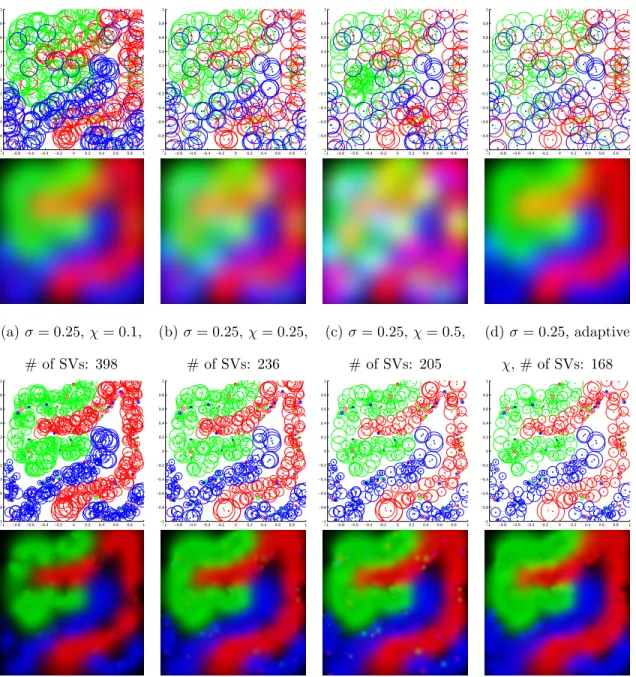
Figure 3.3: Visualization of the classification results when the dataset is corrupted with label noise, i.e., 5% of the random data have their labels changed. Under both fixed (a-d) and adaptive (e-h) Gaussian support situations, using adaptive cut-off values helps to limit the impacts of outliers.

(41)

3.4

Adaptive Cut-off Value

χ

The last standing parameter is the cut-off value χ, which is used to limit the effects of label noises (or outliers). When a training example (assuming it is mistakenly labeled) is observed, it may become a support vector with a large weight, yielding strong effect on final decision, resulting in that testing examples close to the outlier would be mislabeled. The cut-off χ is introduced to clamp weights of outliers and then limit their impact to classification. A large cut-off value cannot limit the effects of label noises, however, a small one may influence other correctly labeled support vectors. In STOCS, we adaptively select a cut-off value for each individual support vector.

Following the idea of tuning parameters for individual support vectors, here we also adaptively determine a proper χ value for each support vector. The key idea is that a support vector should have a higher χ if there are many positive examples within its support region and a smaller χ if there are many negative examples surrounding it. Hence we set:

χt = 0.5 + h+₍_x t)−h−(xt) 2(h+₍_x t) +h−(xt)) (3.4) where h+₍_x

t) and h−(xt) are the numbers of positive and negative examples that

satisfy k(xt, xi, σt) ≥ 0.6T, respectively. When h+(xt) > h−(xt), xt is surrounded

by more positive examples, thus xt is not an outlier and should have a large cut-off

value. When h+₍_x

t)< h−(xt),xt is surrounded by more negative examples, thus xt

is possibly an outlier and can have a small cut-off value, which limits the effects of

xt on the decision function. Note that h−(xt) ≥ 1 due to the way σt is calculated,

(42)

and Figure 3.3(c), which are generated using the same set of parameters, suggests that the presents of label noises can severely distort the decision boundaries. Using a smaller χvalues helps to reduce the impact of outliers, but at the expense of using more support vectors; see Figure 3.3(a-b). The use of adaptive σ also helps to limit the impact of outliers to their own neighborhoods; see Figure 3.3(e-g). Nevertheless, it does not fully address the problem.

As shown in Figure 3.3(d & h), using adaptive χ values can effectively limit the impacts of outliers. Note that, similar to σ, the χ values for different examples can also be precomputed when the dataset is static.

In summary, by assuming each support vector may have individual parameter settings, the three parameters, τ, σ, and χ, are successfully removed or adaptively tuned in online 1SVM training. Different from the original 1SVM training, our online 1SVM model of one class is trained using both positive and negative examples. We also achieve sharper decision boundary when training data contains label noise. In the next chapter, evaluations on our parameter self-tuning method are presented and comparisons with a benchmark method is also given.

(43)

Chapter 4

Experiments on Multiclass

Classification

Evaluations and experiments on multiclass classification are presented in this chapter to demonstrate the effectiveness of STOCS. We first evaluate the effectiveness of reweighting and parameter self-tuning by comparing STOCS with the conventional online 1SVM training technique [11]. Comparisons with the benchmark approach, the LIBSVM [9], for multiclass classification in terms of classification accuracy, support vector number, and training time, are then reported.

4.1

Datasets

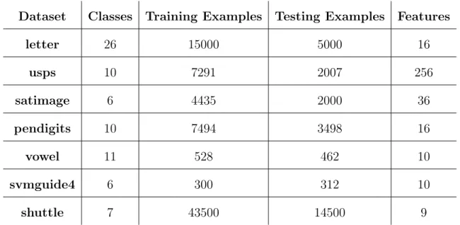
Table 4.1 summarizes information of datasets used in this chapter. All datasets can be downloaded fromhttp://www.csie.ntu.edu.tw/~cjlin/libsvmtools/datasets/. Here we give some details of several popular datasets. The “letter” dataset is created with gray images displaying the 26 capital letters in English alphabet, which is used

(44)

Dataset Classes Training Examples Testing Examples Features letter 26 15000 5000 16 usps 10 7291 2007 256 satimage 6 4435 2000 36 pendigits 10 7494 3498 16 vowel 11 528 462 10 svmguide4 6 300 312 10 shuttle 7 43500 14500 9

Table 4.1: Datasets used for multiclass classification

for letter recognition in machine learning. The “usps” and “pendigits” datasets are both created for handwritten digit recognition, which contain 10 numeric characters (from 0 to 9). The “shuttle” dataset contains 7 classes, in which approximately 80% of the data belongs to the first class. So the “shuttle” dataset can be used to demonstrate the effectiveness of classification algorithms when the distribution of training examples is distorted.

4.2

Effectiveness of Reweighting

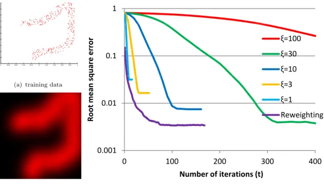
Figure 4.1 compares the convergence speed between the reweighting scheme (decay parameter is removed) and the conventional training approach under different decay rate settings. For the input dataset shown in Figure 4.1(a), we first generate a one-class SVM one-classifier using Equation (2.9) and (2.10) under fixed parameters (σ= 0.25;

(45)

−1 −0.8 −0.6 −0.4 −0.2 0 0.2 0.4 0.6 0.8 1 −1 −0.8 −0.6 −0.4 −0.2 0 0.2 0.4 0.6 0.8 1

(a) training data

(b) decision map 1 rro r ξ=100 0.1 q uar e e r ξ=30 ξ=10 0 01 m ean sq ξ=3 ξ=1 0.01 Root m ξ 1 Reweighting 0.001 0 100 200 300 400 Number of iterations (t) (c) convergence

Figure 4.1: Convergence of the conventional approach and the reweighting scheme. For a given set of examples (a), the decision map (b) obtained using the conventional approach under a very small decay rate is used as the ground truth. Comparing the decision maps generated after different iterations with the ground truth shows the convergence speeds of different approaches (c).

to generate a decision map (see Figure 4.1(b)), which is used as the ground truth. The decision maps obtained after different iterations and under different settings are compared with the ground truth. The results shown in Figure 4.1(c) suggest that the conventional approach generally converges after 10ξ iterations, i.e., τ < exp(−10). Furthermore, when a faster decay change rate is used, the final decision map defers from the ground truth, indicating a premature convergence. The classifier obtained using reweighting with the constant σ and χ setting yields almost identical decision map as Figure 4.1(b), but it converges much faster than the conventional approach

(46)

under ξ= 100.

4.3

Effectiveness of Parameter Self-tuning

0.05 0.1 0.15 40 60 80 100 sigma accuracy(%) letter 0.05 0.1 0.15 40 60 80 100 sigma accuracy(%) usps 0.05 0.1 0.15 40 60 80 100 sigma accuracy(%) satimage 0.05 0.1 0.15 40 60 80 100 sigma accuracy(%) pendigits 0.05 0.1 0.15 40 60 80 100 sigma accuracy(%) vowel 0.05 0.1 0.15 40 60 80 100 sigma accuracy(%) svmguide4 0.05 0.1 0.15 40 60 80 100 sigma accuracy(%) shuttle

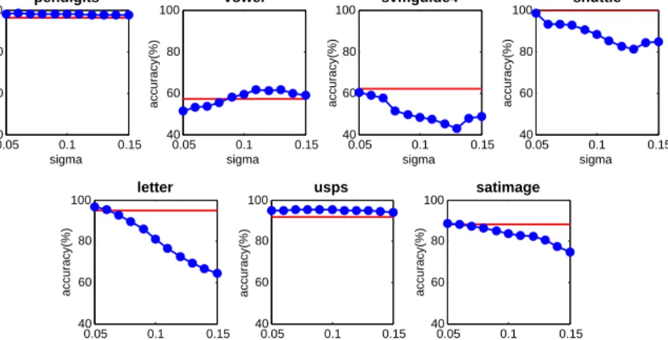
Figure 4.2: The effectiveness of self-tuning σ. Classification accuracy comparisons between self-tunedσ (red) and one-class SVM (blue) trained under different σ values are plotted.

We now evaluate the presented self-tuning scheme by comparing it with the con-ventional online one-class SVMs trained using fixed parameters. Datasets listed in Table 4.1 are used.

First we test the effectiveness of self-tuning σ using a Gaussian kernel and under a fixed cut-off value (χ= 0.5). Both STOCS and the conventional one-class SVM are trained using the training data and the classification accuracy on test data are mea-sured. To determine the properσ range for these datasets when using the traditional one-class SVM, we preform a coarse-to-fine grid search. Figure 4.2 plots the

(47)

classi-5 10 15 20 70 80 90 100 outlier ratio(%) accuracy(%) letter 5 10 15 20 70 80 90 100 outlier ratio(%) accuracy(%) usps 5 10 15 20 75 80 85 90 outlier ratio(%) accuracy(%) satimage 5 10 15 20 85 90 95 100 outlier ratio(%) accuracy(%) pendigits 5 10 15 20 20 40 60 80 100 outlier ratio(%) accuracy(%) vowel 5 10 15 20 0 20 40 60 outlier ratio(%) accuracy(%) svmguide4 5 10 15 20 70 80 90 100 outlier ratio(%) accuracy(%) shuttle

Figure 4.3: The effectiveness of self-tuningχ. Classification accuracy of self-tuned χ

(red), fixed χ = 0.1 (green), and fixed χ= 0.5 (blue) under increasing label noise is compared.

fication accuracy of the traditional one-class SVMs when σ varies within the proper range found. As expected, the performance highly depends on theσ value and there is no single σ value that works well for all datasets. STOCS adaptively selects σ for each support vector based on a fixed threshold value T = 0.25. Its performance is close to the traditional one-class SVM under optimal settings in all cases, and even outperforms the latter in the “svmguide4” and “shuttle” datasets. We attribute such performance gain to adjusting kernel bandwidth for support vectors individual, rather than using the same tuned parameters for all.

Next, we evaluated the effectiveness of self-tuning χ on datasets corrupted with label noises. For each dataset, we randomly and incrementally select training ex-amples as outliers and alter their labels. These outlier exex-amples with their original labels are then used as testing data to evaluate whether the classifiers can correct

(48)

labeling errors. The test is repeated 10 times for each dataset to compute the average accuracy. The results of self-tuning χ and fixed χare plotted in Figure 4.3, where σ

is self-tuned in all tests. The comparison clearly shows that the performance of con-ventional one-class SVM drops as the more label noise is introduced. Using self-tuned

χvalues not only improves the accuracy, but also makes the performance of classifier more stable.

4.4

Comparisons with LIBSVM

Finally we compare the performances of STOCS with a benchmark approach, the LIBSVM [9] using the one-vs-all approach, under both Gaussian and Linear kernels. We note in the passing that it is widely accepted (e.g. [52]) that for multiclass classifi-cation, one-vs-all is one of the simplest methods that almost always delivers the best performance. It is thus preferable to more complex methods including output coding schemes [20], [25] or single machine schemes [16]. This observation motivate us to concentrate on the following comparisons with the LIBSVM implementation of the on-vs-all approach, which is arguably the most widely used multiclass classification method in practice.

4.4.1

Gaussian Kernel

We start with comparing the performances of STOCS and LIBSVM on the afore-mentioned seven datasets under Gaussian kernel. For LIBSVM, both default and cross-validated parameter settings are tested. Note that here LIBSVM is tuned for each dataset individually, resulting different parameter settings for different datasets.

(49)

STOCS, on the other hand, uses the same self-tuning procedure with the threshold

T = 0.25 for all datasets.

60 80 100 sifi ca tion A ccu racy LIBSVM (default) LIBSVM (cross‐valid.) STOCS 20 40

letter usps satimage pendigits vowel svmguide4 shuttle

Cl as s STOCS 40 60 80 100 mpl e s sel e cted as SVs LIBSVM (default) LIBSVM (cross‐valid.) STOCS 0 20

letter usps satimage pendigits vowel svmguide4 shuttle

% of ex a STOCS

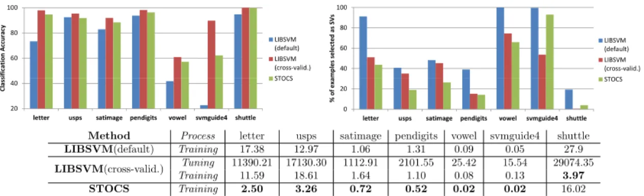
Method Process letter usps satimage pendigits vowel svmguide4 shuttle LIBSVM(default) Training 17.38 12.97 1.06 1.31 0.09 0.05 27.9 LIBSVM(cross-valid.) Tuning 11390.21 17130.30 1112.91 2101.55 25.42 15.54 29074.35

Training 11.59 18.61 1.64 1.10 0.08 0.13 3.97

STOCS Training 2.50 3.26 0.72 0.52 0.02 0.02 16.02

Figure 4.4: Comparison between STOCS and LIBSVM under Gaussian kernel. Top left shows the classification accuracy, top right shows the number of support vectors used, and bottom row gives the processing time needed.

Figure 4.4 shows that STOCS is more accurate than the LIBSVM under default settings in six out of the seven datasets. While LIBSVM with parameters tuned through cross-validation outperforms STOCS, the performance difference is less than 4% in six datasets. To achieve this performance gain, LIBSVM requires much longer processing time for parameter tuning. Furthermore, for most datasets, STOCS uses fewer support vectors than LIBSVM with both default and tuned parameters, allowing faster labeling of incoming examples.

4.4.2

Linear Kernel

To evaluate whether the presented approach works well for kernel functions that are not inherently adjustable, here we also compare STOCS with LIBSVM under linear

(50)

60 80 100 sif ic at io n A ccu ra cy LIBSVM (default) LIBSVM (cross‐valid.) STOCS 20 40

letter usps satimage pendigits vowel svmguide4 shuttle

Cl as s STOCS 40 60 80 100 mpl e s sel e cted as SVs LIBSVM (default) LIBSVM (cross‐valid.) STOCS 0 20

letter usps satimage pendigits vowel svmguide4 shuttle

% of ex a STOCS

Method Process letter usps satimage pendigits vowel svmguide4 shuttle LIBSVM(default) Training 9.72 8.13 1.11 1.07 0.13 0.06 16.5 LIBSVM(cross-valid.) _TrainingTuning 966.02_14.39 379.90_5.51 111.15_0.92 80.83_0.69 1.72_0.18 _1.312.87 14081.85_4.62

STOCS Training 2.09 6.65 1.17 0.41 0.02 0.01 9.28

Figure 4.5: Comparison between STOCS and LIBSVM under linear kernel.

kernel. To satisfy the nonnegative and normalized conditions that makes linear kernel normalized, we first map all examples feature-wise to range [0,1] and then normalize individual example vector to unit length. The same normalized datasets are used to train both LIBSVM and STOCS. However, LIBSVM uses the original linear kernel, whereas STOCS uses its adjustable version; see Equation 3.2. The same threshold valueT = 0.25 is used here for STOCS.

From Figure 4.5 we observe that, not only STOCS outperforms LIBSVM under the default parameter setting in all cases, it also outperforms LIBSVM with tuned parameters for two datasets and performs on par for two other datasets. This is remarkable since LIBSVM uses the best parameters specifically tuned for the given datasets.

4.4.3

Label Noise Handling

When the training data contains label noises, parameter tuning through cross-validation may cause the parameters being overfit to the corrupted data, leading to poor clas-sification accuracy. This is evidenced by Figure 4.6, where the LIBSVM with tuned

(51)

parameters is outperformed by the default parameters for “usps” and “satimage” datasets. Our approach, on the other hand, is robust against label noises and per-forms consistently. It outperper-forms LIBSVM with tuned parameters in four of the seven datasets. 60 80 100 si ficatio n ac cu ra cy LIBSVM (default) LIBSVM (cross‐valid.) STOCS 20 40

letter usps satimage pendigits vowel svmguide4 shuttle

Clas

s

Figure 4.6: Comparison with LIBSVM on training data corrupted by 10% label noises.

In summary, we have solved multiclass classification problems with STOCS. We evaluate and demonstrate the effectiveness of our proposed parameter self-tuning method step by step. Compared to the benchmark method LIBSVM, STOCS output shorter training time and fewer support vectors, while achieving comparable clas-sification accuracy with LIBSVM’s optimal parameter settings tuned for individual datasets. In the next chapter, online 1SVM learning is applied to solve binary classi-fication problems in computer vision to demonstrate its real-world application ability.

(52)

Chapter 5

Computer Vision Application

In the last chapter, we demonstrate the usefulness of applying STOCS to solve mul-ticlass classification problem. Here we show an application in computer vision, where STOCS is used to solve foreground segmentation and boundary matting for live videos. Foreground segmentation, a.k.a, video cutout, studies how to extract ob-jects of interest from input videos. It is a fundamental problem in computer vision and often serves as a pre-processing step for other video analysis tasks such as surveil-lance, teleconferencing, action recognition and retrieval. In the terminology of ma-chine learning, it belongs to binary classification problems. Given a frame of a video, foreground segmentation aims to determine a pixel belongs to the class of foreground object or background. Boundary matting aims for recovering the transparency and corresponding color along foreground objects [60]. It is one of the key techniques in film production applications, especially handling scenarios such as fuzzy object boundaries (e.g. hair) and motion blur. Over the years a significant amount of re-lated techniques have been proposed in both computer vision and machine learning

(53)

communities. However, some of them are limited to sequences captured by stationary cameras, while others require significant amount of training examples or cumbersome user interactions. Furthermore, most existing algorithms are rather complicated and computationally too demanding to be operated in real-time. As a result, there still lacks an efficient and powerful algorithm capable of processing challenging live video scenes with minimum user interactions.

(a) a separable case

(b) an inseparable case

Figure 5.1: Comparison between a binary SVM and two 1SVMs under two situa-tions. White circles and black dots represent the foreground and background training instances, respectively, while red dot denotes an unseen example. The straight line indicates the decision boundary of the binary SVM, whereas the ellipsoids show the boundaries of the two 1SVMs. In (a), binary SVM classifies the test example as fore-ground, whereas the 1SVMs labels it as unknown, since neither of the 1SVMs accepts it as inlier. In (b), binary SVM cannot confidently classify the test example since it is too close to the decision boundary, whereas 1SVMs is able to label it as background with confidence since only background 1SVM accepts it as inliner.

(54)

(a) input frame 0 (b) input stroke (c) after 1 itera-tion

(d) after 2 itera-tions

(e) after 3 itera-tions

(f) matting pixels

(g) after conver-gence

(h) matting pixels (i) binary segmen-tation

(j) composite (k) input frame 1 (l) initial label

(m) alpha matte (n) composite (o) input frame 104

(p) initial label (q) alpha matte (r) composite

Figure 5.2: Handling the “kim” sequence [14], which is challenging due to fuzzy object boundaries and camera motions. The user is only required to label the first frame (a) using strokes (b). Local classifiers are trained at each pixel location and then used to relabel the center pixel (c). Iterative training and relabeling leads to convergence (d, e, & g), even though ambiguous (grey) areas still exist. At each iteration, pixels along fore/background boundaries (non-cyan pixels in f & h) are detected, for which matting is performed. The final binary segmentation is computed through graph-cut optimization (i). Combining binary segmentation (i) with boundary matte (h) produces the full alpha matte, which is used to generate a blue screen composite (j). When new frames (k & o) arrive, they are initially labeled (l & p) using the classifiers trained by previous frames, before the same train-relabel-matting procedure takes place to produce the alpha mattes (m & q) and composites (n & r).

(55)

To fill that niche, this chapter applies the STOCS learning model introduced in Chapter 3 to solve the binary classification problem. Compared to the conven-tional binary SVMs, STOCS uses two online 1SVMs, which learn foreground and background distributions separately. We hypothesize that better performance can be achieved using two 1SVMs in the application. Here are the reasons: First, foreground and background may not be wel