An explainable sequence-based deep learning predictor with applications to song recommendation and text classification.

(1)

University of Louisville

ThinkIR: The University of Louisville's Institutional Repository

Electronic Theses and Dissertations

5-2019

An explainable sequence-based deep learning

predictor with applications to song

recommendation and text classification.

Khalil Damak

University of Louisville

Follow this and additional works at:

https://ir.library.louisville.edu/etd

Part of the

Computer Engineering Commons

, and the

Computer Sciences Commons

This Master's Thesis is brought to you for free and open access by ThinkIR: The University of Louisville's Institutional Repository. It has been accepted for inclusion in Electronic Theses and Dissertations by an authorized administrator of ThinkIR: The University of Louisville's Institutional Repository. This title appears here courtesy of the author, who has retained all other copyrights. For more information, please [email protected].

Recommended Citation

Damak, Khalil, "An explainable sequence-based deep learning predictor with applications to song recommendation and text classification." (2019).Electronic Theses and Dissertations.Paper 3164.

(2)

AN EXPLAINABLE SEQUENCE-BASED DEEP LEARNING PREDICTOR

WITH APPLICATIONS TO SONG RECOMMENDATION AND TEXT

CLASSIFICATION

By

Khalil Damak

B.E. Polytechnic Engineer, Tunisia Polytechnic School, 2017

A Thesis

Submitted to the Faculty of the

J.B. Speed School of Engineering

in Partial Fulfillment of the Requirements

for the Degree of

Master of Science in Computer Science

Department of Computer Engineering and Computer Science

University of Louisville

Louisville, Kentucky

(3)

(4)

(5)

AN EXPLAINABLE SEQUENCE-BASED DEEP LEARNING PREDICTOR

CLASSIFICATION

By

Khalil Damak

B.E. Polytechnic Engineer, Tunisia Polytechnic School, 2017

A Thesis Approved On

4/25/2017

Date

By the following Thesis Committee:

Olfa Nasraoui, Ph.D., Thesis Director

Hichem Frigui, Ph.D.

Gina Bertocci, Ph.D.

(6)

ACKNOWLEDGEMENTS

First and foremost, I would like to express my deepest gratitude to my supervisor Prof. Olfa Nasraoui for her constant guidance, her precious support and her valuable advice during all the steps of the project and beyond.

I would like to address my acknowledgements to Prof. Hichem Frigui, Prof. Gina Bertocci and Dr. Scott Sanders for accepting to serve in my thesis committee and for their valuable feedback and advice.

I would like to express my deep thanks to Prof. Gina Bertocci and Dr. Karen Bertocci for their valuable mentoring, encouragement and trust.

I address, likewise, my thanks to my lab-mates at the Knowledge Discovery & Web Mining lab for their support and friendship.

Last but not least, I would never forget the encouragement and the unconditional support I had from my parents, my brother, my friends and my beloved one.

(7)

ABSTRACT

AN EXPLAINABLE SEQUENCE-BASED DEEP LEARNING PREDICTOR WITH APPLICATIONS TO SONG RECOMMENDATION AND TEXT CLASSIFICATION

Khalil Damak April 25, 2019

Streaming applications are now the predominant tools for listening to music. What makes the success of such software is the availability of songs and especially their ability to provide users with relevant personalized recommendations. State of the art music recommender systems mainly rely on either Matrix factorization-based collaborative filtering approaches or deep learning archi-tectures. Deep learning models usually use metadata for content-based filtering or predict the next user interaction (listening to a song) using a memory-based deep learning structure that learns from temporal sequences of user actions. Despite advances in deep learning models for song recommen-dation systems, none has taken advantage of the sequential nature of songs by learning sequence models that are based on content. Aside from the importance of prediction accuracy in recom-mendation systems, recent research has unveiled the importance of other significant aspects such as explainability and solving the cold start problem where a new user or item with no prior history of interactions joins an online platform. In this work, we propose a hybrid deep learning structure, called “SeER”, that uses collaborative filtering and deep sequence models on the MIDI content of songs for recommendation. Our approach aims to take advantage of the superior capabilities of re-current neural networks, the multidimensional time series aspect of songs, and the power of matrix factorization to:

• provide more accurate personalized recommendations,

• solve the item cold start problem which is in the case of where a new unrated song is added to the set of choices to recommend; and

(8)

• generate a relevant explanation for a song recommendation using a novel explainability process we named “Segment Forward Propagation Explainability”.

Our evaluation experiments show promising results compared to state of the art baseline and hybrid song recommender systems in terms of ranking evaluation.

In addition, we demonstrate how our explanation mechanism can be used with generic sequential data beyond music, namely unstructured free text in two application domains: sentiment classification of online user reviews and delineating potential child abuse instances from medical examination reports.

(9)

LIST OF TABLES

TABLE Page

3.1 Normalized ratings of user 4 in the dataset. . . 30 3.2 Top 5 recommendations presented to user 4. The recommendations are sorted based

on the ratings predicted by the model and the explanations are represented by the start and end time of the 10-second sample inµs. . . 31 4.1 Hyperparameter tuning results: MAP@10 on the test data after training for 20 epochs.

The best results (in bold) are obtained, first, with 150 latent features and, then, with GRU. . . 39 4.2 Comparison of SeER with baseline recommender systems: Optimal MAP@10 results

within 20 epochs in 5 replicates. . . 41 4.3 Comparison of SeER with MM-LF-LIN [1] on an overlapping dataset. Our model’s

performance is assessed with MAP@500 after 20 epochs with 5 replicates. . . 43 4.4 Comparison of our preprocessing method consisting in the use of 16 channels with

the use of only the first channel. The performance is assessed with MAP@10 after 20 epochs with 5 replicates. . . 45

(12)

LIST OF FIGURES

FIGURE Page

2.1 An unrolled recurrent neural network representation (source: [2]) . . . 5

2.2 A LSTM cell representation . . . 5

2.3 A GRU cell representation . . . 7

2.4 An illustration of MF methods: R is the rating matrix and U and I are the user and item latent factor matrices. . . 10

3.1 Our dataset: the intersection between “The Lakh MIDI Dataset v0.1” and “The Echo Nest Taste Profile Subset” . . . 18

3.2 Play count visualization: (a) represents the box-plot statistics of the play count and (b) represents the density plot of the play count (without outliers for better visualization) 20 3.3 Mapping play counts into 5-star ratings . . . 21

3.4 MIDI to multidimensional time series transformation . . . 23

3.5 Box plot of the number of time steps in the transformed multidimensional time series 25 3.6 Time step normalization . . . 25

3.7 Song lookup matrix creation process . . . 26

3.8 Structure of SeER . . . 27

3.9 Sequence Forward Propagation Explainability process . . . 29

3.10 Explainability model . . . 30

3.11 Top 5 recommendations presented to user 4 in the web application. . . 31

3.12 Sentiment classification model . . . 32

4.1 ANOVA test on MAP@10 for the different models . . . 41

4.2 Tukey’s test on MAP@10 for pairwise comparison between the different models . . . 42

4.3 Evolution of the average (5 replicates) MAP@10 of all the models for 20 epochs . . 42 4.4 ANOVA test on MAP@10 for SeER trained with 16 channels and only the first channel 45

(13)

CHAPTER 1

INTRODUCTION

Machine Learning (ML) algorithms have proved useful and have become indispensable in numerous fields [3]. Their applications range from self driving cars to finance and health care. These algorithms sometimes help us make daily decisions while we may not even notice them. Such de-cisions include recommending which movie to watch, which product to buy or even which songs to listen to.

Thus, recommendation is becoming a common part of our daily lives. The ML systems that generate these personalized recommendations are called recommender systems [3]. These systems have known a tremendous and increasing interest by the ML research community during the last few decades. In fact, the quality of recommendations can sometimes contribute to the success of a company against the competition.

Among the fields in which recommendation is most decisive is music streaming. Music streaming platforms are the most natural way to listen to music today. The platforms are numer-ous: Spotify [4], Pandora [5], YouTube Music [6], SoundCloud [7] and many others. However, what makes the success of a platform over the other, aside from the availability of the songs, is its capacity to predict which song the user wants to listen to at the moment given their previous interactions.

Examples of challenges launched by actual streaming platforms emphasize the importance of recommendation to them. These challenges include the “RecSys challenge 2018” [8] that consisted of recommending songs for Spotify playlist continuation.

The most accurate recommender systems rely on complex black box machine learning mod-els that do not present any information related to how they output the predicted recommendation. This lack of transparency and inability to explain the decisions to human users may limit the

(14)

ef-fectiveness of these systems. In fact, one main challenge in recommendation today is designing a recommender system that mitigates the trade-off between explainability and prediction accuracy [9].

The most widely used techniques today in state of the art music recommender systems are Matrix factorization (MF)-based collaborative filtering approaches [10] and deep learning architec-tures [11]. Collaborative filtering recommender systems are based on the idea that people who agreed in evaluating an item in the past are likely to agree in the future [12]. Thus, similarities between users and items are used for recommendation. With MF [13], these similarities are obtained by factoring the rating matrix into user and item matrices in a latent space. For state of the art deep learning recommender systems, there are mainly two approaches. The first approach relies on content based filtering [14], meaning that it uses metadata to recommend songs given the similarity to items the user has liked in the past. Based on training data of the user’s feedback on items, item profiles are created and used to generate potential feedback for other items. The second approach uses sequence models to predict the next interaction (played song) given the previous interactions [15] [16] [17].

Despite the advances in deep learning for song recommendation and despite the sequential nature of songs that should make them naturally adapted to be used as inputs to sequence models, no work has used sequence models with the content of songs for recommendation.

Aside from accuracy and explainability, the cold start problem characterizes a significant issue that recommender systems [3], and especially collaborative filtering recommender systems, usually suffer from. The latter problem consists of generating recommendations for new users (user cold start) or recommending new items (item cold start) that are newly added to the system. In fact, most recommender systems need an initial history of interactions (ratings, clicks, plays...) to recommend. In music streaming platforms, new users and songs are constantly added making solv-ing this issue crucial.

1.1 Objectives

In this thesis, we take advantage of the sequential nature of songs, the prediction power of MF approaches for recommendation, and the superior capabilities of deep learning sequence models to achieve the following objectives:

(15)

• Propose a method to transform the Musical Instrument Digital Interface (MIDI) format [18] of songs into multidimentional time series to be used as input to deep learning sequence models and keep a large amount of information about the song;

• Integrate content based filtering using deep learning sequence models into collaborative filtering MF to build a novel hybrid model that provides accurate predictions compared to baseline recommender systems, solves the item cold start problem and provides an explanation to the recommendations;

• Propose a new type of explanation to song recommendation that consists of presenting to the user a short personalized MIDI segment of the song that characterizes the portion that the user is predicted to like the most; and

• Apply the proposed explanation method to sequence (text) classification.

1.2 Research questions

In order to evaluate our proposed methods, we aim to answer the following Research Ques-tions (RQs):

• RQ1: How does our model compare to baseline recommender systems?

• RQ2: How does our model compare to state of the art hybrid song recommender systems?

• RQ3: What is the importance of our use of the content data?

(16)

CHAPTER 2

BACKGROUND AND LITERATURE REVIEW

In this chapter, we state the techniques, algorithms and related work that we used as founda-tion or compared our methods to in this thesis. We start by defining deep learning sequence models and their various types and applications in Sec. 1. Then, in Sec. 2-3, we focus on recommender systems and state work that is most related to ours. In the sec. 4, we define two of the most relevant challenges in recommender systems that we try to remedy to being the cold start problem and transparency in recommendation. In Sec. 5, we present the evaluation metrics that we used to evaluate our model. Finally, in Sec. 6, we define the Musical Instrument Digital Interface (MIDI) format that we use in this thesis.

2.1 Deep learning sequence models

Sequence models, or Recurrent Neural Networks (RNNs), are a special form of Artificial Neural Networks that have the ability to span time steps in a dataset that includes instances which are related in time or space [19]. Such data includes text, videos and sounds. These types of models are used in multiple, sometimes creative, applications such as sentiment classification, machine translation, speech recognition and music generation [20].

An illustration of an unpacked RNN network is presented in Fig. 2.1.

The RNN cell takes as input at each time steptthe inputxtat the same time step and the

hidden state ht−1 from the previous time step. The hidden state being the output of the network

at each time step.

The hidden state is exploited differently depending on the application. For example in text classification, a dense layer with a Softmax or a Sigmoid function is added to the hidden layer of the last time step to predict the class.

The hidden state at a time steptis obtained with the following equation [19]:

(17)

Figure 2.1: An unrolled recurrent neural network representation (source: [2])

Figure 2.2: A LSTM cell representation

Here Whx and Whh are weight matrices and bh is a bias vector. They are the learnable

parameters of the model. Like conventional artificial neural networks, RNNs are trained with back-propagation [21].

In order to help capture longer and further dependencies in a sequence, updated and more complex RNN architectures emerged. The most important models are Long Short-Term Memory (LSTM) [22] and Gated Recurrent Unit (GRU) networks [23].

2.1.1 Long Short-Term Memory networks

LSTM is a type of RNNs that uses multiplicative gate units that learn to open and close access to the constant error flow [22]. With this process, LSTM networks are capable of learning long-term dependencies. An illustration of a LSTM cell is presented in Fig. 2.2.

(18)

to the next. A forget gate layer takes as inputxtandht−1and decides which information should be

removed from the cell state. The output of the forget gate layer being a vector of coefficients varying between 0 and 1, a multiplication with the cell state retains the amount of information characterized by these coefficients. Then, an input gate layer receives the same input as the forget gate layer and determines which information should be added to the cell state. Finally, an activation layer filters the cell state and decides which part of it should be output as the hidden stateht[2].

Hence, the hidden state at a time stept is obtained with the following equations [2]:

ht=ot∗tanh(Ct) (2.2) ot=σ(Wo[ht−1, xt] +b0) (2.3) Ct=ft∗Ct−1+it∗C˜t (2.4) ˜ Ct=tanh(Wc[ht−1, xt] +bc) (2.5) it=σ(Wi[ht−1, xt] +bi) (2.6) ft=σ(Wf[ht−1, xt] +bf) (2.7)

Where, ft andit∗C˜t are respectively the outputs of the forget and input gate layers; [., .]

is a concatenation; ∗ is an element-wise product and the Ws and bs are respectively weights and biases that will be learned when training the model.

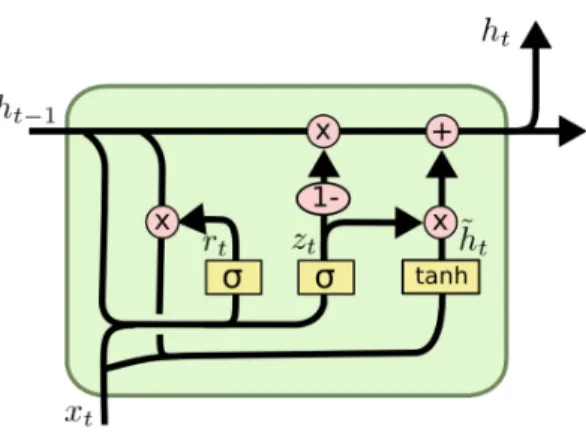
2.1.2 Gated Recurrent Unit networks

GRU can be seen as a simplified version of LSTM. In fact, the model merges the forget and input gate layers into an update gate layer and merges the cell state and hidden state [2] as presented in Fig. 2.3.

The hidden state at a time steptis obtained with the following equations [2]:

zt=σ(Wz[ht−1, xt]) (2.8)

rt=σ(Wr[ht−1, xt]) (2.9)

˜

ht=tanh(W[rt∗ht−1, xt]) (2.10)

(19)

Figure 2.3: A GRU cell representation

2.2 Recommender systems

Recommender systems are a type of information filtering systems [14]. In fact, recommender systems represent an extensive class of web applications that involve predicting user responses [24]. These systems are usually used to recommend items (that can be products, movies, songs, articles, etc.) that are relevant to the user. Recommender systems can be classified based on the past and current user information and input in addition to their structures [25] into five categories:

• Content-based filtering;

• Collaborative filtering;

• Knowledge Engineering or Rule-Based filtering;

• Demographic recommender systems; and

• Hybrids.

2.2.1 Content-Based filtering

Content-based filtering recommender systems recommend items given their similarity to items the user has liked in the past [26]. Based on training data of the users feedback on items, item and/or user profiles are created and used to generate potential feedback for other items. There are two different types of feedback:

• An Explicit feedback in which the user intentionally provides an opinion about the item by clicking, for example, on the like or dislike buttons or by rating an item by number of stars [26]; and

(20)

• An Implicit feedback in which information as whether the user viewed the item, finished reading the article or ordered a product is collected [26].

The item profile is a vector representation of the item given its features. If the item is, for example, a song, the features can be the artist, the genre, the year it was released etc. There are two approaches for recommending items to a user using item profiles. The first approach consists of creating a user profile, which is a vector representation of the users preferences with the same components as of the item profiles [24]. One way of building the user profile is to merge the item profiles, of the items rated by the user, weighted by the normalized ratings in the utility matrix. The normalization of the of the utilities consists of subtracting the average rating of the user. After normalization, items below the average rating will have a negative weight and items above the average will have a positive weight [24]. The items are, then, sorted by relevance to the user according to their similarity to the user profile. The second approach consists of using the item profiles as data points along with the ratings of a user as a target and training classification algorithms on the resulting data set. The trained model will then be used to predict the ratings of the user to other items. In this case, a model needs to be built for each user [24].

2.2.2 Collaborative filtering

Collaborative filtering is based on the idea that people who agreed in evaluating an item in the past are likely to agree in the future. Collaborative filtering may be classified into two categories according to the techniques they rely on. We find the Memory based and Model based techniques.

• Memory based collaborative filtering

The memory based collaborative filtering approach exploits similarities between ratings across a population of users by forming a weighted vote to predict unobserved ratings [27]. This approach can be divided into two main sections: user-item filtering and item-item filtering.

The user-item filtering, also known as User-based filtering [28], consists of finding users that are similar to the target user based on similarity in ratings. In order to compute the similarity between users, only items that both users rated are considered and similarity measures, such as cosine and Pearson, are applied [28]. Finally, missing ratings are determined via weighted aggregations of the ratings from a number of most similar users.

The item-item approach, also known as item-based filtering [29], takes as input an item, finds users who liked that item and recommends other items that those users are or similar users

(21)

also liked. Technically, the item-based approach recommends items based on their similarity with other items that the target user rated [29]. Thus, this filtering technique is similar to the user-based approach except that the similarity is computed between items instead of users and the aggregation of the ratings is determined using a number of most similar items.

• Model based collaborative filtering

In Model based collaborative filtering, models are developed using machine learning algo-rithms to predict users ratings of unrated items. This approach learns and fits a parametrized model to the utility matrix and uses it to provide recommendations [10]. The algorithms in this approach can be broken into 3 sub-types being: Clustering based algorithms, Matrix factorization based algorithms and Deep learning approach.

In our work, we focus on both Matrix factorization and deep learning approaches based on sequence models. We will present both these models in depth in future sections.

2.2.3 Knowledge Engineering or Rule-Based filtering

Rule-based filtering relies on an expert system style where the user answers a set of questions derived from a decision tree and, according to the answers, receives a list of relevant products [25].

2.2.4 Demographic recommender systems

In Demographic recommender systems, the items are recommended to the users based on their demographic attributes (age, gender, location, ) instead of their behavior [25]. The recom-mender systems can be either based on handcrafted stereotypes or on Machine Learning techniques by classifying users into classes based on their demographic attributes [25].

2.2.5 Hybrid recommender systems

Hybrid recommender systems combine several recommendation strategies in the aim of pro-viding better results by combining the strengths of the individual methods and circumventing their weaknesses [25]. Hybrids can be categorized into two families given the fact that they whether combine the input data sources or the recommendation strategies [25]. The second family of hybrid recommenders can further be categorized by the way they combine the recommendation strate-gies [25]. In fact, stratestrate-gies can be combined in either a parallel or a sequential order [25].

(22)

Figure 2.4: An illustration of MF methods: R is the rating matrix and U and I are the user and item latent factor matrices.

2.3 Related work in recommender systems

As we will see in the following chapter, our model is a hybrid song recommender system that can be seen as a combination of Matrix Factorization (MF) and deep learning sequence models. Hence, in this section, we will present the works that are related to ours based on these characteristics. We will start by presenting MF and deep learning sequence models in recommendation. Then, we will focus on hybrid music recommender systems.

2.3.1 Matrix factorization in recommendation

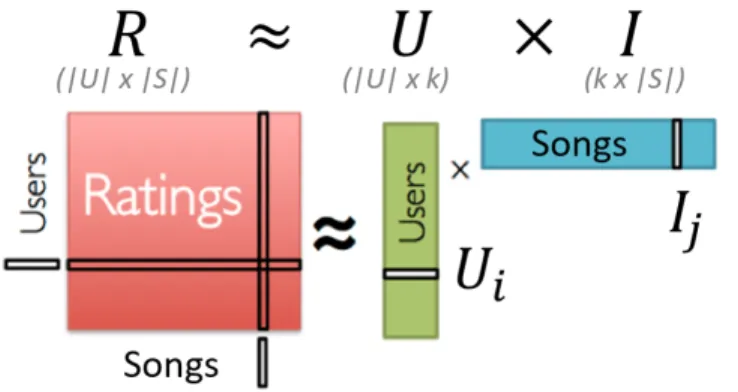
Matrix factorization consists, in its basic form, of characterizing both the items and the users by vectors of factors inferred from item rating patterns [13]. These factors are called latent factors and represent hidden characteristics of the users and items. A user i is represented by a vector of preferences of factorsUi and an item j is represented by a vectorIj where each element

expresses how much the item exhibits each factor [30]. The factorization models can be formulated as optimization problems with objective functions and constraints [10].

An illustration of MF is presented in Fig. 2.4.

The multiplication of the user and item latent matrices yields an approximate reconstructed rating matrix. Unlike the real rating matrix which is sparse, the reconstructed rating matrix does not have any missing value. Thus, the rating of each user to each item can be predicted.

The matrix factorization techniques for recommender systems include Principal Component Analysis (PCA), Singular Value Decomposition (SVD), Probabilistic Matrix Factorization (PMF) and Non-Negative Matrix Factorization (NMF).

(23)

PCA is a statistical method aiming to find patterns in high dimensional data sets [31]. It is a powerful technique of dimensionality reduction and realization of the MF approach [31]. In collaborative filtering, PCA is applied to the rating matrix of users to items. It allows to obtain an ordered list of components that account for the largest amount of the variance from the data in terms of least squared errors [31].

• Singular Value Decomposition

SVD reduces the dimensionality of the utility matrix and generates low rank matrix approx-imations which represent the latent features of users and items [10]. In fact, aM×N rating matrix

Ris represented as follows:

R=U SVT (2.12)

Where, U and V are respectively M ×M and N ×N orthogonal matrices and S is an

M×N singular orthogonal matrix with non-negative elements [31]. The diagonal elements inS are called the singular values of matrixS [31] and are usually placed in the descending order of their magnitude [10]. SVD realizes the decomposition by minimizing its reconstruction error as follows:

min

U,S,V

X

(i,j)R

(Rij−[U SVT]ij)2 (2.13)

By ignoring the small singular values, the dimensions of the matrices are reduced toklatent factors [10].

• Probabilistic Matrix Factorization

PFM treats ratings as a probabilistic graphical model and provides a probabilistic approach using Gaussian distribution noise on the known data and the factor matrices [10]. For a rating value of a userifor a moviej Rij, k-dimensional user-specific and movie-specific latent feature vectors are

respectively represented by Ui and Vj [31]. The conditional distribution over the observed ratings

RRN×M and the prior distributionsU Rk×N andV Rk×M given by [31]:

p(R|U, V, σ2) = N Y i=1 M Y j=1 [N(Rij|UiTVj, σ2)]Iij (2.14) p(U|σ2_U) = N Y i=1 N(Ui|0, σ2UI) (2.15)

(24)

p(V|σ2_V) =

M

Y

j=1

N(Vj|0, σV2I) (2.16)

Where,N(x|µ, σ2) denotes the Gaussian distribution with meanµ and varianceσ2 andIij

denotes the indicator variable that is equal to 1 if userirated itemj and 0 otherwise.

• Non-negative Matrix Factorization

NMF is a matrix factorization technique that imposes constraints of non-negativity on factor matrices [10]. This technique can be expressed as an optimization problem as follows:

min

U,I kR−U Ik 2

F (2.17)

WhereU RM xK andIRkxN are respectively the latent matrices of the users and items and

R_RM xN _{is the rating matrix. All of the matrices should only contain non-negative values.}

NMF can only find a local minimum of the error as the problem is nonconvex. However, it can be minimized by a simple multiplicative form as follows:

     Iij=Iij (UT_R₎ ij (UT_{U I}₎ ij Uij =Uij (RIT)ij (RIIT₎_ij (2.18) Hence, the solution is reached by iterating until convergence.

2.3.2 Deep learning sequence models in recommendation

Various recommender systems rely on sequence models. However, not all of them use them for recommendation with user identification. In fact, some models are session-based, meaning that they only recommend based on short-term interests [15] [16] [17]. These methods take the data as a sequence of interactions, clicks or songs for instance, and predict the next interaction. They are collaborative filtering methods and, so, do not use any side information. Other methods introduce content into session-based recommendation [32] [33] and prove that side information enhances the recommendation quality [11].

Other recommender systems using RNNs took into consideration user identification [34] [35]. These engines use RNNs to model temporal dependencies for both users and movies [34] [35] and generate reviews [35]. The main objective of these models is to predict ratings of users to items using seasonal evolutions of items and user preferences in addition to user and item latent vectors. Alternate models considering user identification and using RNNs aimed to generate review tips [36],

(25)

predict the returning time of users and predict items [37] or produce next item recommendations for a user by proposing a novel Gated Recurrent Unit (GRU) structure [38].

Finally, recommender systems also use RNNs as a feature representation learning tool [11]. These models apply RNNs on content data instead of on the sequence of interactions as in the aforementioned recommender systems. Among the related works, we count [39], which is a multi-task learning model that uses RNNs to create a latent representation of items that will be used as input to a collaborative filtering model with a learnable user embedding to predict ratings. The RNN takes as input a sequential representation of the item and is trained on an alternate objective, such as tag recommendation, to create the item latent representation.

2.3.3 Hybrid music recommender systems

Song recommendation received contributions from several approaches. Hybrid methods need both content features and ratings. In song recommendation specifically, the works often diverge in terms of input data used and features created. In fact, music items can be represented by features derived from the audio signal, social tags or web content [40].

Among the most noticeable hybrid song recommender systems, [41] learns collaborative filtering latent factors of users and items using matrix factorization and sums their product with the product obtained with created user and song features. The song features are created by generating spectrograms of 5 second samples of songs and converting them to features using PCA.

[42] formulates the song recommendation problem as a song inclusion in playlists problem. It consists of combining non-negative matrix factorization with graph regularization. The playlist and song graphs are based on high level, social, temporal and metadata features. [1] learns artist embeddings from biographies and track embeddings from audio signals using convolutional neural networks on spectrograms. These embeddings are later aggregated and multiplied by user latent factors obtained by weighted matrix factorization to get the ratings.

Finally, [43] relies on the moods of the artists songs in addition to audio content for rec-ommendation. The system positions the users in a mood space, given their favorite artists, and recommends new artists for them using similarity measures.

2.4 Challenges in recommendation

In this section, we discuss two major challenges in recommender systems that are the cold start problem and the lack of transparency.

(26)

2.4.1 The cold start problem

The cold-start problem is a notorious problem for collaborative filtering recommender sys-tems [3]. It happens when recommendations have to be made for new users in the system, this problem is called user cold start, or when new items that no one has rated yet need to be recom-mended [3]. The latter problem is called item cold start.

One possible solution to the cold-start problem is to use user and item features because they can “help create a bridge between existing users or items and new users or items” [3].

In our model, as we will see in the next chapter, we rely on song attributes to solve the item cold start problem.

2.4.2 The lack of transparency: Explainability in recommender systems

The most powerful recommender systems are black box models. This means that they do not tell any information about how the predictions are made. This lack of transparency results into users not trusting the suggested recommendations [3].

State of the art works tried to present explanations to the recommendations in order to remediate to this issue. The types of explanations vary with the different approaches. According to [44], these approaches can be categorized in three different types:

• Neighbor Style Explanation: Relying on the user’s neighbors’ ratings of the recommended item, a histogram of these ratings (or a categorization: bad, neutral and good) is presented to the user as an explanation [3].

• Influence style Explanation: A table of the items that had the highest impact in generating the recommendation is presented as an explanation [3].

• Keyword style Explanation: Matching words are presented as explanations and are deter-mined by analyzing the content of the recommended item and the user profile [3].

Our explainability method, that we will be presenting in the following chapter, consists of a 10-second MIDI segment of the song having the highest impact in generating the recommendation. Thus, our explainability method can be seen as an influence style explanation.

(27)

2.5 Recommendation evaluation

We present two ways of evaluating a recommender system’s performance which are rating prediction and recommendation ranking evaluation.

2.5.1 Rating prediction evaluation

The rating prediction is evaluated using the two evaluation metrics presented below. These metrics compute distances between the true ratings of user ito itemj Rij and the predicted ones

ˆ

Rij. The lower the values of these metrics is, the better the prediction is.

• Root Mean Square Error (RMSE)

RM SE(model) = v u u t 1 |R| X (u,i)R ( ˆRui−Rui)2 (2.19)

• Mean Absolute Error (MAE)

M AE(model) = 1

|R| X

(u,i)R

|Rˆui−Rui| (2.20)

2.5.2 Recommendation ranking evaluation

In order to evaluate the recommendation ranking, we use Mean Average Precision (MAP) at cutoff K (MAP@K). This metric evaluates the ranking of the top K recommended items for each user averaged over all the users. The MAP@K formula is presented below:

M AP@K(model) = 1 |U| |U| X u=1 1 mu K X k=1 Pu(k).relu(k) (2.21) Here,

• |U|is the number of users in the testing set;

• mu is the number of items rated by the useruas relevant. In our case, as we will see in the

next chapter, we created normalized ratings and considered an item as relevant to a user if the rating is greater than or equal to 3;

• Pu(k) is the precision at cutoff K, which is the precision calculated by considering only the

subset of recommendations from rank 1 through k;

Pu(k) =

#relevant recommendations in the subset1through k

(28)

• relu(k) is the indicator of relevance such that: relu(k) =     

1if recommended item k is relevant

0otherwise

(2.23)

2.6 Musical Instrument Digital Interface (MIDI)

MIDI is a technical standard allowing to connect devices that make and control sound, such as synthesizers, samplers, and computers, so that they can communicate with each other, using MIDI messages [18]. Technically, MIDI involves a communication protocol, a digital interface and electrical connectors [45]. This technical standard allows “easy note editing, flexible orchestration, and song arrangement” [18].

MIDI files are polyphonic digital instrumental audios. They are usually used in karaokes. They are constituted of event messages that are consecutive in time. Each event message includes the following attributes:

• Notation: the notes played;

• Pitch: how high or low the note played is;

• Velocity: how rapidly and forcefully a note, as in a keyboard key, is pressed;

• Vibrato: a regular, pulsating change of pitch;

• Panning: a distribution of a sound signal into a new stereo sound field; and

• Clock signals: signals that set the tempo.

These events are distributed over 16 possible and available channels of information. A channel is an independent path over which messages travel to their destination [18]. Each channel can be programmed to play one instrument. Thus, a MIDI file can play up to 16 instruments simultaneously.

(29)

CHAPTER 3

AN EXPLAINABLE SEQUENCE-BASED DEEP LEARNING PREDICTOR

CLASSIFICATION

In this chapter, we present our methods. We start by describing the data that we used along with its preparation procedure. Then, we present our model, which is an explainable hybrid song recommender system entitled “SeER”. This being done, we describe our explainability pro-cess called “Segment Forward propagation”. Within the last subsection, we present an application of our explainability process in sequence classification tasks beyond music data, namely for text classification.

3.1 Data preparation

In this section, we start by presenting the data that we used. Then, we describe the prepro-cessing steps that we applied to it.

3.1.1 Data used

Our recommender system is hybrid, meaning that it uses several modalities of the data. It combines both MF and content based filtering. Thus, it needs as input both user to item ratings and content. The Million Song Dataset (MSD) [46] is a public collection of audio features and metadata for a million contemporary popular music tracks [46].

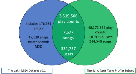
The MSD also comprises a number of complementary datasets contributed by the community. These datasets overlap with the MSD in terms of the songs they include. In our project, we used two of these datasets that include both the types of data that we need: “The Echo Nest Taste Profile Subset” [47] and “The Lakh MIDI Dataset v0.1” [48].

• The Echo Nest Taste Profile Subset

(30)

Figure 3.1: Our dataset: the intersection between “The Lakh MIDI Dataset v0.1” and “The Echo Nest Taste Profile Subset”

[47]. It includes user-song-play count triplets collected from The Echo Nest’s undisclosed partners. The dataset comprises 1,019,318 unique users, 384,546 unique MSD songs and 48,373,586 play counts. The play count being the number of times a user played a song. The dataset is filtered in a way that each user interacted with at least 10 different songs.

• The Lakh MIDI Dataset v0.1

The Lakh MIDI Dataset is a collection of 176,581 unique MIDI files of which 45,129 are matched to MSD songs [49]. The matching of the MIDI files to the actual songs was done by, first, developing “series of efficient learning-based methods” to discard the vast majority of pos-sible matches and, then, “dynamic time warping-based MIDI-to-audio alignment” to compare the remaining entries [48].

Technically, the dataset comes with a list of matching scores for each MIDI file to songs from the MSD. We relied on the highest matching score for each MIDI file to match the Lakh MIDI dataset to the MSD.

• Our multimodal (usage and content) dataset

In order to create our multimodal dataset, we combined both “The Echo Nest Taste Profile Subset” and “The Lakh MIDI Dataset v0.1” by taking the intersection in terms of songs. As a result, we obtained a dataset with 331,737 users, 7,677 songs in both play count triplets (usage data) and MIDI files (content data) and 3,519,506 play counts. An illustration of the dataset creation is presented in Fig. 3.1.

(31)

3.1.2 Data preparation

In order to prepare the data to be used as input to our model, obtain unbiased results, and fasten the training, we needed to prepare our dataset. In this section, we describe the data preparation steps.

• Mapping the play counts into ratings

Depending on its output, a model-based recommender system can be assimilated to a re-gression model or a classification model. In the case where it is assimilated to a classification model, the output is binary. [50] used movie rating datasets and transformed the rating matrix into an interaction matrix that takes 1 if the user rated the movie and 0 if not. In movie recommendation, a user rating a movie means that they watched it (interacted with it). However, in song recommen-dation, the interactions alone are not sufficient. In fact, because of the shortness of songs compared to movies, there can be many non-significant interactions. In fact, if a user interacts with a movie, they know at least what it is about, what its genre is or who the actors are. Because watching a movie is time-consuming, we can assume that the user showed at least some interest to it before watching it. This is not the case in music. Because a song can be recommended to a user after a sequence of songs, the user can listen to it without genuine interest. Thus, unlike movies, a song that has been listened to once does not necessarily mean that the user is interested in it.

One solution to this issue could be to consider the play count as an interaction if it is higher than 2 or 3. However, it is clear that the more a song is listened to, the more it is liked by the user, and this information cannot be captured by interactions alone.

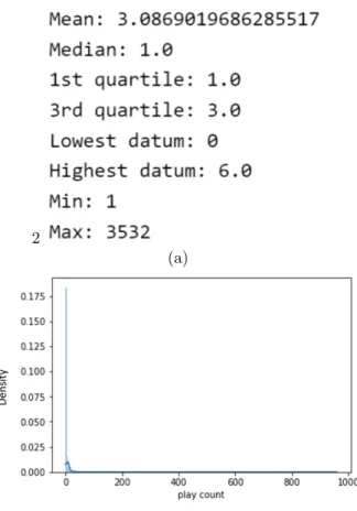
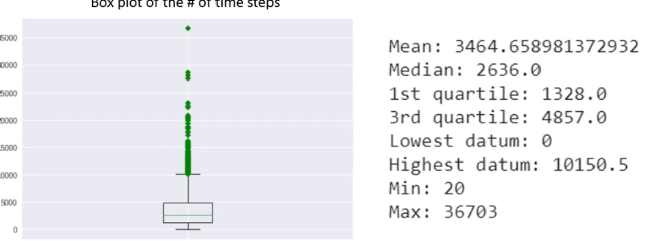
Fig. 3.2 shows the box-plot statistics of the play count and its distribution after removing the outliers. We did not remove the outliers for the study. We just removed them to plot the distribution for better visualization.

From the box-plot statistics and the density plot, we notice that the play count follows a power law distribution with a median of 1. Thus, at least half of the play counts are one. Hence, if we had used the play counts as interactions, at least half of them may have been wrongly interpreted. Hence, one solution is to assimilate our problem to regression. In this case, the target needs to be continuous. We have two options, whether to use the play counts directly as a target or to transform them into pseudo-ratings.

From Fig. 3.2 (b), we notice that there are users that listened to the same song hundreds and thousands of times. In fact, in Fig. 3.2 (a), we see that the maximum play count is 3,532. These

(32)

2

(a)

(b)

Figure 3.2: Play count visualization: (a) represents the box-plot statistics of the play count and (b) represents the density plot of the play count (without outliers for better visualization)

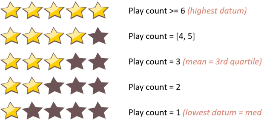
high play counts are outliers that may bias our results and make training the model to predict the play count harder. In fact, it is true that the more a song is listened to by a user, the more likely that the user likes it. However, if a user listens to a song 10 or 3,000 times, it is clear that they like it and both cases should be considered the same. With these observations, we proved the need to normalize our play counts. To do so, we used the most common scale of 5 ratings and obtained normalized ratings using the box plot as follows:

• As we discussed earlier in this subsection, a play count that is equal to 1 most likely means that the user does not show any interest in the song. Thus, we converted play counts of 1 into ratings of 1 star.

• We assumed that a play count of 2 most likely means that either the user tried to listen to the song twice and did not like it much or that the song was recommended twice to the user and they listened to it unintentionally. Hence, we converted play counts of 2 into ratings of two stars.

(33)

Figure 3.3: Mapping play counts into 5-star ratings

• The play count of 3 is the average. Thus, we converted it to the average rating which is three stars.

• We assumed that if a user listened to a song 6 times or more, then, that user likes the song a lot. We made this assumption based on the box-plot statistics where 6 is the highest datum.

• Finally, we assumed that the remaining play counts of 4 and 5 mean that the user likes the song to a certain extent. Hence, we converted these play counts to the remaining rating which is 4 stars.

The play count normalization process is illustrated in Fig. 3.3.

• Removing users with less than 20 interactions

Our actual dataset has a sparsity of 99.86%. This kind of highly sparse data is common in recommender system applications. However, the sparser the data, the harder the model tends to learn. Thus, reducing the data sparsity may improve our model’s performance. Moreover, training a deep learning model on large datasets takes a lot of time. So, it is also better to reduce the size of the dataset in order to reduce the training time.

One of the most used datasets in collaborative filtering is the “MovieLens” dataset [51]. This dataset includes 1,000,209 ratings of 6,040 users to 3,706 movies, hence having a sparsity of 95.53%. Only the users that have interactions with at least 20 distinct movies were kept. [50] used, in addition to the MovieLens dataset, another dataset of user to movie ratings called Pinterest. This dataset has a higher sparsity than the MovieLens or our dataset. The authors reduced its size and sparsity by removing the users that have fewer than 20 unique interactions.

(34)

For our data, we followed the same methodology used in [50]. Hence, we removed the users that interacted with fewer than 20 unique songs. We ended up with a dataset that has 941,044 normalized ratings of 32,180 users to 6,442 songs. We reduced the sparsity of our dataset to 99.54%. Also, we still kept a high number of interactions that is close to the number of interactions in the MovieLens dataset.

• Transforming the MIDI files into multidimensional time series

We needed to create a multidimensional time series representation of the MIDI files in order to input them to sequence models. In fact, our objective was to represent the evolution of the MIDI audio throughout time. So, we looked for a way to extract the different notes with the way they are played in the file throughout time.

To do so, we first used “MIDICSV” [52], which is a program that translates “MIDI music files into a human- and computer-readable CSV (Comma-Separated Value) format” [52]. The converted CSV sheet comprises successive events in the rows. Each event has the following features:

• Track: The audio in the MIDI file can be divided into a certain number of tracks that delineate segments with similar characteristics for example. A MIDI file may include a large number of tracks. Having all the notes in different tracks or in the same track does not change anything in its musical content. In fact, segmenting a MIDI into various tracks simplifies updating the file after recording. For example, it is easier to change the velocity of just the drums track if it is too loud [53].

• Time: The value of the time at which the event happens in the MIDI file differs from the absolute time in the song. In fact, the time in a MIDI file is measured in pulses, or beats, and depends on the tempo, which is a measure of speed of the music segment, and the division of the section of the song, which is the number of pulses per quarter note, in order to be perceived as absolute time. The following equation shows the conversion of MIDI time into absolute time:

absolute time[µs] = M IDI time[pulses]

Division[pulses/quarter note]T empo[µs/quarter note] (3.1)

• Type: The type of the event can be either Note on c (start playing the note), Note off c (stop playing the note), Pitch bend c (vary the pitch), Control c (assign a control, such as sustain

(35)

Figure 3.4: MIDI to multidimensional time series transformation

or reverbation, to a channel) or Program c (assign the instrument to be played by a channel). There are 128 possible instruments that can be emulated by a MIDI file.

• Channel: The channel means to which of the 16 channels the event is going to be assigned. For example if the type is a note on C and the channel is 1, then, the specified note will be played on channel 1.

• Note: The note specifies which note is going to be played if the type is note on C or stopped if the type is note off C. This feature can take 128 possible values (from 0 to 127) with note number 60 being middle C [52]. A value of 0 is equivalent to a note off C.

• Velocity: This feature specifies the velocity of the note played if the type is note on C. For our preprocessing, we only focused on the notes played throughout time. Thus, we only considered the “Note on C” events. Also, we considered all the sequences of notes played in the MIDI file within the 16 possible channels and, so, instruments that can be played simultaneously. However, we did not consider the 128 possible instruments themselves as features because of two main reasons. First, the MIDI file can only play up to 16 instruments. So, at least 112 columns will be empty and the multidimensional time series will be sparse and sequences of zeros will most likely bias and slow down the training. Also, we are not interested in the instruments themselves but in the sequences of notes and the harmony within the different instruments.

Furthermore, we saved the velocity of each note in order to capture the way they were played. Hence, each transformed multidimensional time series is constituted of a certain number of rows representing the number of “Note on C” events and 32 features representing the notes and velocities played within the 16 channels.

(36)

• Normalizing the number of time steps

We transformed each of the 6,442 MIDI files that are in our dataset into multidimensional time series. Depending on the duration of the audio and its number of notes, the number of time steps varies from transformed time series to another. Although sequence models can handle variation in time steps for the different training instances, they cannot train batches with different lengths. In fact, training a deep learning model with mini-batch gradient descent is the most popular practice [54] that allows relatively fast convergence of the objective function.

Mini-batch gradient descent [55] compromises between Stochastic Gradient Descent (SGD) [56] and batch gradient descent in terms of memory, training time and noisiness. Batch gradient descent computes the gradient of the cost function with respect to the parameters of the model for the entire training dataset [54]. The process can be time consuming and intractable for datasets that do not fit in memory [54]. Moreover, the batch gradient trajectory may land in a saddle point, which is a local minimum from which it cannot escape. On the other hand, SGD performs a parameter update for each training example [54]. SGD’s fluctuation allows it to solve the saddle point issue of batch gradient descent and enables it to jump to new and potentially better local minima [54]. However, SGD’s disadvantage is its inefficiency by having to loop over the entire dataset many times to find a good solution.

Mini-batch gradient descent has the advantages of both techniques and performs an update for every mini-batch of n training examples. This way, it reduces the variance of the parameter updates which can lead to more stable convergence [54] and makes the training for each epoch faster.

Given the advantages of mini-batch gradient descent as an optimization technique, we de-cided to train our model with batches. In order to train a sequence model with batches, the training instances need to have the same length, in other words, the same number of time steps. Thus, we normalized the different multidimensional time series to the same number of time steps.

For that, we relied on the box plot of the number of time steps in addition to empirical observations. The box plot of the number of time steps in presented in Fig. 3.5.

Our objective is to keep as much information as possible from all the songs, avoid over-padding multiple instances and reduce the data size in a way to avoid memory errors. We can notice that half the songs have at least around 2,600 time steps, which is close to the average number of time steps (around 3,400). Also, at most, 25% of the songs have less than 1,328 time steps. So, if we normalize to the median (2,600), around 25% of the songs will have more padding zeros than notes.

(37)

Figure 3.5: Box plot of the number of time steps in the transformed multidimensional time series

Figure 3.6: Time step normalization

Thus, we decided not to normalize to a number of time steps higher than the median. Moreover, at least 75% of the songs have more than 5,200 time steps (which is the double of the median). Hence, if we normalize to the median, at least 75% of the instances will keep at least 50% of their notes. Furthermore, even when we tried to increase the normalization number of time steps, we ended up with either a memory error or a very slow training.

Given the above reasons, we decided to normalize the transformed multidimensional time series to 2,600 time steps. The normalization process is illustrated in Fig. 3.6.

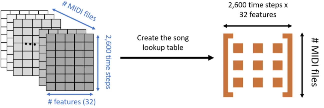
• Creating the song lookup matrix

Our target variable is the user to song rating vector. Hence a model to be trained should receive simultaneously, for each rating, user and item inputs. If we organize our input in the order of the ratings, we would have 941,044 (number of ratings) item inputs. Each of the inputs is an array of 32 features and 2,600 time steps making the input too large to fit in the memory. Furthermore,

(38)

Figure 3.7: Song lookup matrix creation process

the input in this case includes many duplicate song arrays characterizing the same song in different ratings. This redundancy makes the input memory inefficient and leaves room for optimization. Our solution to this issue is to flatten the song arrays and create a lookup table that includes all of the song contents. For each rating, the row related to the song in question can be extracted, reshaped to a two dimensional array and used to train the model.

The aforementioned transformation process is presented in Fig. 3.7.

3.2 SeER: Sequence-based Explainable Recommender System

Our initial objective was to build a recommender system that combines the power of Ma-trix factorization and deep learning sequence models in order to generate accurate and explainable recommendations. Three main observations inspired the design of our model:

• First, songs present an evolution in time. Thus, sequential patterns in the content of songs can be determined and used to help improve the recommendation performance. On the other hand, deep learning sequence models are the most adequate models in learning sequential data. Given those reasons, we decided to investigate the content of songs by relying on MIDI data and integrating a sequence model component to represent the songs.

• Also, in MF-based models, the users and items are both represented by latent factor matrices that are learned by training the model given the true ratings. The number of latent factors being chosen by the user. We noticed that the hidden states, which are the outputs of sequence models, are both learnable by training the cells and of chosen size. These two characteristics are the basic properties of an embedding matrix. For these reasons, we thought about assimilating

(39)

Figure 3.8: Structure of SeER the output of sequence models to the user latent factor matrix.

• Finally, explaining a prediction consists of determining the reason why the result was obtained. This may be realized by finding the most important portion of the instance that helps explain the prediction. For example, in image classification, if a picture was predicted to have a car, one way of explaining the reason can be to present the portion of the picture containing the wheel or the headlight. In our case, we thought about explaining song recommendations by providing the user with the segment of the song that should be the most important to them. On the other hand, we noticed that deep learning sequence models have the ability to train and test on instances with various lengths. Thus, we had the idea of explaining a song recommendation by testing different portions of the recommended song with the trained model and presenting the segment with the highest predicted rating to the user as an explanation.

The latter observations and ideas led us to build our proposed model, called “SeER”: a Sequence-based Explainable Recommender system.

The structure of SeER is presented in Fig. 3.8.

In our model, we basically updated MF by replacing the item latent factor matrix by the output of a sequence model. In Fig. 3.8, the sequence model’s cell has cell and hidden states such as in a LSTM cell. However, our model can work with RNN or GRU cells. In fact, the choice of the sequnence model is going to be a hyperparameter that will be tuned as we will show in the next chapter.

(40)

the user latent factor matrix. For each training rating of useruto itemi, dot products with one hot vectors of these user and item give us the corresponding latent factor vector of the user and flattened song array. The next step consists of reshaping the song array to its normal multidimensional time series form (2600 time steps x 32 features). The array is input to a sequence model and the hidden state of the last layer is multiplied with the song latent feature vector in order to determine a predicted rating of the user to the item. In order to be consistent with MF, we chose the size of the hidden state to be the same as the number of user latent features. The model is finally trained using Mean Squared Error (MSE) as an objective function by comparing the actual rating rui to

the predicted rating ˆrui.

Our objective function is defined as follows to capture the estimation loss in the predicted ratings: J = 1 |R| X (u,i)R (ˆrui−rui)2= 1 |R| X (u,i)R (Uuh<m>t −rui)2 (3.2)

As we explained in the previous section, we used mini-batches and relied on the Adaptive Momentum Estimation (Adam) [57] optimizer.

Finally, in order to recommend songs to a specific user, we predict the ratings of that user to all the songs. Then, the songs will be recommended in decreasing order of their predicted rating.

3.3 Explanation generation: Segment Forward Propagation Explainability

After generating a recommendation to a user, we explain it by presenting a short MIDI segment of the song that should be the most important portion of that song to that user. First, we generate segments of the MIDI file by using a sliding window of one second. This means that the first segment is the first 10 seconds of the audio, the second segment is from second 2 to second 11, and so forth until we reach the end of the song. Then, using equation (24), we convert the absolute time to MIDI time in order to determine the range of time steps of each segment. After that, we create a multidimensional time series for each segment by truncating the time series of the recommended song using the obtained MIDI times. Finally, we test each segment’s time series along with the user in the trained model to predict a rating of that user to the segment. The segment that obtains the highest predicted rating is presented to the user as the explanation to the song recommendation. We called this explainability process “Segment Forward Propagation Explainability” because it relies on the forward propagation of segments of the recommended instance through the model to explain

(41)

Figure 3.9: Sequence Forward Propagation Explainability process the prediction.

The aforementioned explanation process is presented in Fig. 3.9.

The structure of our model takes a lookup matrix of all the song arrays with a fixed length as input for the songs. Thus, a song that is not in the lookup matrix cannot be input to the model in order to predict a rating for it. The solution we implemented to solve this issue is to build an explainability model that has the same layers as the original model but instead of the song lookup table, it takes, as song input, a list of multidimensional time series with different lengths. This is in fact the original structure of the model that we thought of and that we proved that it was not feasible in the previous subsection because of the memory inefficiency and the impossibility to train using mini-batches. However, for the explainability, the testing should be done instance by instance, so the variation in the number of time steps along the different testing instances does not cause an issue. Also, the testing data for the explainability consists of a few number of multidimensional time series with short lengths compared to the training data. Thus, the memory inefficiency will not cause a problem in this case. After creating the explainability model, we load the weights of the trained model in the sequence model layers of the explainability model in addition to the user latent factor matrix. An illustration of the explainability model is presented in Fig. 3.10.

3.3.1 An example of explained recommendation with SeER

In order to illustrate our recommendation and explainability processes, we show an example of the top 5 recommendations for user number 4 in our dataset. This user’s normalized ratings are presented in Table 3.1. The top 5 recommendations with explanations presented to this user with our model are illustrated in Table 3.2.

(42)

Figure 3.10: Explainability model

TABLE 3.1

Normalized ratings of user 4 in the dataset.

Artist name Title Release Year Rating

Dido White Flag Life For Rent 2003 5

Travie McCoy Billionaire [feat. Bruno Mars] (Explicit Albu... Billionaire [feat. Bruno Mars] 0 5

Dido Thank You No Angel 1998 4

Alicia Keys featuring Adam Levine Wild Horses Unplugged 2005 4 Michael Bubl Put Your Head On My Shoulder (Album Version) Michael Bubl 2003 2 The Cranberries Sorry Son Bury The Hatchet (The Complete Sessions 1998-1... 1999 2 Michael Bubl Can’t Help Falling In Love (Album Version) (St... Come Fly With Me 2004 2 Michael Bubl (With Nelly Furtado) Quando Quando Quando (Album Version) It’s Time 2005 2 Michael Bubl Sway (Album Version) Michael Bubl 2003 2

The Cranberries How Gold 1993 2

Michael Bubl Always On My Mind (Album Version) Call Me Irresponsible 2007 2 Michael Bubl Come Fly With Me (Album Version) Michael Bubl 2003 2 Michael Bubl For Once In My Life (Album Version) Michael Bubl 2003 2 Barry White Can’t Get Enough Of Your Love Babe Barry White - The Collection 0 2 Macy Gray Why Didn’t You Call Me Ultimate 2000s 1999 2 Lady GaGa / Colby O’Donis Just Dance Just Dance 2008 2 Michael Bubl Moondance (Album Version) Michael Bubl 2003 2 The All-American Rejects Dirty Little Secret Dirty Little Secret 2005 1 Michael Bubl Crazy Little Thing Called Love (Album Version) Michael Bubl 2003 1

Black Eyed Peas Pump It Pump It 2005 1

Rihanna Don’t Stop The Music Don’t Stop The Music/ Remixes 2007 1

Jonas Brothers Sorry A Little Bit Longer 2008 1

Mariah Carey Featuring Dru Hill The Beautiful Ones (Featuring Dru Hill) 3 CD Boxset 0 1

Black Eyed Peas Shut Up Hits For Kids 11 2003 1

Miley Cyrus The Climb Hannah Montana The Movie 2009 1

Jorge Drexler Corazn De Cristal Frontera 1999 1

Miley Cyrus Party In The U.S.A. Party In The U.S.A. 2009 1 Cline Dion Because You Loved Me A new day - Live in Las Vegas 1996 1 Cline Dion The Reason I Go On Taking Chances 2007 1

(43)

TABLE 3.2

Top 5 recommendations presented to user 4. The recommendations are sorted based on the ratings predicted by the model and the explanations are represented by the start and end time of the 10-second sample inµs.

Artist name Title Release Year Predicted rating Explanation Andreas Johnson Glorious Liebling 1999 5.360812 (130074061.0, 139999986.0) The Knack My Sharona Best Rock Anthems...Ever! 0 5.346163 (11172411.0, 20937925.8) Cat Stevens Trouble Mona Bone Jakon 1970 5.330237 (24230213.1, 33972849.8) CoCo Lee Before I Fall In Love COCO 1994-2008 Best Collection 0 5.314626 (126034512.0, 135942920.0) Red Hot Chili Peppers Blood Sugar Sex Magik (Album Version) Blood Sugar Sex Magik 1991 5.290801 (248107860.0, 257837580.0)

Figure 3.11: Top 5 recommendations presented to user 4 in the web application.

We also built a web application to simulate and demonstrate our recommender system. Furthermore, this web application will be part of a user study that will consist of presenting explained recommendations to users based on their ratings and ask them to answer survey questions that will serve to evaluate the quality of our explainability process. In the web application, user 4 would see the list of their recommendations with a button in front of each recommendation that plays the 10-second MIDI sample explaining why they should like the song. A snapshot of user 4’s explained recommendations in the web application is presented in Fig. 3.11.

3.3.2 Another application of the Segment Forward Propagation Explainability: Ex-plainable Sequence Classification

Our method of explaining recommendations can also be extended to other applications such as sequence classification. In fact, any kind of sequential data, including text, songs and videos, can

(44)

Figure 3.12: Sentiment classification model

be classified using sequence models. Thus, The same explainability process of determining the most important portion of the sequence by segmentation and testing can be applied. In this case, the portion that explains the prediction is the portion that presents the highest probability of belonging to the predicted class.

In order to illustrate this process, we used two text classification examples: Sentiment clas-sification of movie reviews and Child abuse detection using autopsy reports.

• Sentiment classification of movie reviews

For sentiment classification, we followed the process presented in [58]. We used the IMDB dataset [59]. The latter includes 25,000 highly popular movie reviews that are labeled as positive or negative. The objective is to build a classifier that would determine whether a review is positive or negative and present a portion of the text that would explain the prediction.

We started by filtering the most frequent 5,000 words in the text and normalized the review lengths to 500 words. In order to build a vector representation of the words, we created an embedding matrix with 32 latent factors that is going to be input to the sequence model. We followed [58] and used one LSTM layer with two 20% Dropout [60] layers before and after it. Finally, we added an output layer with a Sigmoid activation function in order to predict the probabilities of belonging to each class and relied on Binary Cross Entropy [61] as a loss function and used the Adam [57] optimizer to minimize our objective function. The model is illustrated in Fig. 3.12.

We split the reviews randomly into 80% training and 20% testing and trained the model for 3 epochs on the training set. We reached an accuracy of 83.29% and an area under the Receiver

(45)

Operarating Characteristic (ROC) curve (AUC-ROC) of 93.8% on the test set. In fact, AUC-ROC measures the capacity of the model to distinguish between the two classes. A high AUC-ROC means both high Sensitivity (capacity to detect the “Positive” class) and Specificity (Capacity to detect the “Negative” class).

In order to explain the class prediction for a review, we use the same process we explained in the previous section for the recommendation. We sample segments of 10 words using a sliding window of one word and input all of the segments into the trained model to predict the sentiment. For each segment, we obtain a probability of belonging to the predicted class. The segment that presents the highest predicted probability is selected and presented as an explanation. Hereafter, we show an example of a review that was correctly classified as positive with a probability of 98.39% by our model (the explanation is shown in bold):

“i first watched this movie in film festival back in it was so good i took couple of friends with me and went to see it again the same week the characters are verywell played and the humor here and there is amazing it

sure is a very powerful gay movie some scenes make you feel you’re watching an episode of friends with much more sophisticated lines i guess i’ll put it in my and watch it again tonight”

The review only includes the top 5,000 words. After applying our aforementioned explain-ability process, we obtained the following explanation to justify the prediction: “well played and the humor here and there is amazing”. The expresses a positive sentiment. Thus, it can be considered as a good explanation for the positive class prediction.

We also show an example of a negative test instance:

“jack 2the worst horror film i have ever seen why 1the premise is well beyond ridiculous 2 the damn

thing doesn’t even have legs to move on 3 it escapes after being completely in anti first film 4 get this it travels all the way across an ocean of water to a island to get revenge on the sheriff that did him in the first film 5 killer i have yet to be drunk enough to see ginger dead man so as of the writing of this jack 2 hold the of being the horror film ever even the of it’s if you can believe that”

This review was correctly predicted as negative with a probability of 93%. The exp