Evaluating and Interpreting Deep Convolutional Neural Networks via Non-negative Matrix Factorization

(1)

2019

Acceptée sur proposition du jury

pour l’obtention du grade de Docteur ès Sciences par

Edo COLLINS

Présentée le 21 juin 2019

Thèse N° 9372

Evaluating and Interpreting Deep Convolutional Neural Networks

via Non-negative Matrix Factorization

Prof. M. Jaggi, président du jury Prof. S. Süsstrunk, directrice de thèse Prof. R. Sznitman, rapporteur

Dr H. Ben-Shitrit, rapporteur Dr M. Salzmann, rapporteur

à la Faculté informatique et communications Laboratoire d’images et représentation visuelle

(2)

(3)

It’s a dangerous business, Frodo, going out your door. You step onto the road, and if you don’t keep your feet, there’s no knowing where you might be swept off to.

— Bilbo Baggins

(4)

(5)

Acknowledgements

The last years at EPFL were a time of great change for me, both professionally and personally. Now at the high point of this rollercoaster ride, I feel very fortunate to have had such good people around me, whose support carried me through the twists and the turns.

First, to my thesis advisor, Prof. Sabine Süsstrunk - thank you. I am grateful for the op-portunity you gave me, the patience and the encouragement. The confidence you put in me and your sound advice were invaluable. I am looking forward to the next chapter in our collaboration!

It was a great honor to present before the jury of my thesis committee: Prof. Martin Jaggi, Prof. Raphael Sznitman, Dr. Mathieu Salzmann and Dr. Horesh Ben-Shitrit.

I would like to thank my colleagues at IVRL. Great thanks to Marjan Shahpaski for always interesting, always encouraging office conversations - we both would have graduated a year sooner without them, but it was time well spent. I would like to thank the next door neighbours, Majed El Helou and Fayez Lahoud, for great talks and great feedback. A special thanks to Dr. Radhakrishna Achanta for helping me start on the path that would ultimately lead to this thesis, and to Dr. Siavash Arjomand Bigdeli for helping me see it through. Thanks also to Ruofan Zhou and Sami Arpa.

A great thank you goes to Francoise Behn, without whom Swiss bureaucracy would have claimed another victim.

To the wonderful friends I have been so lucky to have: Yahel, Assaf, Uri, Ido, Anni, Stuart, Winston, Benoit, Ya-Ping, Elodie - thank you for keeping me sane, and keeping me happy. Last but not least, my family, Rachel, Miri, Judy and Jacob - as I hope you already know - whatever success I have in my life is thanks to your love and support.

This thesis is dedicated to all of you (not just the cat).

(6)

(7)

Abstract

With ever greater computational resources and more accessible software, deep neural networks have become ubiquitous across industry and academia. Their remarkable ability to generalize to new samples defies the conventional view, which holds that complex, over-parameterized networks would be prone to overfitting. This apparent discrepancy is exacerbated by our inability to inspect and interpret the high-dimensional, non-linear, latent representations they learn, which has led many to refer to neural networks as “black-boxes”. The Law of Parsimony states that “simpler solutions are more likely to be correct than complex ones”. Since they perform quite well in practice, a natural question to ask, then, isin what way are neural networks simple?

We propose thatcompressionis the answer. Since good generalization requires invariance to irrelevant variations in the input, it is necessary for a network to discard this irrelevant information. As a result, semantically similar samples are mapped to similar representations in neural networkdeep feature space, where they form simple, low-dimensional structures. Conversely, a network that overfits relies on memorizing individual samples. Such a network cannot discard information as easily.

In this thesis we characterize the difference between such networks using thenon-negative rankof activation matrices. Relying on the negativity of rectified-linear units, the non-negative rank is the smallest number that admits an exactnon-negative matrix factorization. We derive an upper bound on the amount of memorization in terms of the non-negative rank, and show it is a natural complexity measure for rectified-linear units.

We use approximate non-negative matrix factorization to show compression can be suc-cessfully used to distinguish between networks with different levels of memorization and generalization. This observation is confirmed over several datasets and network architectures, and we show that it even holds at the level of individual output classes, as well as during training.

With a focus on deep convolutional neural networks trained to perform object recognition, we show that the two non-negative factors derived from deep network layers decompose the information held therein in an interpretable way. The first of these factors providesheatmaps

which highlight similarly encoded regions within an input image or image set. Shedding some light into the “black box”, these heatmaps reveal what information a network finds relevant. We find that these networks learn to detectsemantic partsand form a hierarchy, such that

(8)

Acknowledgements

parts are further broken down into sub-parts. We quantitatively evaluate the semantic quality of these heatmaps by using them to perform semantic co-segmentation and co-localization. In spite of the convolutional network we use being trained solely with image-level labels, we achieve results comparable or better than domain-specific state-of-the-art methods for these tasks.

The second non-negative factor provides abag-of-conceptsrepresentation for an image or image set. We use this representation to derive global image descriptors for images in a large collection. With these descriptors in hand, we perform two variations content-based image retrieval, i.e. reverse image search. Using information from one of the non-negative matrix factors we obtain descriptors which are suitable for finding semantically related images, i.e., belonging to the same semantic category as the query image. Combining information from both non-negative factors, however, yields descriptors that are suitable for finding other images of the specific instance depicted in the query image, where we again achieve state-of-the-art performance.

Keywords: deep neural networks, convolutional neural networks, non-negative matrix factor-ization, generalfactor-ization, overfitting, network interpretability, co-segmentation, co-localfactor-ization, content-based image retrieval

(9)

Résumé

Avec des ressources informatiques de plus en plus importantes et des logiciels plus accessibles, les réseaux neuronaux profonds sont devenus omniprésents dans l’industrie et le milieu universitaire. Leur remarquable capacité de généralisation à de nouveaux échantillons défie l’opinion conventionnelle selon laquelle des réseaux complexes et sur-paramétrés seraient susceptibles de surapprentissage. Cette contradiction apparente est exacerbée par notre incapacité d’inspecter et d’interpréter les représentations latentes, non linéaires et hautement dimensionnelles que ces réseaux apprennent, ce qui a amené beaucoup à qualifier les réseaux neuronaux de “boîtes noires”. La loi de la parcimonie stipule que "des solutions plus simples ont plus de chances d’être correctes que des solutions complexes". Puisqu’ils fonctionnent assez bien dans la pratique, une question naturelle à se poser est donc de savoir en quoi les réseaux de neurones sont simples ?

Nous proposons que la compression est la réponse. Étant donné qu’une bonne généralisation exige l’invariance à des variations non pertinentes de l’entrée, il est nécessaire qu’un réseau se débarrasse de cette information non pertinente. Par conséquent, des échantillons sémanti-quement similaires sont mappés à des représentations similaires dans l’espace de charactères profonds d’un réseau neuronal, où ils forment des structures simples et de faible dimension. Inversement, un réseau surapprend s’il mémorise des échantillons individuels. Un tel réseau ne peut pas se débarrasser de l’information aussi facilement.

Dans cette thèse, nous caractérisons la différence entre de tels réseaux en utilisant lerang non-négatif des matrices d’activation. En se basant sur la non-négativité des unités linéaires rectifiées, le rang non-négatif est le plus petit nombre qui admet une factorisation exacte de la matrice non-négative. Nous établissons une limite supérieure à la quantité de mémorisation en termes de rang non-négatif, et nous montrons qu’il s’agit d’une mesure de complexité naturelle pour les unités rectifiées linéaires.

Nous utilisons la factorisation matricielle non-négative approximée pour montrer que la compression peut être utilisée avec succès pour distinguer les réseaux avec différents niveaux de mémorisation et de généralisation. Cette observation est confirmée sur plusieurs ensembles de données et architectures de réseau, et nous montrons qu’elle se vérifie même au niveau des classes de sortie individuelles, ainsi qu’au niveau de la formation.

En mettant l’accent sur les réseaux neuronaux convolutionnels profonds entraînés à la recon-naissance d’objets, nous montrons que les deux facteurs non-négatifs dérivés des couches

(10)

Résumé

profondes du réseau décomposent l’information qui s’y trouve d’une manière intelligible. Le premier de ces facteurs fournit desheat mapsqui mettent en évidence des régions codées de manière similaire dans une image d’entrée ou un ensemble d’images. En éclairant la “boîte noire”, ces heat maps révèlent l’information qu’un réseau trouve pertinente. Nous constatons que ces réseaux apprennent à détecter les constituents sèmantiques et à former une hiérarchie, de sorte que les constituants se décomposent davantage en sous-constituants. Nous évaluons quantitativement la qualité sémantique de ces heat maps en les utilisant pour effectuer la co-segmentation et la co-localisation sémantiques. Malgré le réseau convolutif que nous utilisons et le fait que nous ne sommes formés qu’avec des étiquettes de niveau image, nous obtenons pour ces tâches des résultats comparables ou meilleurs que les méthodes qui sont à l’état de l’art du domaine spécifique

Le second facteur non-négatif fournit une représentation de "sac de concepts" pour une image ou un ensemble d’images. Nous utilisons cette représentation pour dériver des descripteurs d’image globaux pour les images d’une grande collection. Avec ces descripteurs en main, nous effectuons deux variantes de la recherche d’images basée sur le contenu, c’est-à-dire la recherche d’images inversée. En utilisant l’information provenant de l’un des facteurs matri-ciels non-négatifs, nous obtenons des descripteurs qui conviennent à la recherche d’images sémantiquement apparentées, c’est-à-dire appartenant à la même catégorie sémantique que l’image de requête. En combinant les informations des deux facteurs non-négatifs, on obtient des descripteurs qui permettent de trouver d’autres images de l’instance spécifique qui est représentée dans l’image de la requête, où l’on obtient à nouveau des performances de pointe. Keywords: deep neural networks, convolutional neural networks, non-negative matrix factor-ization, generalfactor-ization, overfitting, network interpretability, co-segmentation, co-localfactor-ization, content-based image retrieval

(11)

List of Figures

1.1 Training and test curves of CNNs trained on CIFAR-10 forced into various levels

of memorization . . . 2

1.2 Example NMF heatmaps with VGG-19 on iCoseg . . . 4

1.3 Gradient ascent visualization of NMF basis derived from VGG-19 on iCoseg 1 . 5 2.1 Linear regression with single neuron . . . 8

2.2 Logistic regression with single neuron . . . 10

2.3 AlexNet architecture . . . 13

2.4 VGG-16 architecture . . . 14

2.5 Activation functions for neural networks . . . 15

2.6 ResNet building block . . . 16

2.7 Overfitting vs model complexity . . . 18

2.8 AlexNet first layer filters . . . 20

2.9 AlexNet first layer filters with gradient ascent . . . 21

2.10 AlexNet fifth layer filters with gradient ascent . . . 22

2.11 CAM sailency map pipeline . . . 23

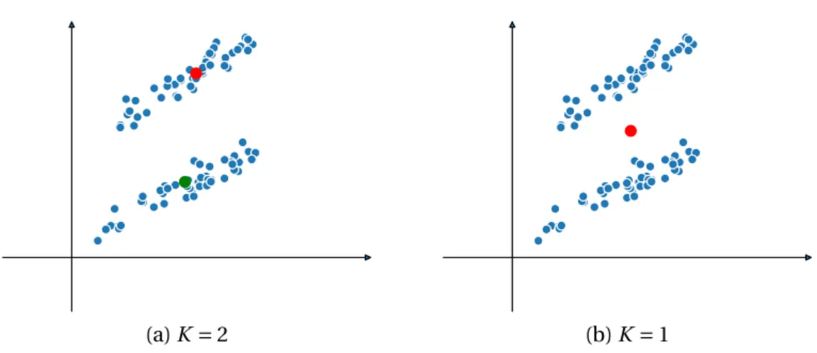
2.12 PCA in 2D . . . 25

2.13 PCA vs.k-means vs. NMF . . . 26

2.14k-means in 2D . . . 27

2.15 NMF in 2D . . . 29

2.16 RA in 2D . . . 30

3.1 Label randomization test error . . . 34

3.2 Support of a ReLU activation matrix . . . 39

3.2 Image datasets . . . 43

3.3 Layer-by-layer NMF compression . . . 46

3.4 NMF reconstruction error . . . 47

3.5 Detecting memorization via matrix factorization: CIFAR-10 . . . 49

3.6 Detecting memorization via matrix factorization: Various datasets . . . 50

3.7 Detecting memorization with i.i.d. batches . . . 52

(14)

List of Figures

3.9 Detecting generalization via compression . . . 54

3.10 NMF for early stopping . . . 55

3.11 Detecting memorization on VGG-19 . . . 57

3.12 NMF runtime on a typical ImageNet batch . . . 58

4.1 NMF heatmap extraction pipeline . . . 61

4.2 NMF and PCA heatmaps withK=3 with VGG-19 on ImageNet 1 . . . 64

4.6 Incremental NMF with VGG-19 on iCoseg 1 . . . 69

4.7 Incremental NMF with VGG-19 on iCoseg 2 . . . 70

4.8 Incremental NMF with ResNet-50 on iCoseg 1 . . . 72

4.9 Incremental NMF with ResNet-50 on iCoseg 2 . . . 73

4.10 Average IoU score for NMF with different layers of VGG-19 on iCoseg . . . 79

4.11 Example NMF heatmaps with VGG-19 on PASCAL-Part 1 . . . 81

4.12 Example NMF heatmaps with VGG-19 on PASCAL-Part 2 . . . 82

5.1 NMF as a bipartite graph . . . 88

5.2 Gradient ascent visualization of NMF basis derived from VGG-16 on iCoseg 2 . 90 5.3 Gradient ascent visualization of NMF basis derived from VGG-16 on iCoseg 2 . 91 5.4 Gradient ascent visualization of NMF basis derived from ResNet-50 on iCoseg 2 92 5.5 Gradient ascent visualization of NMF basis derived from ResNet-50 on iCoseg 3 93 5.6 Example images from Paris buildings with NMF heatmaps from VGG-16 . . . . 95

5.7 Example images from Paris buildings with NMF heatmaps from ResNet-50 . . . 96

5.8 NMF global image descriptor extraction pipeline . . . 99

5.9 Image retrieval with NMF top 5 . . . 100

(15)

List of Tables

3.1 Neural network architectures . . . 45

4.1 Part co-segmentation with VGG-19 on iCoseg . . . 78

4.2 Object co-segmentation on iCoseg . . . 78

4.3 Co-localization on PASCAL VOC 2007 . . . 83

4.4 Part co-segmentation with VGG-19 on PASCAL-Part . . . 84

4.5 Part co-segmentation comparison against state-of-the-art . . . 85

5.1 Instance-based retrieval mAP with NMF and other methods . . . 101

5.2 NMF IoU scores on Oxford and Paris Buildings query sets . . . 103

(16)

(17)

Abbreviations and Notation

List of Abbreviations

Abbreviation Description

NN Artificial neural network CNN Convolutional neural network SGD Stochastic gradient descent PCA Principal component analysis NMF Non-negative matrix factorization

RA Random ablations

ReLU Rectified-linear unit BN Batch normalization

(18)

List of Tables

List of Symbols

Symbol Description

R+ Non-negative real numbers [0, inf)

M,P arbitrary integers representing high dimensional spaces, e.g.RM₊

Λ(·) A function representing a neural network

Λi(·) A function representing theith layer of a neural network

` A loss function defining an optimization objective, not to be confised with `2 The Eculidean norm

X,X,x Neural network input in tensor, matrix and vector form, respectively

I An input image

A,A,a Neural network activations in tensor, matrix and vector form, respectively ˆ

A, ˆA, ˆa Approximation of activations via matrix factorization

X,Z Random variables representing NN input and hidden activation respectively ˆ

y NN last layer output

y Ground truth target NN should predict

Y A random variable distributed over ground truth targets

X×Y The true data distribution of input output pairs

A,B Generic random variables

P,_I,_C,_H The probability operator, mutual information, common information, and Shan-non entropy

V A matrix holding basis vectors of a matrix factorization

U A matrix holding per-sample coefficients for matrix factorization

N Number of samples in a dataset or batch

H Height of image or feature map

W Width of image or feature map

C Number of channels at a convolutional layer

K Positive integer rank of matrix factorization, or a random variable defining a categorical distribution on matrix factors

T Number of output classes

c,k,t A specific channel, factor, or target, i.e., 1≤c≤C, 1≤k≤K, 1≤t≤T

F A random variable defining a categorical distribution over each of theKmatrix factors

a,b,i,j Genetic subscripts for enumerating collections D,_Dtest Datasets used for training and testing, respectively

i A discrete random variable indexing a batch or dataset withP(i=i)=_N1

p The probability of randomizing a training label supp Thesupportof a matrix

(19)

List of Tables Symbol Description

U The matrixUreshaped and rescaled to form a tensor of heatmaps B The tensorUafter binarization

G A tensor containing ground truth binary segmentation masks. Unlikey, this is not used for NN training.

R Number of relevant images with respect to a query image

r The number of relevant images retrieved up to a given rank

(20)

(21)

1

Introduction

S

ince the advent of digital computers in the 1940s, researchers have sought to use them to automate tasks traditionally solved by human labor. As computational resources grew, so did the desire to automate more complex and high-level tasks, such as translating natural language texts, recognizing objects in images, etc.

Early strides towards that goal were based on rigid rule-based systems, distilling expert knowl-edge of a task-specific domain. These systems, however, did not scale to the level ofvariation

which exists in most real-world inputs. A task as simple as, for instance, recognizingdog

images requires approximating a function which maps thousands or even millions of pixels into a yes/no decision, while considering that dogs can be large or small, light or dark, 4-legged or 3-legged, indoors or outdoors - but are not to be confused with cats or even wolves. For such problems,machine learningproposed to design algorithms that automaticallylearnhow to solve a given task.

For example, the most common paradigm in machine learning issupervised learning, i.e., learning by example. In this setting, a dataset is given which consists of input-output pairs, and a parametric model is trained (i.e., its parameters are gradually refined) to predict the output given the input.

The availability of large datasets and powerful computational resources over the past decade has facilitated the rise in popularity ofdeep neural networks. This flexible class of models is at once general, i.e., requiring little domain-specific expertise, while nonetheless showing state-of-the-art performance across diverse domains. This technology has had a profound impact on the high-tech industry, with thedeep learningmarket expected to reach $US 18 Billion by 20241.

(22)

Chapter 1. Introduction T rai n set a ccur a cy 6 Epochs (a) Training curves

T est set a ccur a cy 7 Epochs (b) Test curves

Figure 1.1 – Shown here are (a) training and (b) test curves during training of six convolu-tional neural networks on the CIFAR-10 dataset forced into different degrees of memorization. Marked in red is the outcome at the end of the training procedure.Given the final training set accuracy, is it possible to predict the test set accuracy?In this thesis we find that a distinguishing property which characterizes the difference between these networks, and correlates with better generalization and less memorization, is thenon-negative rankof their activation matrices. However, the success of deep networks has also been accompanied by a certain measure of obfuscation. The factors determining the success or failure of learning are not well understood, and methods of evaluating what was learned are limited.

For instance, while the ultimate goal is togeneralizewell to new data, which is not seen during training, some models are prone tooverfitting, i.e., simply memorizing the training data. In spite of having millions and even billions of parameters, deep neural networks have shown a measure of resilience to this phenomenon, defying the traditional “wisdom” that models with many parameters are likely to overfit. The factors governing a network’s tendency to overfit are still subject to intensive study these days.

Consider for instance the learning curves in Figure 1.1. Although all networks achieve perfect accuracy on their training sets, they have very different levels of generalization. What is the distinguishing factor between these networks? Can it be detected independently of a test set?

(23)

1.1. Thesis contributions and outline In this thesis we propose thatcompressionis a key factor, distinguishing between networks that generalize well and those that simplymemorizetheir training data. Any predictive rule with a degree of generalitymustignore certain aspects of the instance to which it is applied, effectively compressing it by discarding irrelevant information.

The notion that compression is a hallmark of well-generalizing models is not new. It is an extension of a principle going back to antiquity and made famous as Occam’s razor: “Entities are not to be multiplied beyond necessity”. In this case, we prefer a network that learns one general rule that accommodates many inputs, over a network that learns many specific rules that accommodate individual inputs.

Compression not only gives us a criterion by which to evaluate generalization behavior, it also addresses questions regarding theinterpretationof neural networks. It is natural to askwhya certain prediction was made, by which reasoning, or by considering which aspects of the input. The nonlinear interactions between the millions of parameters makes exact answers to these questions incomprehensible to human beings. As these networks are deployed into products and services all around us - from targeted advertisement on social media to autonomous vehicles - there is a growing need to validate and understand the outcome of learning. By examining the compression a convolutional neural network applies to images, we can createheatmapswhich allow us to see how a deep neural network conceptualizes its input. In Figure 1.2 we show an example of this visualization, showing that in a deep network layer, a scene or object is decomposed into its constituent parts. This demonstrates how the network discards information it finds irrelevant, such as scale, perspective, various object deformations etc. At the same time, for the object recognition task it was trained to accomplish, the presence or absence of specific entities, e.g.,towerorperson, are deemed important enough to retain. Furthermore, by characterizing images using the information a convolutional neural network considers relevant about them, we cansemanticallycompare two images. This gives a mecha-nism with which tosearchfor semantically similar images given a query image, andlocalize

the semantically matching regions within the images.

1.1 Thesis contributions and outline

Our main contribution is actualizing the idea of using compression into a working algorithm. Our tool of choice isnon-negative matrix factorization(NMF) [59], which is applicable to neural network layers with non-negative activation, e.g. by using the popularrectified-linear

activation function (section 2.2.2). Let A∈RP+×M be an intermediate representation

(24)

Chapter 1. Introduction

(a) Pyramids,K=4

(b) Taj Mahal,K=3

Figure 1.2 –What in this picture is the same as in the other pictures? Non-negative matrix factorization allows us to see how a deep CNN trained for image classification would answer this question. Here shown is an example of VGG-19 trained on ImageNet classification, and then applied to subsets from the iCoseg dataset. (a) Pyramids, animals and people correspond across images. (b) Monument parts match with each other.

representation into two parts:

A≈U V (1.1)

whereU∈RP+×K,V ∈RK+×M. WhenK is the smallest integer which maintainsA=U V, it is

(25)

1.1. Thesis contributions and outline

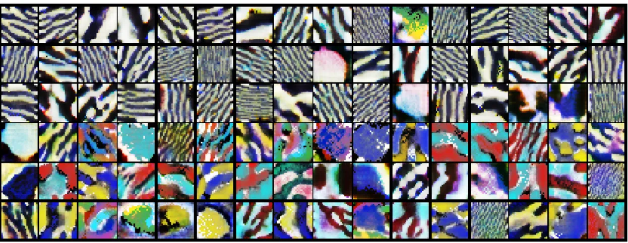
(a) Pyramids,K=4

(b) Taj Mahal,K=3

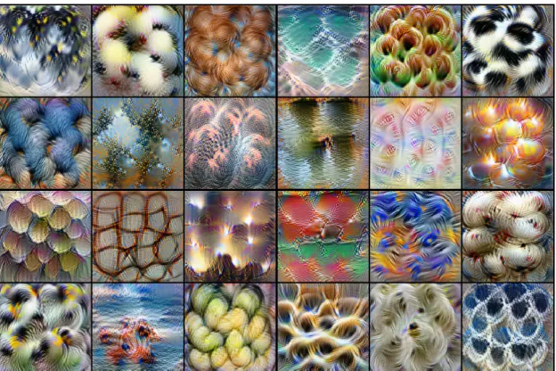
Figure 1.3 – Gradient ascent visualization of the features obtained through non-negative matrix factorization applied to VGG-19 activation for thePyramidsandTaj Mahalsubsets from iCoseg. These visualizations of the rows ofV correspond to the heatmap visualizations of the columns ofUshown in Figure 1.2 using the same color encoding, i.e., the blue framed visualizations above correspond to the blue heatmaps in each corresponding row.

In Chapter 2 introduce interesting properties of NMF as well other factorization methods. In the same chapter we review deep neural networks, and convolutional networks in particular, with a focus on the challenges posed by generalization and interpretation.

In Chapter 3 we derive an upper bound over the amount of memorization in a network layer, expressed in terms of the non-negative rank of its activation matrices. We then explicitly apply compression to the intermediate representations learned by deep neural networks, which allows us to compare neural networks and determine which one is likely to generalize better -without the use of a validation set.

We show empirically that NMF is more effective than other matrix factorization techniques at distinguishing between memorization and generalization. Our method is also effective during training, which we demonstrate by performingearly stopping, before overfitting commences. Matrix factorization methods have been used for exploratory data analysis for decades. As a dimensionality reduction method, matrix factorization retrieves a compressed representation of the data, with fewer redundancies and correlations. When the dimensionality is sufficiently reduced, qualitative interpretation by human beings is made possible.

(26)

Chapter 1. Introduction

We show that this decomposition distills much of the semantics learned by a deep convolu-tional neural network. We roughly characterizeUas “where” andV “what”.

In Chapter 4, we use theUmatrix of the NMF decomposition to produce heatmaps as in Figure 1.2, which offer an interpretable view into what information the network considers relevant and what information it discards. We find that for object recognition, the network learns to recognize fine-grained objectparts, with invariance to complex transformations and noise. For instance, for the task of detectingcarswe see that color is not a discriminative feature, whereas the presence or absence ofwheelsis.

We quantitatively demonstrate the rich semantics encoded in the matrix factors by applying them to real-world tasks such as co-localization and co-segmentation of a common object across a set of images. We obtain state-of-the-art results, with performance comparable or surpassing even hand-crafted domain-specific methods.

Each heatmap produced by the matrixU corresponds to a network feature which is stored in matrixV. For instance, using feature visualization techniques can visualizeV as shown in Figure 1.3. These visualization are informed of the original images shown in Figure 1.2 only through the features inV.

In Chapter 5 we use the matrixV to describe an image globally as abag-of-concepts. We evaluate this representation by performingimage search. Specifically, we derive global image descriptors usingV and show they can be used to retrieve images containing similar objects, with all the invariances learned by the network. For example, given an image of adog, we search through a dataset and rank highly other images that portraydogs, regardless of scale, rotation and evendog breed.

By combining information from bothUandV we performinstance-basedsearch, i.e., given an image of a building, we rank highly only images of that particular building, and not images of other similar looking buildings. We again find that this approach outperforms comparable state-of-the-art methods.

In Chapter 6 we conclude the thesis with a summary of our contributions and directions for future work.

(27)

2

Related Work

2.1 Introduction

The methods proposed in this thesis concern various aspects of neural networks in general, and convolutional neural networks in particular. The first half of Section 2.2 therefore provides an introduction to neural networks, focusing on the necessity for multiple layers in order to achieve good performance on complex prediction tasks, and describing common design choices in modern networks.

Section 2.2 then proceeds with an introduction of the two main themes of our work. We discuss empirical methods to detectoverfitting, its impact on generalization, and theoretical work providing upper bounds on thegeneralization error. We then introduce the challenge of

network interpretability, reviewing existing approaches with a focus on convolutional neural networks.

Our tool of choice for both detecting memorization and opening an interpretable window into convolutional neural networks, isnon-negative matrix factorization. We introduce this method as well as other matrix factorization methods in Section 2.3.

2.2 Convolutional neural networks

2.2.1 From single neurons to deep convolutional neural networks

The class of computational models referred to asartificial neural networks(NNs) contains many diverse models. A common characteristic to all NNs, which they share with their biological namesakes, is the composition of simple computational units, the so-called neurons, into a larger collective, capable of computing more complex functions.

(28)

Chapter 2. Related Work y

2

0

2

4

6

8

4.8

5.0

5.2

5.4

5.6

5.8

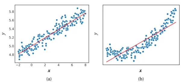
y 2 0 2 4 6 8 4.9 5.0 5.1 5.2 5.3 5.4 5.5 5.6 x x (a) (b)

Figure 2.1 – A single-neuron neural network with identity activation and mean squared error loss is equivalent to linear regression. Model predictions lie on the red line. (a) The data follows a linear distribution and the linear regression gives accurate predictions. (b) The data follows a non-linear distribution and linear-regression is too limited to give accurate predictions.

Linear-prediction: Single neuron and single layer At its simplest, a single neuron is a functionΛ:RM→R:

Λ(x)=f(x>w+b) (2.1)

i.e., a weighted-sum of the input vectorxwith weightsw, both inRM, followed by the addition of a bias termb∈R. Finally theactivation function f is applied to form the neuron output, called simply theactivation.

A single-neuron NN can already retrieve common statistical models. We denote the output prediction of a NN as ˆy=Λ(x). LettingD={xi,yi|1≤i≤N} be a training dataset of input-output samples, the weightsw and the bias termb are trained to minimize the empirical loss: `D= 1 N X x,y∈D `( ˆy,y) (2.2) w∗,b∗=arg min w,b `D (2.3)

where`is thelossfunction, measuring the prediction error.

Different settings of activation and loss functions define different models. For instance, as shown in Figure 2.1, wheny∈R,linear regressioncan be cast as a single-neuron NN with

(29)

2.2. Convolutional neural networks

identityactivation and squared-error loss:

f(a)=a (2.4)

`( ˆy,y)= kyˆ−yk22 →( ˆy−y)2ify∈R

Similarly, for binary classification withy∈{0, 1}, as in Figure 2.2, setting the activation function to thelogistic functionand loss tobinary cross-entropyresults in a single-neuron NN which performs logistic regression:

f(a)= 1

1+e−a (2.5)

`( ˆy,y)= −ylog( ˆy)−(1−y) log(1−yˆ)

An example of multiple neurons composed together arises with the generalization of logistic regression to the case wherey∈{1,· · ·,T} and we wish to classifyxas belonging to exactly one ofT classes. This is accomplished by consideringT neurons jointly, where we define the

jth neuron output as the score or probability of belonging to thejth class. In this case, the weight vectors of the individual neurons are stacked into a single weight matrix,W ∈RM×T, and similarly all bias terms to a vector,b∈RT. Computing the NN output prediction proceeds as before:

ˆ

y=Λ(x)=f(x>W+b) (2.6)

A suitable activation function in this case is thesoftmaxfunctionf(x)=_k_eexx_k

1, which

normal-izes its input to form a probability distribution. The cross-entropy loss in this case reduces to the negative log-likelihood of the correct class`( ˆy,y)= −log ˆyy. This model is referred to as softmax regression.

Neurons combined as in Eq. (2.6) are said to form alayerof widthT. A layer parameterized this way is called “fully-connected”, since every input affects every output. A fully-connected layer withMinputs andT outputs has a total (M+1)·T trainable parameters.

An important property of the single-layer models described thus far is that they makelinear

predictions. This can be seen in Figures 2.1 and 2.2. Linear regression explicitly parameterizes a line equation on which its predictions lie, and both logistic and softmax regression are characterized by linear decision boundaries.

For classification, the linearity of decision boundaries does not pose a limitation if, indeed, the vectors associated with a labela, i.e.,Xa={xi|yi=a}, arelinearly separablefrom the vectors

(30)

Chapter 2. Related Work x1 1.0 0.5 0.0 0.5 1.0 1.0 0.5 0.0 0.5 1.0 x 2 1 0.0 0.2 0.4 0.6 0.8 1.0 1.2 0.0 0.2 0.4 0.6 0.8 1.0 1.2 x2 x₂2 (a) (b)

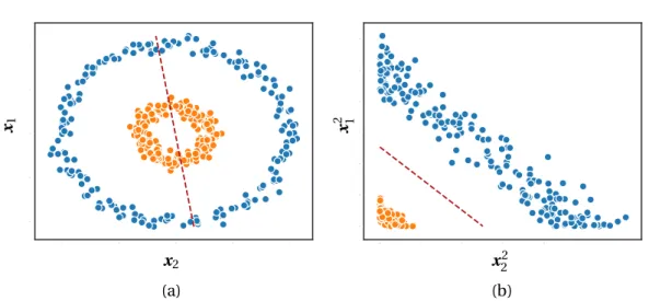
Figure 2.2 – A single-neuron neural network with logistic activation and binary cross-entropy loss is equivalent to logistic regression. The decision boundary at ˆy=0.5 is shown in red. (a) Logistic regression cannot separate clusters which are not linearly-separable. (b) An appropriate transformation can extract features that result in linear-separability.

minimize the loss.

However, ifXa isnotlinearly-separable fromXb, as in Figure 2.2a, inherent model error is introduced that cannot be overcome by any setting of the parametersW andb.

Feature extraction: multiple layers

To overcome this issue, the input vectorsxmust first be transformed, by an additional function

Λh, into having linearly-separable structure. The transformed output, calledfeatures, can then be fed to the single-layer classifier:

ˆ

y=Λ(Λh(x)) (2.7)

In the case shown in Figure 2.2a, although the data is given as two dimensional vectors

x=<x1,x2>, the cluster identity is determined by the radius lengthx₁2+x₂2. SettingΛh(x)=<

x₁2,x2₂>is therefore an adequate transformation, which yields the linearly-separable clusters shown in Figure 2.2b.

The question remains, however, how to find appropriate features without requiring case-by-case analysis. Such analysis typically involves considerable investment and is limited by the level of domain-specific expertise available to the feature designer.

(31)

2.2. Convolutional neural networks One solution is to augment the input with higher-order interactions, e.g., the squared inputs used in the above example. It is unclear, however, how complex these interactions must be in order to achieve linear separability. Furthermore, adding all interaction terms of a certain order increases the input size combinatorially, which quickly makes the weight matrixW large. Over-parameterized layers have higher space and time complexity, and are exposed to the danger ofoverfitting, discussed in section 2.2.3.

A different approach is to model the functionΛhsimilarly to the functionΛ:

Λh(x)=g(W_h>x+bh) (2.8)

wheregis an activation function andWh∈RM×P. We accordingly redefineW∈RP×T. The model prediction now becomes a composition:

ˆ

y=Λ(Λh(x)) (2.9)

and the parameters ofΛhandΛare both subject to training. Analyzing the features extracted byΛhis an interesting challenge, as discussed in Section 2.2.4.

In the resultingtwo-layermodel,Λis called theoutput layerandΛhis referred to as ahidden

layer, since itsP-dimensional output activation is a latent code without any a-priori assigned meaning. The terminput layeris sometimes used to refer to the inputxitself. This layered architecture is calledfeed-forward, since obtaining the prediction involves feeding the output of each layer forward to the next layer.

The layerΛhhas limited expressive power, since it consists of only a single linear transfor-mation followed by an element-wise activation function. Achieving linear-separability may require more complex transformations. In this case, complexity could be increased by intro-ducing additional layers to the model, increasing itsdepth.

We thus arrive to the generalL-layer feed-forward NN model, which is the underlying paradigm for most modern NN architectures today:

a0=x (2.10)

ai=Λi(ai−1), 1≤i≤L

ˆ

y=aL

The number of hidden layers,L−1, their widths, and the activation functions used are hyper-parameters defining the NN architecture, and are set by the network designer.

(32)

Chapter 2. Related Work

The vectoraiis the activation vector at layeri, also referred to as thefeaturesextracted by the firstilayers. The activation of the final layer is the output prediction ˆy.

The intuition behinddeep learningsuggests that the deeper the layeri, the more abstract and semantically meaningful are its features [12].

Convolution

Computer vision deals with image data for tasks such as object recognition and segmentation. Using fully-connected NNs to solve these tasks quickly runs into a scalability issue: image data can have hundreds-of-thousands or millions of dimensions, even at moderate image resolutions.

To resolve this, theconvolutionalneural network (CNN) was introduced [58]. In this net-work the basic layer computation is changed to have two properties: local-connectivity and translation-invariance. These properties drastically reduce the number of network parameters, thereby reducing computational load and the danger of overfitting.

Local-connectivity means that by applying small filters to image patches, only interactions between near-by pixels are considered. This is based on the assumption that, for instance, a pixel near the top-left corner of the image and a pixel near the bottom-right corner, are unlikely to be related in a consistent manner which can be useful for making predictions. Translation-invariance means we can use the same local filter in all spatial positions. This is based on the assumption that image statistics distribute identically across the spatial dimen-sions of the image.

With the properties combined, the result is that a CNN layer performs a 2D spatial-convolution (or cross-correlation) between the input image and a set of learned filters. Note that the same local-connectivity and translation-invariance assumptions can be applied to any directional data, e.g., time-series or text data, in which case convolution and filters are 1D.

Formally, an image is represented as a tensorI∈RCI×HI×WI_{, where}_H

IandWIare the height

and width of the image respectively, andCIis the number of channels, e.g.,CI=3 for RGB

color images.

The weight tensor of a convolutional layerW∈RCout×Cin×HW×WW _{is viewed as a set of}_C

out

filters, each of spatial dimensionsHW×WWand as many channels as the layer input. The bias

(33)

2.2. Convolutional neural networks

Figure 2.3 – A schematic of AlexNet. Figure taken from Krizhevsky et al. [55].

A convolutional layer operates in the image’s 2D space and computes: Ai∈RCout×HAi×WAi

Ai=Λi(Ai−1) such that [Λi(Ai−1)]c=f(Ai−1∗Wc+b) (2.11) where∗denotes convolution, andAi−1is the layer input, e.g.Ai−1=I, and thusCin=CAi−1.

Each of theCoutchannels of the resulting activation tensor,Λ(X), is also called afeature map,

since it is a 2D activation map where each value represents a feature response with respect to an image patch.

The output dimensionsHAi×WAi, being a function ofHIandWI, vary from image to image.

In general, convolution produces an output with decreased spatial dimension. To account for this, padding is added at each layer to give an output with the same spatial dimensionality as the input.

Commonly, spatial dimensions are reduced with explicit down-sampling, accompanied by an increase in the channel dimension. This further reduces the memory and computation requirements. Down-sampling is accomplished by setting the stride of convolutions orpooling

operations to be greater than one.

A common form of pooling ismax-pooling. Defined by a window of sizeHp×Wp, the pooling window slides over the image akin to the convolution operation, and returns at every position the maximal value within the window. When applied to an activation tensor withCchannels, max-pooling is applied to each channel separately, i.e., given inputA∈RC×Hp×Wp_{, max pooling}

returns aC−d i mensi onal vector, having pooled the spatial dimensions.

Arguably the first successfully trained large-scale CNN is AlexNet [55]. It consist of several convolutional layers, followed by several fully-connected layers. A schematic of AlexNet is shown in Figure 2.3.

(34)

Chapter 2. Related Work

Figure 2.4 – A schematic of VGG16. VGG networks follow the design of AlexNet, but are deeper and exclusively use small filters. Figure taken from blog.heuritech.com.

Trained on ImageNet [80], AlexNet classifies images as belonging to one of 1K classes. With a total of 60M parameters, this network achieved a top-1 accuracy of 62.5% and top-5 accuracy of 83%.

The networks VGG-16 and VGG-19 [87] closely follow the architecture of AlexNet. However, they exclusively use small 3×3 convolutional filters (compared to 11×11 in the first layer of AlexNet), and have increased depth. VGG-16 improved CNN performance on ImageNet to classification to top-1 accuracy of 74.4% and top-5 accuracy of 91.9%. See Figure 2.4 for a schematic.

2.2.2 Training and gradient flow

Gradient optimization

Minimizing the objective function of the logistic regression model of Eq. (2.4) can be done analytically: computing the gradient of the loss with respect towand setting it to zero gives the well-knownnormal equation, which has a closed-form solution yielding the optimalw. Logistic regression, in Eq. (2.5), on the other hand, does not lend itself to a closed-form solution. Instead, its parameters are iteratively updated withgradient descent(GD). Starting from a random parameter initialization, at every iteration the gradient∇w`is computed, and

(35)

2.2. Convolutional neural networks

317

Xavier Glorot, Antoine Bordes, Yoshua Bengio

Figure 1: Left:Common neural activation function motivated by biological data.Right: Commonly

used activation functionsin neural networks literature: logistic sigmoid and hyperbolic tangent (tanh).

hyperbolic tangent(see Figure 1, right), which are

equivalent up to a linear transformation. The hy-perbolic tangent has a steady state at 0, and is therefore preferred from the optimization

stand-point (LeCun et al., 1998; Bengio and Glorot,

2010), but it forces an antisymmetry around 0 which is absent in biological neurons.

2.2 Advantages of Sparsity

Sparsity has become a concept of interest, not only in computational neuroscience and machine learning but also in statistics and signal processing (Candes and Tao, 2005). It was first introduced in computational neuroscience in the context of sparse coding in the vi-sual system (Olshausen and Field, 1997). It has been a key element of deep convolutional networks exploit-ing a variant of auto-encoders (Ranzatoet al., 2007,

2008; Mairal et al., 2009) with a sparse distributed

representation, and has also become a key ingredient in Deep Belief Networks (Leeet al., 2008). A sparsity penalty has been used in several computational neuro-science (Olshausen and Field, 1997; Doiet al., 2006) and machine learning models (Leeet al., 2007; Mairal

et al., 2009), in particular for deep architectures (Lee

et al., 2008; Ranzatoet al., 2007, 2008). However, in

the latter, the neurons end up taking small but non-zero activation or firing probability. We show here that using a rectifying non-linearity gives rise to real zeros of activations and thus truly sparse representations. From a computational point of view, such representa-tions are appealing for the following reasons:

• Information disentangling. One of the

claimed objectives of deep learning

algo-rithms (Bengio, 2009) is to disentangle the factors explaining the variations in the data. A dense representation is highly entangled because almost any change in the input modifies most of

the entries in the representation vector. Instead, if a representation is both sparse and robust to small input changes, the set of non-zero features is almost always roughly conserved by small changes of the input.

• Efficient variable-size representation. Dif-ferent inputs may contain di↵erent amounts of in-formation and would be more conveniently repre-sented using a variable-size data-structure, which is common in computer representations of

infor-mation. Varying the number of active neurons

allows a model to control the e↵ective dimension-ality of the representation for a given input and

the required precision.

• Linear separability. Sparse representations are also more likely to be linearly separable, or more easily separable with less non-linear machinery, simply because the information is represented in a high-dimensional space. Besides, this can reflect the original data format. In text-related applica-tions for instance, the original raw data is already very sparse (see Section 4.2).

• Distributed but sparse. Dense distributed rep-resentations are the richest reprep-resentations, be-ing potentially exponentially more efficient than purely local ones (Bengio, 2009). Sparse repre-sentations’ efficiency is still exponentially greater, with the power of the exponent being the number of non-zero features. They may represent a good trade-o↵ with respect to the above criteria. Nevertheless, forcing too much sparsity may hurt pre-dictive performance for an equal number of neurons, because it reduces the e↵ective capacity of the model.

(a) Sigmoid activation functions

318

Deep Sparse Rectifier Neural Networks

Figure 2: Left: Sparse propagation of activations and gradients in a network of rectifier units. The

input selects a subset of active neurons and computation is linear in this subset. Right: Rectifier and softplus activation functions.The second one is a smooth version of the first.

3 Deep Rectifier Networks 3.1 Rectifier Neurons

The neuroscience literature (Bush and Sejnowski,

1995; Douglas and al., 2003) indicates that

corti-cal neurons are rarely in their maximum saturation

regime, and suggests that their activation function can

be approximated by a rectifier. Most previous stud-ies of neural networks involving a rectifying activation function concern recurrent networks (Salinas and Ab-bott, 1996; Hahnloser, 1998).

The rectifier function rectifier(x) = max(0, x) is one-sided and therefore does not enforce a sign symmetry1

or antisymmetry1_{: instead, the response to the}

oppo-site of an excitatory input pattern is 0 (no response). However, we can obtain symmetry or antisymmetry by combining two rectifier units sharing parameters.

Advantages The rectifier activation function allows a network to easily obtain sparse representations. For example, after uniform initialization of the weights, around 50% of hidden units continuous output val-ues are real zeros, and this fraction can easily increase with sparsity-inducing regularization. Apart from be-ing more biologically plausible, sparsity also leads to mathematical advantages (see previous section). As illustrated in Figure 2 (left), the only non-linearity in the network comes from the path selection associ-ated with individual neurons being active or not. For a given inputonly a subset of neurons are active. Com-putation islinearon this subset: once this subset of neurons is selected, the output is a linear function of

1_{The hyperbolic tangent absolute value non-linearity}

|tanh(x)|used by Jarrettet al.(2009) enforces sign symme-try. A tanh(x) non-linearity enforces sign antisymmetry.

the input (although a large enough change can trigger a discrete change of the active set of neurons). The function computed by each neuron or by the network output in terms of the network input is thus linear by

parts. We can see the model as anexponential

num-ber of linear models that share parameters (Nair and

Hinton, 2010). Because of this linearity, gradients flow well on the active paths of neurons (there is no gra-dient vanishing e↵ect due to activation non-linearities of sigmoid or tanh units), and mathematical investi-gation is easier. Computations are also cheaper: there is no need for computing the exponential function in activations, and sparsity can be exploited.

Potential Problems One may hypothesize that the hard saturation at 0 may hurt optimization by block-ing gradient back-propagation. To evaluate the poten-tial impact of this e↵ect we also investigate the soft-plus activation:softplus(x) =log(1+ex_{) (Dugas}_{et al.}_,

2001), a smooth version of the rectifying non-linearity. We lose the exact sparsity, but may hope to gain eas-ier training. However, experimental results (see Sec-tion 4.1) tend to contradict that hypothesis, suggesting that hard zeros can actually help supervised training. We hypothesize that the hard non-linearities do not

hurtso long as the gradient can propagate along some

paths, i.e., that some of the hidden units in each layer

are non-zero. With the credit and blame assigned to

these ON unitsrather than distributed more evenly, we

hypothesize that optimization is easier. Another prob-lem could arise due to the unbounded behavior of the activations; one may thus want to use a regularizer to prevent potential numerical problems. Therefore, we use theL1penalty on the activation values, which also

promotes additional sparsity. Also recall that, in or-der to efficiently represent symmetric/antisymmetric behavior in the data, a rectifier network would need

(b) Rectified-linear activation function Figure 2.5 – The activation function plays a crucial role in the convergence properties of a deep NN. (a) Saturating activation functions have small gradients far from the origin, which slows down learning as NN weights grow in magnitude. (b) The rectified-linear function [37], on the other hand, has a gradient of 1 for all positive activations. The non-negativity of the rectified-linear function enables us to use NMF in our analysis of CNN activations. Figure taken from Glorot et al. [37].

the weights are updated as:

w←w−α∇w (2.12)

whereαis a hyper-parameter controlling thestep size.

When the step size is not too large, GD is guaranteed to find the globally optimal value ofw, because the single-layer logistic regression model has aconvexobjective function.

A NN or CNN with many layers, however, defines a highly non-convex function. Minimizing such a function with GD could theoretically “get stuck” in a sub-optimal local minimum. With the availability of large datasets for training,stochasticgradient descent (SGD) has been proposed, which performs a gradient update based on a stochastically sampled subset of the data, called a batch. The introduction of sampling noise could account for the good performance of (stochastic) gradient descent methods in practice, since the noise allows the network to escape from narrow local minima [51].

Augmentations of SGD have also been proposed, such as SGD with momentum [74], Adagrad [29] and ADAM [52]. These methods all maintain a per-parameter learning rate, resulting in faster convergence than standard SGD.

One of the main challenges of optimization with SGD variants is the problem ofvanishing and exploding gradients. Specifically, the gradient is computed by back-propagating the error

(36)

Chapter 2. Related Work

8

Ta

b

le

2

.

C

la

ss

ifi

ca

ti

o

n

erro

r

(%

)

o

n

th

e

C

IF

A

R

-1

0

te

st

se

t

u

si

n

g

d

i↵

ere

n

t

a

ct

iv

a

ti

o

n

fu

n

ct

io

n

s.

case

Fig.

Res

Net-110

Res

Net-164

original

Residual

U

nit

[1

]

Fig.

4

(a)

6.61

5.93

BN

af

ter

addition

Fig.

4

(b)

8.17

6.50

ReLU

b

efor

e

addi

ti

on

Fig.

4

(c)

7.84

6.14

ReLU-onl

y

pr

e-acti

v

ati

on

Fig.

4

(d)

6.71

5.91

full

pre-activ

ation

Fig.

4

(e)

6.37

5.46

BN

Re

LU

w

e

ig

ht

BN

w

e

ig

ht

addit

ion

ReLU

x

l

x

l+ 1

Re

LU

wei

g

h

t

BN

Re

LU

wei

g

h

t

BN

addit

ion

x

l

x

l+ 1

BN

Re

LU

wei

g

h

t

BN

wei

g

h

t

addit

ion

ReLU

x

l

x

l+ 1

BN

Re

LU

wei

g

h

t

BN

Re

LU

wei

g

h

t

addit

ion

x

l

x

l+ 1

wei

g

h

t

BN

Re

LU

wei

g

h

t

BN

Re

LU

addit

ion

x

l

x

l+ 1

(

a

)

or

i

g

in

a

l

(b)

B

N

a

f

te

r

ad

d

i

t

i

o

n

(c

)

R

e

L

U

b

e

f

o

re

ad

d

i

t

i

o

n

(d)

R

e

L

U

-o

n

l

y

p

r

e

-a

c

tiv

a

tion

(e

)

fu

ll

p

r

e

-ac

tiva

tion

Figur

e

4.

V

a

ri

o

u

s

us

a

g

es

o

f

a

ct

iv

a

ti

o

n

in

T

a

b

le

2

.A

llt

h

es

eu

n

it

s

co

n

si

sto

f

th

es

a

m

e

co

m

p

o

n

en

ts

—

o

n

ly

th

e

o

rd

ers

a

re

d

i↵

ere

n

t.

3.

2

D

is

c

u

ss

ion

s

As

in

d

ic

at

ed

b

y

th

e

gr

ey

ar

ro

w

s

in

F

ig.

2

,

th

e

sh

or

tc

u

t

con

n

ec

ti

on

s

ar

e

th

e

m

os

t

d

ir

ec

t

p

at

h

s

for

th

e

in

for

m

at

ion

to

p

rop

agat

e.

M

u

lt

ip

li

ca

ti

ve

m

an

ip

u

lat

ion

s

(s

cal

in

g,

gat

in

g,

1

⇥

1

con

vol

u

ti

on

s,

an

d

rop

ou

t)

on

th

e

sh

or

tc

u

ts

can

h

am

p

er

in

for

m

at

ion

p

rop

agat

ion

an

d

le

ad

to

op

ti

m

iz

at

ion

p

rob

le

m

s.

It

is

n

ot

ew

or

th

y

th

at

th

e

gat

in

g

an

d

1

⇥

1

con

vol

u

ti

on

al

sh

or

tc

u

ts

in

tr

o

d

u

ce

m

or

e

p

ar

am

et

er

s,

an

d

sh

ou

ld

h

av

e

st

ron

ge

r

rep

res

en

ta

ti

o

n

a

l

ab

il

it

ie

s

th

an

id

en

-ti

ty

sh

or

tc

u

ts

.

In

fac

t,

th

e

sh

or

tc

u

t-on

ly

gat

in

g

an

d

1

⇥

1

con

vol

u

ti

on

co

ve

r

th

e

sol

u

ti

on

sp

ac

e

of

id

en

ti

ty

sh

or

tc

u

ts

(

i.

e.

,

th

ey

cou

ld

b

e

op

ti

m

iz

ed

as

id

en

ti

ty

sh

or

tc

u

ts

).

Ho

w

ev

er

,

th

ei

r

tr

ai

n

in

g

er

ror

is

h

igh

er

th

an

th

at

of

id

en

ti

ty

sh

or

t-cu

ts

,

in

d

ic

at

in

g

th

at

th

e

d

egr

ad

at

ion

of

th

es

e

m

o

d

el

s

is

cau

se

d

b

y

op

ti

m

iz

at

ion

is

su

es

,

in

st

ead

of

re

p

re

se

n

tat

ion

al

ab

il

it

ie

s.

4

O

n

the

U

sa

g

e

o

f

A

ct

iv

a

ti

o

n

F

unct

io

ns

E

x

p

er

im

en

ts

in

th

e

ab

ov

e

se

ct

ion

su

p

or

t

th

e

an

al

y

si

s

in

E

q

n

.(

5)

an

d

E

q

n

.(

8

),

b

ot

h

b

ei

n

g

d

er

iv

ed

u

n

d

er

th

e

as

su

m

p

ti

on

th

at

th

e

af

te

r-ad

d

it

ion

ac

ti

vat

ion

f

Figure 2.6 – Residual connections form the basis of ResNets. In this diagramweightrefers to a linear transformation, BN to batch-normalization,and ReLU is the rectified-linear function. Figure taken from He et al. [44].

[79] from the output layer, through deep layers, into early layers. Through multiplicative interactions along the way, the gradient signal for early layers can have a very small or very large magnitude, leading to slow convergence. The next two sections deal with proposed solutions to this phenomenon.

Activation functions and residual connections

The activation function produces the final layer output and can greatly affect gradient flow. For many years, sigmoidal (“S”-shaped) functions, such as the logistic function and the hyperbolic tangent were widely used, shown in Figure 2.5.

With the advent of deep networks, it was soon realized that sigmoid functions caused gradients to vanish. As network weights grew with every SGD update, activations would be pushed into the high- and low-end plateaus of the sigmoid activation function, where the gradient is very small.

A solution was proposed in the form of rectified-linear units (ReLU) [37]. This activation function, f(x)=max(x, 0), has a gradient that is either 0 or 1, as shown in Figure 2.5b. This allows gradients to flow freely (or not at all), and is now standard in most modern CNNs. ReLU additionally has the property of producing non-negative activations, which enables our analysis of CNN activations using non-negative matrix factorization.

While ReLUs can pass the gradient unaltered, a long chain of linear transformations is still sufficient to hurt network performance. A solution to this issue comes in the form ofresidual connections[44], which tweaks the standard feed-forward pipeline as follows:

(37)

2.2. Convolutional neural networks In other words, the layerΛicomputes aresidualterm, which, once added to the layer input, achieves the desired transformation. Figure 2.6 shows the basic residual block.

This simple change means that the gradient can flow intoai−1throughΛias well asdirectly. The popular ResNet-50, which consists of 50 residual layers, further improves upon the stan-dard feed-forward nets described above, achieving ImageNet classification top-1 accuracy of 79.26% and top-5 accuracy of 94.75%. In addition to residual connections, ResNets employ ReLU activations andbach-normalization, described below.

Initialization and batch-normalization

The random initialization at the start of training has been found to have a significant impact on convergence [64]. Effective initialization methods have been proposed to ensure that the gradient magnitude is maintained constant as it flows from layer to layer [36; 43], improving convergence. These methods, however, only affect SGD iterations near the start of training. Batch-normalization [46], on the other hand, is a method that explicitly normalizes network activations according to the statistics of the current SGD batch, all throughout training. By doing so, the magnitude of the gradients is also controlled, and convergence is accelerated. This technique also is widely incorporated into most modern CNNs, and is applied between the convolution and ReLU activation.

2.2.3 Generalization and overfitting

The training setD={xi,yi|1≤i≤N}∼{X×Y} is a collection ofN samples, each sampled from thedata distribution X×Y over pairs (x,y). In the discussion so far we have referred to NN training as the task of minimizing the empirical loss, ortrainingloss, evaluated usingD, as in Eq. (2.2).

The ultimate goal of learning, however, is to do well on new data, unseen during training. We want to minimize thegeneralization loss:

`X×Y =Ex,y∼X×Y[`(Λ(x),y)] (2.14) The generalization loss is approximated by measuring thetest lossusing a test setDtest, which

contains additional samples fromX×Y not used during training.

Large NNs have the capacity tooverfittheir training set, i.e.,memorizeindividual input-to-output mappings, which does not promote good generalization to new data samples. In this way, the training loss can be minimized while the test loss remains high. This phenomenon is demonstrated in Figure 2.7.

(38)

Chapter 2. Related Work

220 7. Model Assessment and Selection

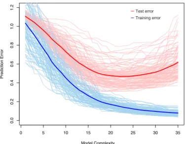
0 5 10 15 20 25 30 35 0.0 0.2 0.4 0.6 0.8 1.0 1.2 Model Complexity Prediction Error

FIGURE 7.1.Behavior of test sample and training sample error as the model

complexity is varied. The light blue curves show the training errorerr, while the

light red curves show the conditional test errorErrT for100training sets of size

50each, as the model complexity is increased. The solid curves show the expected

test errorErrand the expected training errorE[err].

Test error, also referred to as generalization error, is the prediction error

over an independent test sample

Err_T = E[L(Y,fˆ(X))|T] (7.2) where both X and Y are drawn randomly from their joint distribution (population). Here the training setT is fixed, and test error refers to the error for this specific training set. A related quantity is the expected pre-diction error (or expected test error)

Err = E[L(Y,fˆ(X))] = E[Err_T]. (7.3) Note that this expectation averages over everything that is random, includ-ing the randomness in the traininclud-ing set that produced ˆf.

Figure 7.1 shows the prediction error (light red curves) Err_T for 100 simulated training sets each of size 50. The lasso (Section 3.4.2) was used to produce the sequence of fits. The solid red curve is the average, and hence an estimate of Err.

Estimation of Err_T will be our goal, although we will see that Err is more amenable to statistical analysis, and most methods eﬀectively esti-mate the expected error. It does not seem possible to estiesti-mate conditional

–Test error

–Training error

Figure 2.7 – Overfitting is characterized by low training error but high test error. This is due to a model having sufficient capacity to memorize individual input-to-output mappings, at the ex