Wage adjustment and productivity shocks

Uppsala Center for Labor Studies

Department of Economics

Working Paper 2011:14

Wage adjustment and productivity

shocks

Mikael Carlsson, Julián Messina and Oskar

Nordström Skans

Uppsala Center for Labor Studies

Working paper 2011:14

Department of Economics

December 2011

Uppsala University

P.O. Box 513

SE-751 20 Uppsala

Sweden

Fax: +46 18 471 14 78

W

m

c

, j

m

o

n

s

Wage adjustment and productivity shocks

∗

Mikael Carlsson

, Julián Messina

and Oskar Nordström Skans

May 11, 2011

Abstract

We study how workers’ wages respond to TFP-driven innovations in firms’ labor productivity. Using unique data with highly reliable firm-level output prices and quantities in the manufacturing sector in Sweden, we are able to derive measures of physical (as opposed to revenue) TFP to instrument labor productivity in the wage equations. We find that the reaction of wages to sectoral labor productivity is almost three times larger than the response to pure idiosyncratic (firm-level) shocks, a result which crucially hinges on the use of physical TFP as an instrument. These results are all robust to a number of empirical specifications, including models accounting for selection on both the demand and supply side through worker-firm (match)fixed effects. Further results suggest that technological progress at thefirm level has negligible effects on thefirm-level composition of employees.

∗_{We thank John Abowd, Per-Anders Edin, Peter Fredriksson, John Haltiwanger, Marcel Jansen,}

Francis Kramarz, Rafael Lalive, Nuria Rodríguez-Planas and seminar participants at SciencePo, the Helsinki Center of Economic Research (HECER), the Euro-System WDN network, the 6th ECB/CEPR Labor Market Workshop, IFAU, the “Labor Market and the Macroeconomy” confer-ence at Sveriges Riksbank, the LMDG workshop on “Matched Employer-Employee Data: Devel-opments since AKM”, the UCLS Industrial Relations workshop, and the 2010 EEA, EALE/SOLE and LACEA meetings for useful comments. The views expressed in this paper are solely the re-sponsibility of the authors and should not be interpreted as reflecting the views of the Executive Board of Sveriges Riksbank or the World Bank.

†_{Research Department, Sveriges Riksbank E-mail: [email protected].}

‡_{Office of the Chief Economist for Latin America and the Caribbean, World Bank. E-mail:}

[email protected]

§_{Institute for Labour Market Policy Evaluation (IFAU), UCLS, and IZA. E-mail:}

1

Introduction

There is a long-standing debate on the importance of firm-level productivity for individual wages. Building on the extensive literature that followed the work by Abowd, Kramarz, and Margolis (1999), it is by now an established fact that some firms consistently pay higher wages than others, even to identical workers. Yet, surprisingly little is known about the deep determinants of the persistent diff er-ences in firms’ pay, and about how these differences evolve when firms’ economic conditions change.1 Mortensen (2003) argued that productivity differences between firms are closely linked to wage dispersion, and the association between measured labor productivity and individual wages is by now also well documented (Lentz and Mortensen (2010)). However, identifying the direction of causality is not straightfor-ward and, as we argue in this paper, standard identification problems are typically exacerbated by a lack of adequate data on the firm side.2

Assessing the causal impact of firm-level productivity on individual workers’ wages poses three key identification challenges. The first is a measurement issue. Sincefirm-level prices rarely are observed, most previous studies measure firm-level output as revenue divided by an industry-level deflator. This implies that output and productivity measures reflect price differences between firms operating in the

1

A large literature has established an empirical association between wages andfirm level profits.

See Nickell and Wadhwani (1990), Blanchflower and Oswald (1996) and Hildreth and Oswald (1997)

for some of the earlier work and Martins (2009), Arai and Heyman (2009) and Card, Devicienti, and Maida (2009) for recent applications. Differences in profits across firms, just like the case of revenue or sales discussed in the paper, are likely to be driven by demand, productivity and factor input shocks.

2

Fox and Smeets (Forthcoming) and Irarrazabal, Moxnes, and Ulltveit-Moe (2009) have recently looked at the reverse of our question of interest: the impact of unobserved human capital charac-teristics on productivity differences acrossfirms within sectors.

same industry. Importantly, firm-level prices tend to be a function of factor prices, including wages (see e.g. Carlsson and Nordström Skans (Forthcoming)). In order to differentiate betweenfirms with high costs (e.g. due to high wages) andfirms with high productivity it is therefore necessary to account for price differences between firms within industries. When assessing the impact of firm productivity on wages, measures of productivity based on firm-level revenues deflated by an industry-level price index will suffer from reversed causality.

The second challenge stems from firms’ optimizing behavior, which generates a relationship between wages and labor productivity that differs from the causal impact of productivity on wages we want to capture. Intuitively, shocks to wages, other factor prices or product demand will alter the scale of production and/or the capital-labor ratio as well as individual wages. A positive association between wages and productivity may arise if labor productivity responds to idiosyncratic firm-level wage shocks. Think about a positive wage shock. Firms’ optimizing behavior suggests a substitution of labor for capital, which should increase labor productivity. Sometimes this relationship may be triggered by other shocks which are not easily observed by the econometrician. In a context of decreasing returns to scale, a positive demand shock that results in an upscale of production reduces labor productivity. If the local labor supply is upward sloping, the increase in the demand for labor will push up wages, resulting in a spurious negative association between labor productivity and wages.

The final challenge is associated with worker sorting. More able workers may move from less productive to more productive firms, if the latter pay higher wages. In addition, poor matches between workers andfirms may dissolve when firm pro-ductivity declines. Hence, assessing the causal impact of propro-ductivity on individual

wages requires that sorting is properly accounted for.

This paper studies the response of workers’ individual wages to firm-level pro-ductivity. Our empirical strategy exploits unique features of our data to overcome the three challenges previously discussed. We draw on a very rich matched employer-employee panel data set of the manufacturing sector in Sweden. A crucial feature of our data is that, on top of having detailed information on worker and establish-ment characteristics, we are able to access highly reliable firm-level price indices for the compound of goods that each of the firms sells.3 This helps us deal with thefirst problem outlined above. We usefirm-level prices to construct proper labor productivity measures, which are clean from movements in relative prices across firms within sectors. To overcome the likely endogeneity of labor productivity in the wage regressions, we instrument labor productivity with physical total factor productivity (TFP), which is measured at the firm level following a production function approach.4 Since an appropriately measured TFP isolates shifts in the production function from movements along the production function, we thereby ob-tain an exogenous instrument for labor productivity that allows us to estimate the causal impact of productivity on wages. In order to deal with worker sorting, we exploit the matched employer-employee nature of our panel and estimate models with employer by employee fixed effects. This implies that inference is made from time-varying firm-level productivity for ongoing matched worker-firm pairs, which effectively allows us to abstract from both assortative matching and endogenous

3_{Our sample is composed of single establishmentfirms. Hence, we use the terms establishment}

andfirm interchangeably in the paper.

4

In the paper, we will use the term physical TFP when we deflate thefirm level output series withfirm level price indices, as opposed to revenue-based TFP, which is based on sectoral deflated output. However, in a strict sense we are not measuring physical output units of a homogeneous good, as in Foster, Haltiwanger, and Syverson (2008).

match quality.

Empirically, our paper is most closely related to Guiso, Schivardi, and Pistaferri (2005), which uses Italian data to show that transitory shocks infirms’ sales are not transmitted into workers’ wages, while permanent shocks are not fully transferred. Thus,firms appear to provide partial insurance to workers, in the spirit of Azariadis (1975). An alternative interpretation is that firms share rents with their workers, a point also made in the replication study on Portuguese data by Cardoso and Portela (2009). Obviously, changes in firms’ sales are influenced by productivity shocks, demand shocks, shocks to wages and shocks to other factor-prices, and these shocks may influence wage setting in varying degrees. We take a more narrow approach and aim to isolate the effects of technology-driven movements in labor productivity on individual wages, once firm and worker heterogeneity have been accounted for. Importantly, our paper is silent about the role of wage contracts as an insurance mechanism, since the statistical properties of the TFP series we use to instrument labor productivity suggest that the technology shocks we capture are of a permanent nature.

We allow for shocks tofirm productivity to differ in their wage impact depending on whether the shocks are purely idiosyncratic or if they are shared with other similar firms. This has two motivations. Thefirst is that the outside options of workers, or competing bids, are likely to be affected by productivity shocks if these shocks are shared with otherfirms operating in the sector. The second motivation is the fact that an important element of wage bargaining in most OECD countries (including Sweden) takes place at a level higher than thefirm; either at the sector or aggregate level. In this context, it is crucial to understand how purely idiosyncratic shocks are transmitted into wages and how the effects of these shocks differ from shocks that

are shared within a larger bargaining unit.

To preview our results, we show that wages are causally affected by changes in both idiosyncratic firm-level productivity and sectoral productivity. The elasticity of wages to shocks that are shared within a narrow (bargaining) sector is about three times larger than the elasticity with respect to purely idiosyncratic shocks. However, since the variance of idiosyncratic productivity is higher than the variance of sectoral productivity, the actual estimated impact on wages is about the same. Wefind that an increase of one (within match) standard deviation of either productivity measure (sector or idiosyncratic) raises wages of incumbent workers by about one quarter of the average yearly wage growth.

We also document that the measurement issues discussed above are quantita-tively important. Deflating revenues with 3-digit producer price indices instead of using firm-level prices gives estimates of idiosyncratic productivity that are almost twice as large as our baseline estimates. Accounting for the endogeneity of labor productivity also proved to be crucial. The impact of sectoral shocks is vastly un-derstated unless labor productivity is instrumented with a properly identified TFP measure. As suggested by theory, the difference between OLS and IV estimates appears to be due to endogenous adjustments in the part of the economy where returns to scale are decreasing.

Perhaps surprisingly, we find that accounting for match quality has a relatively minor impact on our results. To investigate this further, we assess how the average quality of the firm’s labor force is affected by firm-level productivity shocks. We proceed in two steps. First, we estimate worker fixed effects (FE) for the whole economy in the six years that precede the period of our main analysis. Then, we relate sectoral and idiosyncraticfirm-level shocks to these (pre-dated) worker FE in

each of the manufacturingfirms of our sample. Our results show that the quality of the typicalfirm’s workforce is largely unaffected by changes in its productivity, sug-gesting that there is little assortative matching between workers’ previous portable earnings capacity and the time-varying productivity offirms and sectors. Given that the shocks we analyze appear to be permanent in nature, this result appears to be at odds with models of worker-firm sorting (e.g. Cahuc, Postel-Vinay, and Robin (2006) or Lentz and Mortensen (2010)). An alternative interpretation is, however, that the personnel policies offirms are predetermined and change infrequently. In line with this interpretation, Haltiwanger, Lane, and Spletzer (1999)find in matched employer-employee data for the US that while the skill distribution within estab-lishments is tightly linked to the average sales per worker, there is virtually no relationship between changes in productivity and changes in the worker mix.

Our main results imply that the productivity component shared with otherfirms within narrowly defined sectors has a larger impact on individual wages than the productivity within the own firm, suggesting that it is crucial to account for the interdependency between firms when assessing the links between firm productivity and workers’ wages. We also provide tentative results suggesting that about half of the difference between purely idiosyncratic shocks and sectoral shocks can be accounted for by changes in the outside option of workers (and hence the reservation wage) and conjecture that the other half most likely is related to the structure of wage bargaining in Sweden.

The rest of the paper is organized as follows. First we present our empirical strategy in Section 2. In particular, we discuss in this section the likely endogeneity of labor productivity in the wage regressions, and the advantages and pitfalls of using different TFP series as an instrument. Details on the construction of the data

are provided in Section 3. The empirical results in the paper are presented in Section 4 and Section 5 concludes.

2

Method

This section is divided into two parts. First, we outline our estimated wage equa-tion, discussing the different identification challenges that arise in the attempt to interpret the impact of labor productivity on wages as a causal relationship. We stress the potential importance of selection, the endogeneity of labor productivity and the virtues of using physical TFP as an instrument. Then, we describe the esti-mation strategy to derive physical TFP, and discuss the importance of obtaining an appropriately defined physical TFP series in order for TFP to be a valid instrument for labor productivity.

2.1

Estimating the wage impact of productivity

Conceptually we start from a model of wage setting which allows the wages of workers to depend on individual productivity (human capital),firm-specific productivity, and local labor market conditions. All factors are allowed to be time-varying. Formally,

=(   ) (1)

whereis the log wage of worker, working forfirmat time, anddenotes the

log of labor productivity (ln()). Moreover,  denotes the tightness

(vacan-cies/unemployed) of the local labor marketto whichfirmbelongs. Worker human capital is represented by the vector  (including measures of gender, immigration

status, education, age and tenure) and  is a measure of other factors affecting

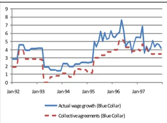
The specification (1) is general enough to comprise the predictions of most wage-setting models. It is evident that a spot labor market without frictions or bargaining leaves no role for firm-specific productivity to affect wages, once local labor mar-ket conditions have been accounted for. In contrast, wage bargaining models or models featuring search and matching frictions predict a positive effect from firm productivity on wages. In this context, the structure of wage bargaining is likely to be important. If wage negotiations between worker and employer associations take place at a sectoral level, productivity developments that are shared within sectors are likely to have a different impact on wages than purely idiosyncratic productivity. Wage negotiations in Sweden during our period of study were characterized by sectoral bargaining with an important presence offirm-level wage drift (see Appendix A). Hence, in the analysis we allow for both idiosyncratic and sector productivity to have an impact on wages. Conceptually, we can think of a two-stage, reduced-form model where sectoral wages () are set according to the average productivity in

the sector (

). Thereafter, firm-level wages () are determined by the firms’

idiosyncratic deviations from the sectoral means ( −). In order to account

for other factors, we may allow for common time effects (_), time-invariant sector specific () and firm-specific () effects, and local labor market tightness (()).

In (log) linear form:

 = 1+++

 = + (−)2+()++ (2)

The system naturally decomposes movements in labor productivity into a sec-toral and a firm-specific component with potentially different effects on wages. In order to arrive at the empirical specification which we estimate on worker-level wage

data, we add individual characteristics () and allow thefirm-specific fixed effect

to vary over individuals. Using the notation_ for the firm’s purely idiosyncratic productivity component (i.e.,_ =−), we propose the following empirical

specification:

=1+2+()+ +++ (3)

our parameters of interest being₁ and₂, which measure the responses of wages to sectoral (_) and idiosyncratic labor productivity (_), respectively. Note that the match-specific fixed effect () also captures all sector and firm-level fixed factors.

We estimate different versions of this model with different sets of control variables, for various subsamples, and we also let the effects of productivity vary across different types of firms and workers.

All our specifications include time effects, time-varying individual characteristics and labor market tightness at the local labor market. Similarly, we always include firm- (or match-) level fixed effects, since the TFP series we use to instrument la-bor productivity are derived from integrated firm-level changes, which produce an unknown constant for each firm (see details below). Firm effects also take care of anyfirm-specific characteristic that remains constant over the period of observation, helping to eliminate possible omitted variable biases at thefirm level. For instance, good working conditions may have a positive impact onfirm-level productivity, while at the same time these amenities would have a negative impact on wages if com-pensating wage differentials are important.5 This would then introduce a downward bias in our estimates of productivity on wages. To the extent that working condi-tions and other amenities do not change in the short period of time we are studying, they would be captured by the firm-level fixed effects.

Worker fixed effects eliminate possible composition biases associated with sys-tematic changes in the labor force of thefirm that are unobservable to the econome-trician. For instance, if high productivityfirms tend to attract high ability workers, and high ability workers are paid higher wages, our estimates of the effects of produc-tivity might be upwardly biased without individual fixed effects. The simultaneous account for worker and firm fixed effects therefore eliminate possible biases from sorting on either side of the market, but the average quality of retained matches can also change as a consequence of changes in productivity. For instance, poor matches may be thefirst to be dissolved in response to negative productivity shocks. In this case, what we interpret as the effects of productivity on wages might be driven by the sorting of bad and good quality matches that goes together with movements in productivity. We therefore include worker by firm match fixed effects in our most stringent specification. These eliminate observed and unobserved components of worker-, firm-, or match- specific heterogeneity and thus fully account for the sorting and matching of workers andfirms.

When estimating the impact of productivity on wages it is important to note that movements in labor productivity will capture both movements along the production function and shifts in the production function. Changes in product demand and factor prices may alter the scale of production and the capital-labor ratio and thereby affect labor productivity. Hence, OLS estimation of equation 3 may suffer from both omitted variables, since demand shocks in combination with decreasing returns may simultaneously alter productivity and wages if the labor supply curve is upward sloping, and endogeneity, since wage shocks may affect productivity through changes in the scale of production and/or factor proportions. Technological progress, if appropriately mapped by physical TFP, shifts the production function providing an

exogenous source of fluctuations in labor productivity. Hence, our strategy is to use a well-defined measure of firm-level TFP as an instrument for firm-level labor productivity. Next, we turn to the derivation of the TFP series.

2.2

Measuring TFP

We use a production-function approach to derive our technology series. The un-derlying idea is that technology can be measured as the residual from a production function once changes in both stocks and variable utilization of the production fac-tors are accounted for. We start by postulating the following production function forfirm:

 =(      ) (4)

where gross output  is produced combining the stock of capital , labor 

energy  and intermediate materials . The firm may also adjust the level of

utilization of capital,and labor,. Finally,   is the index of technology

that we want to capture.

2.2.1 Measuring TFP: Derivation

Using small letters to denote logs, taking the total differential of the log of (4) and invoking cost minimization, we arrive at:

∆=[∆+∆] +∆  (5)

where ∆ is the growth rate of gross output and  the overall returns to scale.

Denote as the cost share of factor  in total costs. Then, ∆ is a cost-share

weighted input index defined as ∆+∆+∆+∆.

∆.6 Thus, given data on factor compensation, changes in output, input and

utilization, and an estimate of the returns to scale_, the resulting residual∆ 

provides a times series of technology growth for thefirm. Note that∆  reduces

to a gross-output Solow residual if_ = 1,∆ = 0,∀ and there are no economic

profits.7 Hence, ∆  is a Solow residual purged of the effects of non-constant

returns, imperfect competition, and varying factor utilization.

In order to properly identify the contribution of technology, it is also important to distinguish between employees with different levels of education. Hence, using the same logic as above, we define ∆ as

∆ =∆ +∆ + ∆   (6)

where superscript   and   denotes workers with less than high school education, high school education and tertiary education, respectively, and _

denotes the cost share of category workers in total labor costs, where  _∈

{   _}. Hence, our labor input index will capture changes in the skill composition of the workforce of thefirm.8

The main empirical problem associated with (5) is that capital and labor uti-lization are unobserved. A solution to this problem is to include proxies for factor utilization. Here, we follow the approach taken by Burnside, Eichenbaum, and Re-belo (1995), who use energy consumption as a proxy for theflow of capital services. This procedure, which is well suited for our manufacturing sector data, can be

legit-6_{Here, the cost shares are assumed to be constants. We will return to this assumption later.} 7_{The zero-profit condition implies that the factor cost shares in total costs equal the factor cost}

shares in total revenues, which are used when computing the Solow residual.

8

We are, however, not accounting for the contribution to production of the unobservable skills of workers. Note that this is not a problem for the estimation of eq. (3) as long as the specification includes workerfixed effects.

imized by assuming that there is a zero elasticity of substitution between energy and theflow of capital services. This, in turn, implies energy and capital services to be perfectly correlated.9 Assuming that labor utilization is constant,10 and including a set of time dummies to capture any aggregate trends in technology growth ()

we arrive at the empirical specification used to estimate technology shocks

∆ =∆e++∆  (7)

where input growth, ∆_e, is defined as (+)∆+∆+∆.

Note that ∆  encompasses any firm-specific constant/drift term.

2.2.2 Measuring TFP: The importance of getting the measures right

Our key identifying assumption in the IV estimation of equation (3) is that TFP is exogenous to individual wages, and only affects wages through labor productivity. Here we illustrate some of the details of the empirical implementation of TFP, and we discuss why some of these details are crucial for this condition to be met. Funda-mentally, we show how using alternative measures of TFP based on sector deflated output or value-added rather than gross output would yield an invalid instrument.11 A first point is that it is crucial that nominal output is deflated by appropriate firm-level prices and not by sectoral price indices as is customary. We usefirm-level prices aggregated from unit prices for each good the firm produces (see Section 3

9

In Section 4.6 we examine the impact of using an alternative TFP series derived from estimates of the capital stock, where we can relax the Leontief assumption.

1 0_{In a related paper, Carlsson (2003) experiments with using various proxies for labor utilization}

(hours per employee, overtime per employee and the frequency of industrial accidents per hour worked) when estimating production functions like equation (7) on Swedish two-digit manufacturing industry data. Including these controls has no discernible impact on the results.

for further details), allowing us to derive true volume measures from gross output at thefirm-level. Following Klette and Griliches (1996), the problem with the usual approach, which uses a sectoral price index () instead of a firm-level price

index () can easily be seen by noting that the measure of real output deflated

by sectoral prices would be ln () = ln + ln() Hence, real

output deflated by sectoral prices would be a function of relative prices. Assume next that thefirm faces a constant elastic demand function, and sets its price as a (constant) markup over marginal cost as in the standard monopolistic-competition model. Since marginal cost, under standard assumptions, is proportional to unit labor cost, the relative price will be a function of wages (see Carlsson and Nord-ström Skans (Forthcoming), for direct empirical evidence). Importantly, this implies that sales deflated by sectoral pricesln ()and consequently also the

la-bor productivity and TFP measures derived from it, will respond to idiosyncratic wage shocks. The relationship between sector-deflated labor productivity (or TFP) and wages would then produce upwardly biased estimates of the causal impact of productivity on wages, even if firms are wage takers and produce according to a constant returns to scale technology (in which case marginal cost is independent of the scale of the production).

A second point is that gross output, as opposed to value-added, should be used as the output measure. TFP series derived from standard measures of value-added are only valid under perfect competition and constant returns. Instead, as shown in Appendix C, in the case of decreasing returns to scale a TFP measure derived from value-added would be negatively correlated with the growth rate of primary inputs. The drawback from this negative correlation can be easily illustrated in an example. Suppose there is a positive demand shock and the firm has decreasing

returns. Profit maximizing firms are likely to respond by increasing production, pushing up the demand for labor, electricity and other intermediate goods. As a consequence of decreasing returns, measured TFP based on VA will decline. If the demand shock has a positive impact on wages, for instance due to an upward sloping labor demand curve, we then expect a negative bias in the wage regressions.

Finally, we use electricity consumption to proxy for variations in the use of capital services as suggested by Burnside, Eichenbaum, and Rebelo (1995). Although this may not be optimal in all settings, it should provide a good approximation for the manufacturingfirms we study. The alternative would be to estimate capital stocks using the perpetual inventory method. A disadvantage of this alternative, in finite samples, is that it would require book values as starting values and these may be poor proxies for physical capital since they tend to be strategically constructed for tax purposes. Using electricityflows also has the advantage that it accounts for the actual use of the capital stock, i.e. theflow of productive services from capital, since electricity consumption responds to both capital utilization and changes in the stock of capital.

The empirical importance of these measurement issues are all thoroughly exam-ined in Section 4.8.

2.2.3 Measuring TFP: Empirical implementation

When empirically implementing specification (7), we take an approach akin to the strategy outlined by Basu, Fernald, and Shapiro (2001). First, the specification is regarded as a log-linear approximation around the steady state. Thus, the prod-ucts _ (i.e. the output elasticities) are treated as constants.12 Note that using

1 2

Given that we cannot observe thefirms’ capital stock to any precision, we cannot construct a credible direct measure of thefirms’ total capital cost, either. This, in turn, precludes the use of

constant cost shares (including the cost share of labor) precludes variation in wages to spill into variation in the TFP measure if, for any reason, _  is an

imper-fect measure of the output elasticity of labor input. Second, the steady-state cost shares are estimated as the time average of the cost shares for the two-digit industry to which the firm belongs (SNI92/NACE). Third, to calculate the cost shares, we assume thatfirms make zero profit in the steady state.13 Taking total costs as ap-proximately equal to total revenues, we can infer the cost shares from factor shares in total revenues. The cost share of capital and energy is then given by one minus the sum of the cost shares for all other factors.

Note that the estimation of equation (7) cannot be carried out by OLS, since the firm is likely to consider the current state of technology when making its in-put choices.14 We exploit the panel nature of our firm-level data to use internal instruments, as described in Section 4.

Once the series of technical change has been obtained following equation (7), the next step consists of integrating the growth rates in technology into a (log level) a Törnqvist-type (second-order) approximation relying on time-varying cost shares. However, the negligible effects reported in Carlsson (2003) from using time averages relative to time-varying cost shares indicate that this is not crucial.

1 3_{Using the data underlying Carlsson (2003) we find that the time average (1968}

−1993) for the share of economic profits in aggregate Swedish manufacturing revenues is about−0001. Thus, supporting the assumption made here.

1 4_{This is the so-called transmission problem in the empirical production function literature.}

Tech-nology change (i.e. the residual) represents a change in a state variable for thefirm and changes in the level of production inputs (the explanatory variables) are changes in thefirm’s control variables, which should react to changes in the state variable. In this case there will be a correlation between the error term and the explanatory variable, hence the need of IV methods.

technology series using the following recursion   = 0+ = X =1 ∆  (8)

Note that the initial level of technology ( 0) is a firm/sector-specific constant that is not observed, but will be captured by firm fixed effects in the second stage estimation.

2.3

Sector vs. idiosyncratic productivity

In the empirical specification of equation (3) we distinguish between sectoral

³

_

´

and idiosyncratic ³_´labor productivity. These measures can easily be obtained by running a regression of firm-level labor productivity, measured as gross output per worker, on sector-specific time dummies. The projection from the sector-specific time dummies in this regression is then a measure of 

, and the residuals are

a measure of _. We use employee weights when running this decomposition, such that sector-specific productivity is the average employee-weighted productivity, and idiosyncratic productivity is the firm-level deviation from this average. In an analogous fashion, we decompose the TFP series derived from (8) into a sectoral and an idiosyncratic TFP component.

3

Data

We combine three data sources to construct our sample. The employer side of the data set is primarily drawn from the Statistics Sweden Industry Statistics Survey (IS) and contains annual information for the years 1990-1996 on inputs and out-put as well as geographical location for all Swedish industrial (manufacturing and

mining) plants with 10 employees or more and a sample of smaller plants (see Ap-pendix B for details).15 Here we focus on continuing single-plant firms. Excluding multi-plant firms avoids the problem of identifying in which establishment of the firm technological change originates. The focus on continuing plants helps us deal with possible selection effects due tofirm demographics associated with productivity shocks.

A crucial feature of IS is that it includes a firm-specific producer price index constructed by Statistics Sweden. The firm-specific price index is a chained index with Paasche links that combines plant-specific unit values and detailed disaggre-gate producer-price indices (either at the goods level, when available, or at the most disaggregate sectoral level available). Note that in the case in which a plant-specific unit-value price is missing (e.g., when the firm introduces a new good), Statistics Sweden uses a price index for similar goods defined at the minimal level of aggrega-tion (starting at 4-digits goods code level). The disaggregate sectoral producer-price indices are only used when a plausible goods-price index is not available. Thus, the concern raised by Klette and Griliches (1996) regarding biased returns to scale esti-mates when sectoral price deflators are used in the computations of real gross output should not be an issue here.

The employee side of the data is obtained from the Register Based Labor Market Statistics data base (RAMS) maintained by Statistics Sweden. This data contains information on annual labor earnings for all privately employed workers in Sweden. The raw data was compiled by the Swedish Tax Authority in order to calculate taxes. The data includes information on annual earnings, as well as the first and last remunerated month received by each employee from each firm. We use this

1 5_{The availability of detailed factor input data, specifically electricity consumption, which are}

information to construct a measure of monthly wages for each employee in each of thefirms in our sample. The data lacks information on actual hours, so in order to restrict attention to workers reasonably close to full time workers we only consider a person to be a full-time employee if the (monthly) wage exceeds75percent of the mean wage of janitors employed by municipalities.16 We only include employment spells that cover November following the practice of Statistics Sweden. We focus on primary jobs and therefore only keep the job resulting in the highest wage for workers with multiple jobs. The data also includes information on age, gender, education, and immigration status of the individual workers.

Unemployment and vacancy data at the local labor market level for November is collected from the National Labor Market Board (AMS). Here, we rely on the 1993definition of homogenous local labor markets constructed by Statistics Sweden using commuting patterns, which divide Sweden into109geographic areas.

Note that we use the labor input measure available in IS to compute labor productivity, whereas the labor input measures used when estimating TFP are taken from RAMS. As mentioned above, the IS employment data is based on a survey collected by Statistics Sweden, whereas the RAMS employment data is based on the income statements that employers are, by law, required to send to the Swedish Tax Authority. Since the IS and RAMS measures of labor input are independently collected it is very unlikely that any measurement errors are common in the two. This, in turn, is important for ruling out that any observed relationship between labor productivity and technology is only due to common measurement errors in

1 6

Using a similar procedure with RAMS data, Nordström Skans, Edin, and Holmlund (2009) found that this gives rise to a computed wage distribution that is close to the direct measure of the

wage distribution taken from the3percent random sample in the LINDA database, where hourly

the labor input measures.

Both RAMS and IS provide unique individual and firm identifiers that allow us to link the employees to each of the firms in the sample. Since the RAMS data covers the universe of workers, we observe every worker employed in each of the IS firms during the sample period. Given the restrictions mentioned above and after standard cleaning procedures (see Appendix B for details), we are left with a balanced panel of 1136 firms observed over the years 1990-1996 and 472555 employee/year observations distributed over106050individuals. Our used data set cover about 10 percent of the total manufacturing sector.

4

Estimation results

4.1

Estimating TFP

Wefirst estimate the technology disturbances relying on the empirical specification (7) outlined in section 2 above. Here, we allow the returns to scale parameter_ to vary across durables and non-durables sectors as suggested by Basu, Fernald, and Shapiro (2001). The models includefirmfixed effects, which capture any systematic differences across firms in average technology growth. Since the firm is likely to consider the current state of technology when making its input choices, we need to resort to an IV technique. Following Carlsson and Smedsaas (2007) and Marchetti and Nucci (2005), we use a difference GMM estimator developed by Arellano and Bond (1991) and report robust, finite-sample corrected, standard errors following Windmeijer (2005). Here we use∆_e−, for≥3as instruments and collapse the

instrument set in order to avoid overfitting (see Roodman, 2006).17

1 7

Given that we use a difference GMM estimator, the second and higher ordered lags of ∆

Table 1: Returns to Scale Regression Industry RTS Durables 0.986 (0.194) Non-Durables 0.882 (0.224) AR(2) [0.210] AR(3) [0.886] Hansen [0.296]

Note: Sample 1991-1996 with 1,136

firms. Difference GMM second-step

es-timates with robust Windmeijer (2005)

finite-sample corrected standard errors in

parenthesis. See main text for

instru-ments used. Regression includes time

dummies andfirmfixed effects. P-values for diagnostic tests inside brackets.

In Table 1, we present the estimation results for equation (7). The estimate of the returns to scale for the durables sector equals 099 and 088 for the non-durables sector, but both are somewhat imprecisely estimated (s.e. of019and022, respectively).18 It is reassuring to see that the point estimates of the returns to scale are very similar to estimates reported by earlier studies. For example, Basu, Fernald, and Shapiro (2001) reports estimates of103and078for durables and non-durables, respectively, using U.S. sectoral data. Moreover, the Hansen test of over-identifying restrictions cannot reject the joint null hypothesis of a valid instrument set and a However, when including the second lag in the instrument set, the Hansen test of the over-identifying restrictions is significant at thefive-percent level.

1 8_{The data does not allow us to identify the returns to scale parameter separately across two-digit}

correctly specified model.

Importantly, Table 1 show that the AR(2) test of the differenced residuals indi-cates that there is no serial correlation in the estimated technology change series. This implies that we can regard these changes as permanent innovations to the technology level. The fact that our shocks in general appear to be of a permanent nature is consistent with the view that changes in TFP are capturing shifts in the production function. This should however be kept in mind when comparing our results with previous literature (e.g. Guiso, Schivardi, and Pistaferri (2005)), where the role on wage determination of temporary vs. permanent shocks to sales has been evaluated.

4.2

The impact of productivity on wages

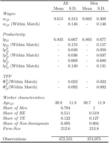
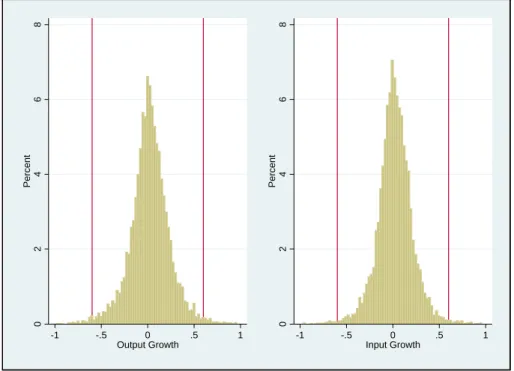
Before moving into the main results of the paper, we provide a brief description of the distribution of wages, TFP and labor productivity. Summary statistics are available in Table 2. First of all note that the dispersion of productivity is much wider than the dispersion of wages, but that this relationship is to a large extent driven by large differences betweenfirms. The variance (over time) within an employment spell (i.e. a match between a worker and afirm) is about equal. In the analysis we distinguish between a sectoral and an idiosyncratic component as discussed above. The sectors are identified following the 16 employer federations that sign collective agreements in the manufacturing sector.1920 When decomposing productivity within and between sectors we see that the within-match standard deviation of idiosyncratic firm-level productivity is nearly three times larger than the variance of sectoral productivity.

1 9

In practice we allocate thefirm to the most common employer federation amongfirms in the

samefive-digit industry according to the standard NACE classification.

Table 2: Summary Statistics All Men Mean S.D. Mean S.D. Wages:  9.615 0.313 9.662 0.308  (Within Match) - 0.146 - 0.146 Productivity:  6.835 0.667 6.865 0.677  (Within Match) - 0.155 - 0.157 _ - 0.049 - 0.050 _ (Within Match) - 0.036 - 0.037   - 0.669 - 0.680 _ (Within Match) - 0.130 - 0.131 TFP Φ (Within Match) - 0.022 - 0.022 Φ_(Within Match) - 0.092 - 0.092 Worker characteristics:  39.8 11.8 39.7 11.9 Share of Men 0.794 1 Share of HE 0.511 0.519 Share of TE 0.122 0.127 Share of Non-Immigrants 0.895 0.904 Firm-Size 212.6 213.8 Observations 472,555 374,975

Note: The "Within match" rows shows the dispersion within a combi-nation of person andfirm. All statistics are weighted according to the number of employees.

We proceed by investigating the role of sectoral andfirm idiosyncratic productiv-ity on individual wages, following equation 3. Thefirst column in Table 3 shows the results of estimating a simple OLS regression that relates labor productivity to in-dividual wages controlling forfirm-levelfixed effects, but excluding worker controls. Column 2 shows the same specification, now using idiosyncratic and sector-level TFP as instruments for the two labor productivity measures. Column 3 adds a third-order age polynomial and worker fixed effects. Column 4 presents our most stringent specification, including match-specific fixed effects. Column 5 repeats the last exercise for males. Standard errors are robust to intra-firm correlation.

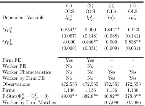
Both firm-level idiosyncratic labor productivity and sectoral labor productivity matter for wage determination. However, in order to obtain this conclusion it is fundamental to instrument the labor productivity measures, at least with regards to the sector-specific productivity. The OLS results in column 1 suggest a positive and statistically significant impact of idiosyncratic labor productivity on wages, with an elasticity of 0033 The estimated coefficient of the sector-specific productivity presents a similar magnitude (0027), but is not statistically different from zero. In sharp contrast, when we use TFP to instrument the labor productivity measures in column 2, wefind an elasticity of wages to sectoral productivity that is substantially larger than the elasticity with respect to idiosyncratic productivity,0123compared to0032. Both estimated coefficients in column 2 are statistically significant at the 1% level.21 _{We will return to a discussion below of potential explanations for why} the sectoral OLS results may be downwardly biased. Table 4 shows the first-stage regressions. The values of the F statistics are well above 10, suggesting that our instruments are not weak. More importantly, the Kleibergen-Paap rk LM statistic

2 1_{In a similar vein, Fuss and Wintr (2009)finds that aggregate wages per employee at thefi}

Table 3: The Impact of Productivity on Individual Wages. OLS and IV Results

(1) (2) (3) (4) (5)

Estimation Method: OLS IV IV IV IV

Sample: All All All All Males

_ 0.027 0.123** 0.149** 0.149** 0.149**

(0.022) (0.036) (0.037) (0.038) (0.041)

_ 0.033** 0.032** 0.050** 0.051** 0.054**

(0.008) (0.011) (0.010) (0.010) (0.011)

Firm FE Yes Yes Yes — —

Worker FE No No Yes — —

Worker Characteristics No No Yes Yes Yes

Match Specific Fixed Effects No No No Yes Yes

Observations 472,555 472,555 472,555 472,555 374,975

Firms 1,136 1,136 1,136 1,136 1,136

Kleibergen-Paap rk LM statistic - 46.83 NA 44.52 39.94

P-value - 0 NA 0 0

Worker*Firm Matches - - - 107,086 82,702

Note: * (**) denotes significance at the 5 (1) percent level. Standard errors clustered onfirms reported inside parentheses. All specifications include time effects and labor market tightness. Individual controls include age, age squared and age cubed (columns 3-5). K-P denotes the Kleibergen-Paap (2006) rk LM statistic for testing the null hypothesis that the equation is un-deridentified. P-value denotes the associated p-value for the test.

(see Kleibergen and Paap (2006)), presented at the bottom of Table 3, clearly reject the null hypothesis of underidentification.22

The rest of Table 3 shows that the results are somewhat larger when we include covariates that capture the skills and qualities of workers and indicators of match quality. Column 3 accounts for individual observed and unobserved heterogeneity by

2 2_{Note that the fact that thefirst stages are close to unity suggests that the endogenous response}

in input usage is small. This is reassuring since we are using a balanced panel and, due to the relatively short period available, are unable to model exits offirms.

Table 4: First-Stage Regressions

(1) (2) (3) (4)

OLS OLS OLS OLS

Dependent Variable: _ _ _ _

 _ 0.854** 0.000 0.842** -0.020

(0.087) (0.148) (0.088) (0.141)

 _ -0.000 0.846** 0.000 0.838**

(0.008) (0.031) (0.009) (0.031)

Firm FE Yes Yes — —

Worker FE No No — —

Worker Characteristics No No Yes Yes

Worker by Firm FE No No Yes Yes

Observations 472,555 472,555 472,555 472,555

Firms 1,136 1,136 1,136 1,136

F-Stat(Φ

=Φ = 0) 49.00** 382.8** 46.82** 378.8**

Worker by Firm Matches - - 107,086 107,086

Note: * (**) denotes significance at the 5 (1) percent level. Standard errors clustered on firms reported inside parentheses. Regressions also include time effects and labor market tightness. Individual controls (columns 3-4) include age, age squared and age cubed. F denotes the F statistic for the excluded instruments.

means of an age polynomial and individual fixed effects. The idiosyncratic compo-nent increases to0050, while the sectoral component increases to0149. The results are virtually identical if worker and firm effects are replaced by worker-firm match fixed effects, as shown in column 4. The latter may be a result of the fact that we are using a fairly short panel and only a subset of the economy, which means that the individualfixed effects in many cases are identified from single spells (i.e. that the matchfixed effects are already captured in the model with worker andfirmfixed effects).23

2 3

Our data does not allow us to properly control for part-time work, but since part-time work in Sweden is very rare among males in the manufacturing sector we have reestimated the model using only males. Column 5 presents results for the male sub-sample. The estimates show that the response of male wages to changes in productivity is very similar to that obtained in the overall sample. The elasticity of wages to sectoral productivity is almost three times as large as the elasticity to idio-syncratic movements in productivity, both estimates being statistically significant at standard levels of testing.

Albeit the estimated elasticities are far from unity, one must bear in mind that the variance of the underlying productivity processes is relatively large. This is es-pecially true in the case of idiosyncraticfirm-level productivity. Removing variation betweenfirms and using our preferred estimates in column 4 of table 3, wefind that an increase of one standard deviation in either of the productivity measures (sector or idiosyncratic) raises wages by about one quarter of the averagereal wage growth in our sample.24

For this purpose, we parallel the specification in column 4 of Table 3 and estimate the impact of

TFP on wages using OLS. Wefind marginally smaller effects on wages than those reported in Table

3 (0124and0042respectively). This is not surprising, considering that the thefirst stage of the IV regressions (Table 4) showed estimates of the TFP components somewhat smaller than unity. This model is, however, more sensitive to potentially attenuating measurement errors.

2 4

Average real wage growth within the manufacturing establishments included in the sample is 2.4%. Considering that our estimates are conditional on time effects, the estimated elasticities should be read as the impact of the different productivity components on real wages. Hence, the es-timated impact of one s.d. idiosyncratic productivity on wages amounts to 28% (0.051*0.130/0.024)

of the average real wage growth, while the impact of one s.d. sectoral productivity is 22%

4.3

Returns to scale, OLS and IV

The estimated impact of sectoral productivity developments on wages in the IV specifications is much larger than in the OLS regressions. A simple yet plausible explanation for such differences is attenuation bias due to measurement errors, but in that case it would be expected that there is a similar gap between IV and OLS estimates for the idiosyncratic productivity shocks. As this bias was not found, our results are most likely indicative of an endogenous negative association between labor productivity and wages at the sectoral level, which we try to examine next.

One straightforward explanation is a combination of decreasing returns to scale and an upward sloping labor supply curve, the intuition being that whenfirms choose to scale up production (e.g., in response to demand shocks) they will endogenously lower labor productivity if returns to scale are decreasing. The resulting increase in demand for labor will lead to higher wages if the supply curve facing the sector (or firm) is upward sloping. This may explain why instrumentation matters specifically at the sectoral level and not at the idiosyncratic firm level, since wages may be pushed up more in response to sectoral adjustments iffirms within a sector compete over a restricted set of workers. Hence, increased demand for labor within a sector may raise wages while single firms may be allowed to hire freely without affecting wages in the market. Naturally, differential wage responses to increases infirm labor demand versus sectoral labor demand may be reinforced by sectoral bargaining.

While the combination of decreasing returns with an upward sloping wage set-ting curve is consistent with our main results, we also try to provide a piece of somewhat more direct evidence by tentatively investigating the role of returns to scale. As shown previously, estimated returns to scale vary between the manufac-turing plants producing durable goods (decreasing returns) and those producing

non-durables (almost constant returns). Although our estimates of the returns to scale are imprecise, similar differences between durables and non-durables have been previously found in the literature (e.g. Basu, Fernald, and Shapiro (2001)). Hence, we expect the gap between IV and OLS estimates for sectoral productivity to be larger in firms operating in durable goods sectors than in firms operating in the non-durables sectors.

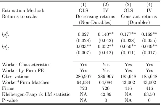
In Table 5 we estimate our preferred model (i.e. with match-specificfixed effects) using OLS and IV separately, for firms with decreasing and constant returns. The results are consistent with the proposed hypothesis. The entire difference between the sectoral OLS and IV estimates stems from the firms facing decreasing returns in our sample, while differences within firms facing constant returns are negligible and non-statistically significant. In the case offirms with decreasing returns, we see that the elasticity of wages to sectoral shocks becomes highly significant and more than 4 times larger in the IV specification (014vs. 0027in OLS). Interestingly, we also see that instrumentation leads to a non-negligible increase in the estimate of the idiosyncratic productivity effects on wages (from an elasticity of 0033in the OLS specification in column 1 to 0052 in column 2).25 _{This suggests that aggregation} over the sectors also blurred an important role for scale adjustment in response to idiosyncratic productivity, in the sectors where returns are decreasing.

4.4

Bargaining power, outside options and sectoral productivity

advance-2 5

The differences between the IV and OLS elasticities in columns (1) and (2) are statistically significant at the 5% level. The p-values of one-sided tests are 0.044 in the case of idiosyncratic productivity and 0.004 in the case of sectoral productivity.

Table 5: OLS and IV with Decreasing and Constant Returns to Scale

(1) (2) (2) (4)

Estimation Method: OLS IV OLS IV

Returns to scale: Decreasing returns Constant returns (Non-Durables) (Durables)   0.027 0.140** 0.177** 0.169** (0.028) (0.042) (0.038) (0.055) _ 0.033** 0.052** 0.050** 0.049** (0.007) (0.012) (0.011) (0.017)

Worker Characteristics Yes Yes Yes Yes

Worker by Firm FE Yes Yes Yes Yes

Observations 286,907 286,907 185,648 185,648

Worker*Firm Matches 64,084 64,084 43,002 43,002

Firms 720 720 416 416

Kleibergen-Paap rk LM statistic NA 42.89 NA 63.50

P-value NA 0 NA 0

Note: * (**) denotes significance at the 5 (1) percent level. Standard errors clustered on

firms reported inside parentheses. All specifications include time effects and labor market tightness. Worker characteristics include age, age squared and age cubed. K-P denotes the Kleibergen-Paap (2006) rk LM statistic for testing the null hypothesis that the equation is underidentified. P-value denotes the associated p-value for the test.

ments are shared within a bargaining sector.26 This can be explained by two dif-ferent mechanisms. Firstly, workers’ bargaining power may differ depending on the level of negotiation. In practice, workers may have more bargaining power during sectoral negotiations, since strikes are illegal during local bargaining but not during sectoral bargaining (see Appendix A for a discussion). Secondly, the shocks that are shared within a sector also affect the outside option of workers (or equivalently, the quality of counterbids in a poaching game, as in Cahuc, Postel-Vinay, and Robin (2006)), strengthening their bargaining position. This may occur if workers are mo-bile within sectors clustered in certain geographic areas. In this case, an increase in the bargaining position of workers is expected to be higher if technology improves in all of thefirms operating in the same sector.

In order to disentangle the two forces outlined above, we re-estimated the model controlling for predicted outside wages.27 _{If the higher elasticity of wages to sectoral} shocks is due to an improvement in the outside option of workers, we expect the estimated elasticities to decline once an estimate of the outside option of workers is included in the regression.

We estimate the outside wages as the predictions from 763 local labor market (109 areas) and year-specific (7 years) wage regressions using information about age, gender, immigration status (7regions) and education (both four-digitfield and three-digit level codes building on ISCED 97). We do thesefirst-stage regressions for the universe of full-time primary employments in the private sector, which amounts

2 6_{Interestingly, this result does not seem to be related to the particular definition of the sector we}

use. We have experimented using standard definitions of sectors, following the NACE classification at a two-digit level instead of the employer confederation of thefirms, andfind very similar results.

2 7_{These estimates, however, might be endogenous, so the interpretation of these results should}

in our sample to 11523194 observations for2653639workers. As expected, re-estimating equation (3) controlling for these predicted wages (highly significant with an elasticity of 058) in the regressions reduces the impact of sectoral productivity (from 0149 to 0096), but a substantial difference between the idiosyncratic and sectoral estimates remains (0057). Moreover, the elasticity of wages to idiosyncratic productivity is much less affected by the inclusion of outside wages. The difference between the two elasticities is marginally statistically significant (p-value of 011). Taken at face value, these estimates suggest that the workers’ ability to extract larger rents from sectoral than idiosyncratic shocks is equally driven by the two mechanisms we postulated: stronger bargaining power and better outside options.

4.5

The role of dynamics

The specifications we have presented so far are static, i.e., they assume that the wage impact of technology-driven innovations in productivity is immediate. In reality, permanent technology shocks might require some time to be absorbed by wages, e.g., if wage bargaining takes place biannually. In order to assess the importance of potential delays in the impact of productivity, we have estimated models with lagged productivity.

Estimates from specifications with lagged productivity are presented in Table 6. We concentrate on our preferred specification (including match-specificfixed effects) and proceed parsimoniously, first introducing one lag in column 2 and two lags in column 3.28 The bottom of the table shows the long-run accumulated effect, and its associated level of significance. The results show that there is a role for lagged productivity in shaping current wages. The effect does, however, seem to deteriorate

2 8_{Given the short nature of our panel we were not able to estimate models with more than two}

Table 6: Dynamic Effects (1) (2) (3) Estimation method: IV IV IV _ 0.149** 0.052 0.226 (0.038) (0.095) (0.130) _−1 0.104 0.198 (0.088) (0.211) _−2 -0.122 (0.147) _ 0.051** 0.035** 0.033* (0.010) (0.012) (0.014) _−1 0.034** 0.032** (0.013) (0.012) _−2 0.026* (0.010)

Total Sector Effect 0.149** 0.157** 0.303**

s.e. (0.038) (0.045) (0.110)

Total Idiosyncratic Effect 0.051** 0.068** 0.091**

s.e. (0.010) (0.015) (0.020)

Worker Characteristics Yes Yes Yes

Worker by Firm FE Yes Yes Yes

Observations 472,555 402,058 335,291

Firms 1,136 1,136 1,136

Worker*Firm Matches 107,086 99,473 93,316 Kleibergen-Paap rk LM statistic 44.52 25.79 4.775

P-value 0 0 0.029

Note: * (**) denotes significance at the 5 (1) percent level. Standard errors clustered onfirms reported inside parentheses. All specifications include time effects and labor market tightness. Worker characteristics include age, age squared and age cubed. K-P denotes the Kleibergen-K-Paap (2006) rk LM statistic for testing the null hypothesis that the equation is underidentified. P-value denotes the associated p-value for the test.

fairly rapidly and in the case of sectoral productivity we neverfind the individual lags to be statistically significant. Although the individual lags are estimated with poor precision, the long-run elasticity remains statistically significant in all cases. The magnitude of the long-run impact is about twice as large as the contemporaneous impact for both the idiosyncratic effect (0091 vs. 0051) and the sectoral effect (0303vs. 0149) when two lags are considered.

4.6

Variations

A very active literature (Shimer (2005), Hall (2003), Pissarides (2007)) discusses why unemployment fluctuates so dramatically over the business cycle compared to the smooth movements in aggregate productivity. A key element in this debate is the exact modeling of howfirms react in their setting of wages for incumbents and new hires when productivity changes (Haefke, Sonntag, and Van Rens (2008)). We have analyzed the impact on incumbents and new hires of sectoral and idiosyncratic productivity, but found no significant differences in their impact. However, it should be acknowledged that the interacted estimates are quite imprecise. We have also investigated if productivity advances affect workers with different skills differently, againfinding no significant heterogeneity, although with poor precision. Finally, we have analyzed whether productivity has a differential impact depending on whether the shocks are positive or negative, where one might suspect that negative shocks have a smaller effect due to downward nominal wage rigidity. Wefind no evidence of such asymmetries. Although this may seem surprising, it should be noted that the magnitudes of the estimated elasticities are such that the wage impact of any “normal” shock is smaller than the average nominal wage increase among incumbent workers. This implies that there is indeed scope for a symmetric impact of positive

and negative productivity shocks, even if nominal wages never fall.

4.7

Productivity and the selection of workers

Our main estimates are only marginally affected by the inclusion of individual spe-cificfixed effects. This suggests that compositional effects throughfirm recruitment andfiring policies as a response to technology-induced changes infirm-level produc-tivity should be minor. In order to make this point more precise, we relate the level of productivity to measures of the employed workers’ earnings capacity.29

To this end, we first estimate a two-way fixed effects model with wages as the dependent variable, including person and firm fixed effects along the lines of the Abowd, Kramarz, and Margolis (1999) model (also including an age polynomial and year dummies), relying on data for the universe of full-time primary employments in the Swedish private sector during the period 1985-1989, i.e. the available years

before our sample.30 All in all, this amounts to8776223linked employer-employee observations. From the pre-sample estimations we extract the person effects, which we use as dependent variables in the same specifications that we used for our wage regressions.31

This analysis has two virtues. First, we use pre-dated data to estimate the person effects. Thus, the person effects are clearly exogenous to our innovations in technology. Second, our skill measure has the same scale as the wage, and the size of the selection responses can thus be compared to the endogenous wage responses.

2 9

See e.g. Abowd, Kramarz, Perez-Duarte, and Schmutte (2010) for an interpretation of esti-mated person effects in a structural matching framework.

3 0_{We use the Abowd, Creecy and Kramarz (2002) algorithm as implemented for STATA in a2reg}

by Amin Ouazad.

3 1_{Although the time span for estimating the person effects is short wefind a very high correlation}

Table 7: The Effects of Productivity on the Selection of Workers

(1) (2) (3) (4)

Estimation method: IV IV IV IV

Sample: All Less than High Tertiary

High School School Education

_ -0.024 -0.044* -0.001 -0.026

(0.015) (0.020) (0.018) (0.059)

_ -0.003 -0.001 -0.007 -0.008

(0.003) (0.004) (0.004) (0.009)

Firm FE Yes Yes Yes Yes

Worker Characteristics Yes Yes Yes Yes

Observations 417,870 161,954 207,236 48,675

Number of Firms 1,136 1,135 1,135 1,128

Kleibergen-Paap rk LM statistic 43.83 47.58 38.93 44.33

P-value 0 0 0 0

Note: The dependent variable is the person effect of the individual as extracted from a wage regression on person and establishmentfixed effects, an age polynomial, and year dummies for the entire private sector during 1985-1989. * (**) denotes significance at the 5 (1) percent level. Standard errors clustered onfirms reported inside parentheses. All specifications include time effects and labor market tightness. Worker characteristics include age, age squared and age cubed, a gender dummy, a high school dummy, a university dummy, immigration dummies by seven regions of origin. K-P denotes the Kleibergen-Paap (2006) rk LM statistic for testing the null hypothesis that the equation is underidentified. P-value denotes the associated p-value for the test.

Note also that any noise in the estimated person effects will be in the residual of the second-stage regressions, and thus only affect precision and not the point estimates. The results from the IV model includingfirmfixed effects are presented in Table 7. Column 1 shows the overall results, and columns 2 to 4 show separate estimates for samples of workers with less than high school education, high school-educated employees and workers who attended tertiary education, respectively. The estimates of the elasticity of the portable earnings capacities tofirm idiosyncratic and sectoral

productivity are very close to zero, in particular those relative to idiosyncratic pro-ductivity, and non-statistically significant. When we split the sample according to observable skills, we see a tendency toward negative assortative matching in response to sector-specific productivity in the group with the lowest skills.32 All estimates related to idiosyncratic productivity are tiny and non-different from zero at standard levels of testing. We have also experimented with productivity lags in this specifi ca-tion, but the effects remain insignificant and small. Overall, the analysis therefore suggests that the skill composition of workers within afirm is largely unaffected by changes in both sectoral and idiosyncratic productivity.

4.8

Measurement issues

In the main text, we have stressed the importance of using the right price measures to deflate output in the main text. Following our discussion in Section 2.2.2, wage shocks will transmit into measured real output series if sectoral prices are used when deflating sales to obtain real output, generating a positive bias in the estimated impact of idiosyncratic productivity. This conjecture is confirmed by the results presented in Table 8. The first column replicates our baseline results for the sake of comparison. In column 2, we use 3-digit PPI deflators instead offirm-level prices to derive gross output. Using sectoral deflators results in an estimated elasticity of idiosyncratic productivity of almost twice the size (0092) of the benchmark.

Two-3 2_{Interestingly, these estimates are in line with the conclusions in Abowd, Kramarz, Perez-Duarte,}

and Schmutte (2010), who estimate a structural job assignment model with coordination frictions. Theyfind that low ability workers have a comparative advantage in highly productivefirms within manufacturing, but that the empirical influence of sorting is minor because of limited heterogeneity. For results that instead pointing toward positive assortative matching and further references, see Mendes, Van Den Berg, and Lindeboom (2010).

sided tests show that this difference is statistically significant at the 1% level. As a second experiment, we show the impact of using a measure of value-added instead of gross output to derive the productivity and technology series.33 As dis-cussed in Section 2.2.2, the main problem with value—added based measures of TFP is that they will be negatively correlated with the intensity of the use of primary inputs, including labor, if there are decreasing returns to scale. Column 3 of Ta-ble 8 presents the results of using a value-added Solow residual to instrument for value-added labor productivity.34 We see that the value-added estimates are con-siderably smaller than those based on TFP, as expected if demand shocks have a positive impact on wages. The negative bias is somewhat larger for the sectoral e