CREDIT Research Paper
No. 01/14
_____________________________________________________________________
Problems with Pooling in Panel Data
Analysis for Developing Countries: The
Case of Aid and Trade Relationships
by
Tim Lloyd, Oliver Morrissey and Robert Osei
_____________________________________________________________________ Centre for Research in Economic Development and International Trade,
the School of Economics at the University of Nottingham. It aims to promote research in all aspects of economic development and international trade on both a long term and a short term basis. To this end, CREDIT organises seminar series on Development Economics, acts as a point for collaborative research with other UK and overseas institutions and publishes research papers on topics central to its interests. A list of CREDIT Research Papers is given on the final page of this publication.
Authors who wish to submit a paper for publication should send their manuscript to the Editor of the CREDIT Research Papers, Professor M F Bleaney, at:
Centre for Research in Economic Development and International Trade, School of Economics, University of Nottingham, University Park, Nottingham, NG7 2RD, UNITED KINGDOM Telephone (0115) 951 5620 Fax: (0115) 951 4159
CREDIT Research Papers are distributed free of charge to members of the Centre. Enquiries concerning copies of individual Research Papers or CREDIT membership should be addressed to the CREDIT Secretary at the above address. Papers may also be downloaded from the School of Economics web site at:
CREDIT Research Paper
No. 01/14
Problems with Pooling in Panel Data
Analysis for Developing Countries: The
Case of Aid and Trade Relationships
by
Tim Lloyd, Oliver Morrissey and Robert Osei
_____________________________________________________________________ Centre for Research in Economic Development and International Trade, University of Nottingham
Tim Lloyd is Lecturer and Internal CREDIT Fellow, Oliver Morrissey is Reader and Director of CREDIT and Robert Osei is a Research Officer, all in the School of Economics, University of Nottingham.
____________________________________________________________ July 2001
of Aid and Trade Relationships
by
Tim Lloyd, Oliver Morrissey and Robert Osei
Abstract
It is common practice in empirical development macroeconomics to use cross-country samples for econometric analyses. One issue that is rarely addressed in this literature is the appropriateness of pooling when panels are used. In particular, does it matter to the results if the countries exhibit different time series properties in respect of the relationship being observed? This is the issue addressed in this paper, taking the example of the ‘aid and trade’ relationship. We also address the following questions: (a) Is there any support for the assertion that donors use aid to perpetuate their trade with recipients? (b) How important is trade in influencing aid allocation decisions of donors? The principal result is that pooling countries with different underlying time series properties (different inherent causality) is inappropriate and gives misleading results. In other words large samples are not necessarily the best samples. Using appropriate samples, we find no evidence that tied aid increases trade, although donors providing a higher share of aid tend to trade more with the recipient. In terms of aid allocation, donors appear to be concerned with relative aid and trade shares rather than absolute volumes.
Outline
1. Introduction
2. Model Specification 3. Econometric Issues 4. Some General Issues 5. Results and Discussion 6. Conclusions
I. INTRODUCTION
It is common practice in empirical development macroeconomics to use cross-country samples for econometric analyses. Partly, the motive lies in the paucity of time series data available for adequate analysis, especially for the poorest countries. More generally, the justification lies in the claim that cross-country data at least allows one to identify aggregate relationships, or correlations in the data that appear to hold ‘on average’ over a wide sample. The weakness of this approach is that what appears to hold on average is rarely an adequate explanation of what is happening in a particular country. Furthermore, the macroeconomic relationships of interest are typically dynamic in nature, so that researchers should be interested in what is happening in countries over time. Cross-section techniques are limited in their ability to address this concern.
Increasingly, panel data techniques are employed to avail of the time series dimension and/or ‘smooth out’ year-on-year variability in the data. Examples abound in the literature, and it is not our intention to even attempt a review.1 However, results are often sensitive to the sample used,2 suggesting reason to question the generality of the ‘average’ relationship uncovered. One issue that is rarely addressed in this literature is the appropriateness of pooling the countries in the sample, especially when panels are used. Most studies, if properly conducted, will test for outliers and/or cross-section pooling (whether the observations appear to be from the same population). However, it is not common practice to try and test for what can be described as ‘time series pooling’ – does the underlying causal relationship appear to be the same for all countries.3 Of course, data
1 Burnside and Dollar (2000) is a recent example applying panel techniques to investigate the impact of aid on growth, and Borenzstein et al (1998) use such techniques to address the impact of FDI on growth. All such studies could be considered to be ‘nested’ within the empirical literature on the determinants of growth in developing countries. Despite numerous studies and enormous research effort, the results are disappointing: ‘the universal failure to produce robust, causally secure relations predicted by models might suggest … that country growth experiences have been extremely heterogeneous’ (Kenny and Williams, 2001: 12).
2 Hansen and Tarp (2001), for example, demonstrate that the Burnside and Dollar (2000) results are very sensitive to the choice of whether to include or exclude certain apparent outliers.
3 Some studies implicitly recognise this. For example, Chang and Ram (2000) split their sample into high-growth and low-high-growth countries to compare the evolution of inequality with respect to income. The difference is evident, with high-growth countries exhibiting a lower inequality at all income levels. Bahmani-Oskooee and Nasir (2001) use an econemtric technique that accounts for the time-wise
constraints may render it difficult to do this. Is this something about which researchers should be concerned? In particular, does it matter to the results if the countries exhibit different time series properties in respect of the relationship being observed? This is the issue addressed in this paper, taking the example of the ‘aid and trade’ relationship.
The ‘aid and trade’ relationship is particularly appropriate to our concerns because the link can be in either direction.4 On the one hand, trade (imports of the recipient from the donor) may be one indicator of economic ties between the donor and recipient. In this way, trade will be a factor in aid allocation, that is trade flows determine aid flows.5 Alternatively, aid may determine trade flows. This can happen directly, when the aid is tied (to imports from the donor), or indirectly, if the aid contributes to growth and an increase in the demand for imports from the donor. In either case, aid can be said to determine trade. For any given donor-recipient pair, either or both forces could be operating. It follows that in any panel, the observed aggregate relationship will depend on which of these effects dominates.
An implicit assumption often made in cross section and panel data analysis of the bilateral aid and trade relationship is that the nature of the relationship is invariant to the sample of donor-recipient pairs used. The norm has been to use the sample of donor recipient pairs for which data are available. As Lloyd et al. (2000) show, the exact nature of the relationship depends on the nature of causality between any donor-recipient pairs. They identify five cases for classifying bilateral aid and trade relationships. Case I is where trade
Granger-causes aid6, and this would be the implicit assumption for aid allocation studies.
Case II is where aid Granger-causes trade, as often assumed by donor policy-makers who
autogressive properties of the countries in their panel. The same technique is employed by Morrissey (2000) in a study of the aid-trade relationship examined here.
4 Recent reviews of the literature can be found in Cnossen et al (1999) and Lloyd et al (2000) so the discussion here is quite brief.
5 Poirine (1999) presents a novel variant on this theme by demonstrating that in certain cases aid is trade, where the aid is in effect payment for strategic assets (a non-market public good that the recipient has a comparative advantage in producing and which the donor demands). Examples include the high per capita aid transfers from the US and France to remote islands that provide military bases or nuclear testing facilities.
6 Granger Causality is a statistical concept describing when prediction of the current value of a variable, say yt, is improved by knowledge of the past values of another variable, say xt, and such historic information is unique to xt (Granger, 1988).
claim that aid creates exports. Combined scenarios are Case III where there is
bi-directional causation, Case IV where there is contemporaneous causation, and Case V
where no statistical relationship exists. Lloyd et al (2000) find instances of all five cases in a study of four major European donors and 26 African recipients.
The bilateral aid-trade relationship is an example of an economic relationship where the direction of causality between the variables of primary interest may differ among countries in the sample.7 It is therefore an example of what can be termed time-series heterogeneity. The primary objective of this paper is to investigate the effect of the presence of such heterogeneity on the results of panel estimation. Are there any significant gains from pre-testing the data to identify if the underlying causal relationship differs between countries in the sample? Using the example of the bilateral aid-trade relationship, we will argue that such heterogeneity does bias the results and countries exhibiting different underlying causal relations should not be pooled in a single panel.
We also address the following questions: (a) Is there any support for the assertion that donors use aid to perpetuate their trade with recipients? (b) How important is trade in influencing aid allocation decisions of donors? A few studies have addressed these issues in general. However this paper differs in one major way. The data we use for our study have been put into panels based on results from Granger-causality tests (Lloyd et al, 2000). This means that for the analysis of the aid leading to trade hypothesis we use a sample of donor-recipient pairs for which aid is found to Granger-cause trade. We use the sample of donor-recipient pairs for which trade is found to Granger-cause aid for analysis of the aid allocation hypothesis.
The organisation of the paper is as follows: In section 2 we discuss the theoretical underpinning of the model specifications used in the study. The econometric issues are discussed in section 3. Some general issues relating to the data and estimation procedures are discussed in section 4. Section 5 presents the results. The conclusions are given in section 6, where we argue that pooling does matter.
7 It is not difficult to think of other examples within the empirical growth literature for developing countries. Does aid cause growth or does growth cause aid? Do exports cause growth or does growth cause exports? Such concerns of causality and endogeneity are at the heart of empirical studies of growth.
II. MODEL SPECIFICATION
As causality between aid and trade flows can be in either direction, two general specifications are provided. The first sets out the factors of concern in the ‘aid to trade’ relationship. The second, based on aid allocation literature, sets out factors relevant to the ‘trade to aid’ relationship. Appropriate literature is referred to in discussing each.
Aid to Trade Relationship
The theoretical basis of the model used for this set of equations is similar to that of Nilsson (1997), with some modifications. Nilsson (1997) employs a version of the gravity model to analyse the effects of bilateral and multilateral aid on EU exports to recipient countries. The basic idea of the gravity model is that bilateral trade flows are explained by three sets of variables:
a) variables indicating total potential supply of the exporting country; b) variables indicating total potential demand of the importing country; and
c) variables that hinder or engender trade between importing and exporting countries. Some simplifying assumptions and these three sets can be reduced to two. We can classify most aid donors as ‘large countries’ and recipients as ‘small countries’, especially as we limit attention to Sub-Saharan African (SSA) recipients. This is because the export capacity of a typical donor exceeds the import capacity of the recipient. The ‘short-side rule’8 implies that it is the effective demand for a donor’s exports that is important in the aid to trade model. In the context of bilateral pairs, the recipients’ capacity to import determines the volume of trade rather than the donor’s capacity to export. Consequently, the model used in this paper to explain bilateral trade flows has two sets of variables (b and c above).
The physical distance between donor-recipient pairs is omitted as relative distance from Europe is unlikely to influence trade volumes between specific European and SSA
8 This rules states that if there is excess demand for a commodity then the quantity of the good bought is equal to the amount supplied. In like manner, under excess supply the amount bought equals that demanded (e.g. Benassy, 1986: 13).
countries (and does not vary over time). For trade with most African countries a major hindrance will be accessibility rather than physical distance from a given donor. Fixed effects estimation can attempt to account for the omission of such variables, especially as we measure variables in differences rather than levels.
The two types of equation estimated for this model are:
2 , 11 1 , 10 2 , 9 1 , 8 2 , 7 1 , 6 5 2 , 4 1 , 3 2 2 , 1 0 − − − − − − − − − + + + + + + + + + + + = t i t i t i t i t i t i it t i t i it t i it dish dish dash dash dlGnp dlGnp dlGnp dca dca dca dcim dcim β β β β β β β β β β β β (1) 1 2 2 1 1 1 2 1 6 5 4 3 2 1 2 , 11 1 , 10 2 , 9 1 , 8 2 , 7 1 , 6 5 2 , 4 1 , 3 2 2 , 1 0 dca D dca D dca D dca D dum dum dish dish dash dash dlGnp dlGnp dlGnp dca dca dca dcim dcim t i t i t i t i t i t i it t i t i it t i it γ γ γ γ γ γ β β β β β β β β β β β β + + + + + + + + + + + + + + + + + = − − − − − − − − − (2)
where βi’s and γj’s (∀ i,j ) are parametersand the variables are defined as follows:
dcim-t t-period lag of the change in imports of recipient from donor
dca-t t-period lag of the change in aid flows from donor to recipient
dlGnp-t t-period lagged per capita growth in GNP
dash-t t-period lag of change in the share of a recipient’s aid from a donor
dish-t t-period lag of the change in the share of a recipient’s imports from a donor
Dum1 A dummy that takes a value of 1 if the share of a recipient’s imports from a donor is at least equal to the sample mean, 0 otherwise
Dum2 A dummy that takes a value of 1 if the share of a recipient’s aid from a donor is at least equal to the sample mean, 0 otherwise
D1dca, etc. interactive terms, such as Dum1 × dca.
It is difficult in most cases to say a priori what the expected signs of the coefficients are. This is because there exists no formal theoretic model that seeks to explain the aid to trade relationship. Coupled with this is the fact that the literature abounds with numerous
hypotheses to explain the effect of these variables on bilateral trade. We discuss some of the main arguments also summarised in Table 1.9
The coefficient β2 should indicate the proportion of aid tied to trade and should have a positive sign with a magnitude of less than one. In the case of the coefficients on the lagged aid terms, β3 and β4, the sign is ambiguous. A positive effect could result if aid generates goodwill with the recipient and consequently leads to an increase in trade with the donor, so-called radiation effects of aid (Jepma, 1989). Another reason is when the tying of aid induces trade dependency. If aid is tied to donor exports then it increases the recipient’s exposure to goods and services from the donor in the form of follow-on orders (Cnossen et al, 1999). Another argument is through its impact on the macro economy. However in our model this argument will not be valid; the inclusion of output growth in the equation controls for the effect of aid on trade via growth. The net effect of aid on trade in equation (1) can be attributed to tying and its indirect effects only. Aid can also have a negative effect on trade. This can arise through the substitution effect of tied aid: as a result of tying, recipients buy from other countries goods they would have otherwise bought from the donor (Nilsson, 1997). One cannot say a priori what the net effect of aid will be in this equation.
Output growth should have a positive effect in any import demand function. This is also the implicit assumption made in the donor argument that aid creates trade through its impact on the macroeconomy. Growth is assumed to act as a proxy for the effective demand of the recipient. However, with bilateral trade flows this positive effect will not necessarily hold. Additional import demand need not benefit a specific donor. A negative relationship between output growth and bilateral trade between a particular donor-recipient pair could therefore be observed. Alternatively, if countries require capital goods produced by a specific donor imports from that donor may increase more than proportionally with output growth.
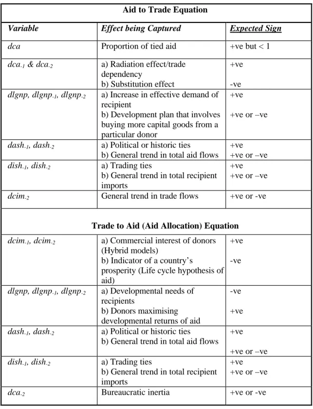
Table 1. Summary of the effects of variables in the models Aid to Trade Equation
Variable Effect being Captured Expected Sign
dca Proportion of tied aid +ve but < 1
dca-1 & dca-2 a) Radiation effect/trade
dependency
b) Substitution effect
+ve -ve
dlgnp, dlgnp-1, dlgnp-2 a) Increase in effective demand of
recipient
b) Development plan that involves buying more capital goods from a particular donor
+ve +ve or –ve
dash-1, dash-2 a) Political or historic ties
b) General trend in total aid flows
+ve +ve or –ve
dish-1, dish-2 a) Trading ties
b) General trend in total recipient imports
+ve +ve or –ve
dcim-2 General trend in trade flows +ve or -ve Trade to Aid (Aid Allocation) Equation
dcim-1, dcim-2 a) Commercial interest of donors
(Hybrid models)
b) Indicator of a country’s
prosperity (Life cycle hypothesis of aid) +ve -ve dlgnp, dlgnp-1, dlgnp-2 a) Developmental needs of recipients b) Donors maximising developmental returns of aid
-ve +ve
dash-1, dash-2 a) Political or historic ties
b) General trend in total aid flows
+ve +ve or –ve
dish-1, dish-2 a) Trading ties
b) General trend in total recipient imports
+ve +ve or –ve
dca-2 Bureaucratic inertia +ve or -ve
The share of a recipient’s aid from a donor can be thought of as representing some form of political or historic tie, implying a positive net effect of the aid shares on trade volumes.
An increase/decrease in aid share does not necessarily mean that aid volumes between any donor-recipient pair has increased/decreased; this depends on the trend in total aid receipts. The net effect of the aid shares could either be negative or positive. Import shares are also included in the equation as a proxy for trading ties between the pairs, implying a positive net effect of past levels of import share on current imports. The coefficient on the lagged trade terms could be either positive or negative depending on the general trend of trade flows between donors and recipients.
Equation (2) includes interactive terms to test for the structural stability of some of the parameters. The dummy variables test if the effect of aid on trade is the same if the share of aid (imports) a recipient gets from a donor exceeds some given threshold.10 This we do by examining the coefficients γ3 and γ4, (coefficients on the interactive import share dummy terms) and γ5 and γ6(coefficients on the interactive aid share dummy).
Aid Allocation (Trade to Aid) Equations
Empirical studies on aid allocation typically postulate three broad groups of variables as influencing donor allocation decisions (Lloyd et al, 1998 summarise the main studies; see also Poirine, 1999). These are classified as follows:
a) variables which capture the developmental requirements of the recipient;
b) variables which represents the recipient’s political and strategic importance to the donor, and
c) variables which represents the commercial and economic importance of the recipient to the donor.
Based on the above classification we estimate the following equations:
2 , 10 1 , 9 2 , 8 1 , 7 2 , 6 1 , 5 4 2 , 3 1 , 2 2 , 1 0 − − − − − − − − − + + + + + + + + + + = t i t i t i t i t i t i it t i t i t i it dish dish dash dash dlGnp dlGnp dlGnp dcim dcim dca dca δ δ δ δ δ δ δ δ δ δ δ (3)
10 This threshold is exogenous in the sense that it is the average share of aid (imports) in the sample of donor-recipient pairs for each panel. In other words it differs from sample to sample.
1 2 1 1 2 1 2 3 4 1 2 , 10 1 , 9 2 , 8 1 , 7 2 , 6 1 , 5 4 2 , 3 1 , 2 2 , 1 0 dcim D dcim D dum dum dish dish dash dash dlGnp dlGnp dlGnp dcim dcim dca dca t i t i t i t i t i t i it t i t i t i it λ λ λ λ δ δ δ δ δ δ δ δ δ δ δ + + + + + + + + + + + + + + = − − − − − − − − − (4)
where δi’s and λj’s (∀ i,j ) are parameters and the definition of variables are the same as defined for equations (1) and (2). Equation (4) includes interactive terms to test the stability of some of the parameters in equation (3). Namely, is the effect of trade on aid the same if the share of aid (or imports) a recipient gets from a donor exceeds some given threshold. The dummies are only allowed to interact with the trade terms in this equation. Lack of a formal theory makes it difficult to predict a priori the signs of the coefficients (Table 1 presents a summary of the expected signs of the coefficients). Most studies in the aid allocation literature have been based on ‘hybrid’ models that postulate a positive effect of trade on aid (see McGillivray and White 1993). In these models trade is a proxy for the commercial interest of donors. There are other theories which suggest that this effect could be negative. For instance Cnossen et al (1999) mention the life-cycle hypothesis of aid which argues that trade may be used as an indicator of a country’s prosperity. This means an increase in a recipient’s imports signifies that it is becoming more prosperous and so requires less aid.
Output growth is included to capture the development needs of a recipient; higher growth implies less need for aid. The expected effect of growth will in this case be negative. There is a counter-argument: Wittkopf is cited as arguing that if the concern of the donors is to maximise the developmental returns from aid then donors will give more aid to those countries with superior economic performance (McGillivray and White, 1993). Aid share is expected to have a positive effect as it is included to capture political ties. The effect may be weak in practice as an increase in aid shares may be associated with a decrease in aid flows between any donor-recipient pair.
Import shares will have a positive effect on aid if they capture the extent of trading ties between the pair. Donors are expected to give more aid to their trading partners. Most empirical work on aid allocation uses the level of trade to explain the level of aid (or explains aid shares using trade shares). It seems reasonable to expect donors to use trade
shares rather than levels to represent the potential. The lagged aid terms capture bureaucratic inertia (McGillivray and White, 1986): many projects extend over time and so aid bureaucracies use preceding year’s aid as a benchmark for current allocation. The coefficient on this term could be either positive or negative depending on the trend in aid flows.
III. ECONOMETRIC ISSUES
The general framework for the panel data analysis is a regression model of the form
yit = αi + βªxit + µit for i =1,2,…,N; and t = 1,2,…,T (5)
N and T are the cross section and time series dimensions respectively and xit is a vector of
K regressors. The vector of disturbance terms uit is assumed to be uncorrelated with the
xit’s and the αi’s have zero mean and constant variance, σu2. This model restricts the coefficients on x to be common across i and t. A less restricted form could allow the slopes to vary over time, across donor-recipient pairs or both.
The assumption made about αi has implications for the consistency and efficiency properties of estimates of β in equation (5). In an aid to trade equation the group-specific term reflects idiosyncratic preferences or characteristics of a donor-recipient pair. If the group-specific effect is assumed constant (but allowed to differ across units) the model is called a fixed effects (FE) model. Assuming heterogeneity across units in equation (5) implies that the effect of all omitted variables is the same for a given cross sectional unit through time but varies across cross-sectional units for a given point in time.
We employ one of two methods to estimate the model parameters in each equation. The choice of method is based on the efficiency and consistency properties of the resulting estimators. For the first method β’s are estimated by utilising the variation within each group, i. This makes use of the idea of partitioned regression. To see this rewrite equation (5) in terms of the group means:
Subtracting equation (6) from (5) yields ) ( ) ( ) (yit −yi• =β′ xit −xi• + µit −µi• (7)
OLS can then be used to estimate the β coefficients from equation (7). This is known as the within-group (WG) estimator. The WG estimator for β is unbiased and consistent when either N and/or T goes to infinity. An estimate for αi can be retrieved as the mean residual from the ith group, i.e.
t i i i y x β αˆ • ˆ •− = (8)
The estimator for αi from equation (8) above is unbiased but is consistent only when T
tends to infinity (Hsiao, 1986: 32).
The second estimator used in this paper makes use of the idea that heterogeneity across units can be accounted for by treating the individual specific effects as random variables. Here the assumption is that the unit specific effects cannot be observed or measured and so represents ‘specific ignorance’ for the modeller and must be treated as part of our ‘general ignorance’ (Matyas and Sevestre, 1992: 50). What this means is that the large number of factors that affect the value of the dependent variable but which are not explicitly accounted for in the model can be summarised by a random disturbance. If this assumption is made then we call it a random effects (RE) model. Hence in addition to a non-specific error term µit there is also a group-specific error term αi. Equation (5) is therefore written as
it it
it x
y =β′ +υ (9)
where νit = αi + µit and E(αi) = E(µit) = 0 ∀ i, t
Var(αi) = σα2 ; Var(µit) = σµ2 ∀ i, t
Cov(αi, αj) = 0 ∀ i ≠ j Cov(µit, µjs) = 0 ∀ i ≠ j, t ≠ s Cov(xit, αi) = 0, Cov (αi, µit) = 0
For the random effects model we still can use the WG estimator to obtain estimates
for β in equation (5) as the coefficients are time-invariant. This is obvious when one considers the transformation that yields equation (7). Note that in equation (7) the αi is absent and so estimating β's is independent of whether we assume a fixed effect or random effects model.11 The point worth noting here is that if we assume the αi's to be fixed then the WG estimator gives BLUE estimates. However if we assume αi's are random then in finite samples the WG estimator is consistent but not efficient. This inefficiency is due to the fact that we are not making use of the information that there is a group-specific random component in the equation error term (Hsiao, 1986: 34).
In equation (9), because both νit and νis (∀ s ≠ t) contain αi, the residual will be autocorrelated. An efficient estimator is therefore the GLS. The transformation that gets rid of this serial correlation is:
2 2 2 ) 1 ( ) 1 ( α µ µ σ σ σ θ θ θ T where x x x y y y i it it i it it + = − − = − − = • ∗ • ∗
The GLS therefore involves estimating by OLS the equation
it it
it x
y∗ =δ +β′ ∗ +ε (10)
where εit is a white noise error term.
It can be shown that the GLS estimator is a weighted average of the between-12 and within-group estimator and is given by the expression:
11 We would therefore not interpret the Wu-Hausman test (discussed below) as a test for random effects against fixed effects as most authors do; see for instance Green (1997).
BG xx xx xx WG xx xx xx GLS b w b b w w β θ θ β θ βˆ ˆ ˆ + + + = (11) 13
This compares with the OLS estimator given by
BG xx xx xx WG xx xx xx OLS b w b b w w β β βˆ ˆ ˆ + + + = (12) where 2 ) (
∑∑
− • = i t i it xx x x w 2 ) (∑∑
•− •• = i t i xx x x bThe OLS estimator just refers to estimating equation (5) with a pooled sample. Compared with the GLS estimator OLS places too much weight on the between-group variation (this is obvious when one compares the weights on the between- and within group estimates in equations (11) and (12)). All the variation is attributed to the variation in the independent variables X, instead of attributing some of it to random variation across groups, which is the role θ plays in equation (11). When there is no variation within the group-specific effects, i.e. σα2 =0, then we have θ = 1 which implies that βˆGLS =βˆOLS. Also as T → ∝, θ → 0 and therefore βˆGLS ≈ βˆWG.
The efficiency of the GLS estimator holds only if the independent variables (Xit) are uncorrelated with the random group-specific effects αi. This, as we discuss shortly, is the basis of the Wu-Hausman test.
In this paper two tests are reported and these form the basis of our choice between the WG and GLS estimator. The first is the Wu-Hausman test for the correlation between the
12 The between group estimator βBG, is the OLS of the regression which uses just the group means i.e. OLS on equation (2).
regressors and the individual random effects.14 The null and alternative hypotheses are respectively: 0 ) , ( : 0 cor xit i = H α , 0 ) , ( : 1 cor xit i ≠ H α
Under the null hypothesis both βWG and βGLS are consistent and we have βGLS being efficient as well. Under the alternative however the βGLS is not consistent whereas the βWG is (see Table 2).
Table 2 Properties of the estimators
βGLS βWG
Corr(xit , αi) = 0 Consistent and efficient Consistent but not efficient
Corr(xit , αi) ≠ 0 Not consistent Consistent but not efficient
If we let q = βWG - βGLS then the Wu-Hausman test statistic would be given by
q q Var q m= ˆ (ˆ)−1ˆ (13) where, ) ˆ ( ) ˆ ( ) ˆ (q Var WG Var GLS Var = β − β
This test has a chi-squared distribution with k degrees of freedom.15 The test in this setting has low power when T is large. This is because as T → ∝ βˆWG ≅βGLS as argued
previously.
Although the ‘convention’ is to refer to this as a test for random effects against fixed effects we argue that this is inappropriate. The reason is that for the linear regression model discussed above, we can still use the WG estimator to obtain consistent estimates
14 Although many authors (see for instance Green 1997) have considered this a test for random effects against fixed effects model, we would prefer to call it a test for efficiency against consistency. The justification for this is explained in the test.
15 If the covariance matrix is singular then the test cannot be computed since the inverse of a singular matrix does not exist.
for β (as was shown earlier) even if we assume random group-effects. In a strict sense a rejection of the null hypothesis implies that the WG estimator is consistent whereas the GLS is not. If the WG estimator can only be used for fixed effects models then a rejection of the null would suggest that the model is a fixed effects. However since the WG estimator can also be used to obtain consistent estimates under the random effects model assumption, a rejection of the null should only be interpreted literally; i.e. the WG gives consistent estimates for β. Hsiao (1986: 48) points out that
‘…the issue is not whether αi is fixed or random but rather whether or not the conditional distribution of αi is equal to the unconditional distribution given
xit… in the linear-regression framework with correlated αi and xit terms, treating αi as fixed gives identical estimates of β as when the correlation is explicitly allowed’ (paraphrased).
The second test reported in the results is the Breusch-Pagan test. This tests whether for the random effects model there is any variation in the group-specific term. The set up of the test is H0:σα2 =0 and H1 : otherwise. The test statistic is given by
2 2 2 1 ˆ ˆ ) 1 ( 2 − − =
∑∑
∑ ∑
i t it i t it u u T NT B (14)Where uˆ is the residual from regressing it yit on a constant and xit. This statistic is distributed as a chi-squared with one degree of freedom. Under the null hypothesis the model is a fully pooled one. In other words under the null hypothesis θ = 1 which would imply that βˆGLS =βˆOLS (from equations (11) and (12)).
Although both tests are reported in the results less emphasis is placed on the Breusch-Pagan test in our choice between the WG and GLS estimator. In fact we do not report OLS results even when the null under the Breusch-Pagan test is not rejected. The reason for this is that a careful look at the results reveal that for most cases when the null hypothesis under the Breusch-Pagan is not rejected it is also the case that the null under the Wu-Hausman test cannot be rejected (or in some case cannot be computed). A
non-rejection of the null hypothesis under both tests implies that OLS estimates are approximately equal to the GLS estimates, which are efficient. In such cases we opt for the GLS estimates. On the other hand if the Wu-Hausman test is rejected then WG estimates are more appropriate.16
Lagged dependent variables in panel data also present problems for estimation. Both the WG and GLS estimators are inconsistent especially for large N and small T. For instance, say we take a simple dynamic equation with just a one-period lag of the dependent variable as in it it t i it y x y =δ ,−1+β′ +ω (15)
and assume that ωit is the residual from a random effects model so that
it i
it α µ
ω = + (16)
where the assumptions under equation (9) also hold.
In equation (15) both yit and yi,t-1 will be functions of αi and consequently we will have a right-hand regressor being correlated with the error term. This renders both the WG and GLS estimators inconsistent.17 Hsiao (1986) suggests taking first differences to get rid of the αi’s. This yields an equation of the form
) ( ) ( ) ( ) (yit −yi,t−1 =δ yi,t−1−yi,t−2 +β′ xit −xi,t−1 + ωit−ωi,t−1 (17)
However in this equation we still have (yi,t-1 – yi,t-2) being correlated with the error term. It is therefore suggested that an instrument such as (yi,t-2– yi,t-3) is appropriate as it is
16 Here our argument is that if the Breusch-Pagan test is not rejected but the Wu-Hausman test is, then the OLS estimates are approximately equal to inconsistent GLS estimates. It therefore follows that the WG estimates that are consistent would be more appropriate.
correlated with (yi,t-1 – yi,t-2) but uncorrelated with the error term by construction (Green, 1997:641).
IV. SOME GENERAL ISSUES
We estimate our equation in first differences. This is done mainly for two reasons. First, it is a means of addressing the problem of lagged dependent variables in panel data analysis. The second reason is to do with the non-stationarity of the time series component of our panel. Given the large time dimension of the panels one cannot discard the time series properties of the individual donor-recipient pairs. Lloyd et al. (2000) established that most of the series for the donor-recipient pairs were non-stationary, i.e. integrated of order one. To induce stationarity we need to take the first difference of the series. Since not all the series for the donor-recipient pairs were found to be non-stationary taking the first differences means over-differencing the data. On the other hand combining the levels and the first differences of the data will introduce some methodological problems as well as considerable complexity in interpretation (see Quah, 1994). Therefore, although there will be some loss of information as a result of differencing, for consistency and ease of interpretation we use the first differences of the entire time series component for all variables.
An attempt was made to estimate the effect of colonial ties using an additive dummy. This proved unsuccessful due to multicollinearity problems. Estimates from a pooled model (not reported) also showed that this variable was not significant. This is not surprising as the variables are in first differences and the dummy is time invariant. It can easily be shown that the effect of a time invariant dummy variable in an equation vanishes if you take the first differences. Morrissey (2000) argues that a colonial dummy will affect aid allocation in levels but not the year-to-year changes (i.e. colonial ties determine the starting point but not the evolution). A dummy for colonial ties is therefore excluded from our analyses.
Another feature of the results worth mentioning is that for some equations the Wu-Hausman test statistic is not reported simply because they could not be computed. This may be a ‘degrees of freedom’ problem. In all such cases we opt for the WG estimates as explained above. Our choice is made based on the efficiency and consistency properties of GLS and WG estimates. Note that the WG estimates are consistent irrespective of
whether the null under the Wu-Hausman is rejected or otherwise. However, the GLS estimates are not consistent if the null under the Wu-Hausman is rejected.
V. RESULTS AND DISCUSSION
The data classifies aid and trade flows between four European donors and 26 African recipients over the period 1969 – 1995 into five panels, corresponding to the five cases specified above. The five panels are exhaustive but not exclusive, as some of the pairs appear in both the bi-directional (panel III) and contemporaneous (panel IV) relationships. There is a sixth panel labelled ALL, including all donor-recipient pairs in our sample. The investigation of the validity of pooling is a comparison of the results for ALL with those for the separate panels.
The appropriate aid data for an analysis of the trade to aid relationship is ODA commitments and not disbursements (McGillivray and White, 1995). The argument is that aid allocation decisions are reflected in commitments (the choice variable of donors). If trade is to affect allocation then it should have an impact on commitments. If the aim is to investigate aid allocation decisions then one could argue that the choice of aid variable here (disbursements) is inappropriate. However, disbursements should be a good proxy for commitments over time. Although the two can differ on a year-by-year basis, if aid is consistently underspent (disbursement < commitment) then future commitments will be reduced, whereas disbursements cannot exceed commitments for any length of time. Furthermore, to investigate the aid leading to trade hypothesis disbursements is the more appropriate measure. Given that the classification of the panels is based on disbursement data we use it throughout for consistency (and note that commitments data are only available for a shorter time period, from 1974). Caveats notwithstanding, the results should be indicative especially with regard to the question of whether it is appropriate to use any set of donor-recipient pairs for the analysis of a complex relationship such as the one being studied. The emphasis of the analysis here is therefore not particularly on the trade to aid relationship per se but rather on the differences in the results across the panels.
Aid to Trade
We begin by discussing the question of the impact of aid on trade, using the results reported under Panel II in Table 3 (i.e. the sample of donor-recipient pairs for which aid is
found to Granger-cause trade). The results show that the contemporaneous aid term, which can be interpreted as capturing the effect of tied aid (as the inclusion of GNP captures income growth effects), is significant but negative with an absolute value greater than one. This is also true for the one period lagged aid term. Thus, in cases where there appears to be a causal effect of aid on trade, the effect is negative. The evidence does not support the claim that tied aid generates trade (perhaps there is a substitution effect that more than outweighs the direct trade benefits to the donor in the short run). However, the two-period lagged aid term has a positive effect on trade. Any positive effect of aid on trade appears to occur in the medium-term (perhaps because it takes time to generate follow-on orders, or tied aid is disbursed over a number of years). There is a general tendency for import volumes to increase as aid volumes decline, perhaps because a country is growing (although the net effect of GNP growth is weak). Alternatively, imports decline and aid increases as the economy is stagnant.
However, we can note that the coefficient on the aid share variable is on balance positive while that on the import share variable is on balance negative. This does lend some support to the ‘aid generates trade’ hypothesis. Donors increasing their share of a recipient’s aid experience an increase in trade volumes (controlling for the volume of aid and income growth). This is the relationship we might expect. As import shares increase, the volume increase in imports declines (controlling for other effects), implying a limit to the ability of aid to increase trade (perhaps as substitution effects kick in).
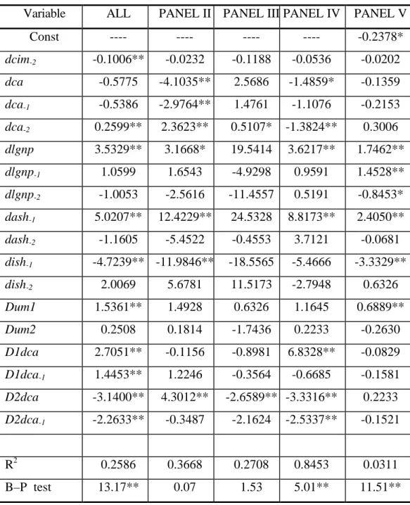
Including dummies does not change the results very much as shown in Table 4 (Panel II). The coefficient on D2dca reinforces the finding that donors with relatively high shares of aid experience increased imports by the recipient, suggesting that the effect of tying is positive and also has a magnitude less than one.18 The proportion of recipient imports from a particular donor does not appear to affect the aid-trade relationship (the Dum1
terms are insignificant). These results are consistent with Nilsson (1997) who finds that increased levels of tying do not necessarily generate increased trade with the recipient over and above that explained by control variables.
18 This can be seen by noting that for the sample for which the shares exceeds the threshold, D2 = 1, implying that the effect of the contemporaneous aid term on trade will be the sum of the coefficients on dCa and
Table 3 Aid to Trade Regressions (without Dummies) Dependent variable: Trade (volume change in imports)
Variable ALL PANEL II PANEL III PANEL IV PANEL V
Const ---- -0.3737 ---- -0.5988 -0.1251* dcim-2 -0.1365** 0.0040 -0.1808** -0.0079 -0.0130 dca 0.6903** -2.2674** 0.3160 5.0513** -0.0498 dca-1 0.2567** -2.7296** 0.4457 -1.7473** -0.3051 dca-2 0.1431* 2.5407** 0.3708 -1.5785** 0.3116 dlgnp 3.7111** 3.0924 24.2473 3.1042* 1.7524** dlgnp-1 0.8077 2.1908 -7.1746 0.6478 1.4597** dlgnp-2 -1.3865 -3.6953** -21.8486 -0.2872 -0.8706* dash-1 3.3047 10.7107** 28.7846 10.5049** 2.1317* dash-2 -0.4307 -7.1402** -8.4278 5.9148 -0.1982 dish-1 -4.3688* -10.1806** -22.0533 -9.4055** -3.2870** dish-2 1.8108 8.298** 30.0861 -4.0409 0.7699 R2 0.0999 0.2789 0.1039 0.7774 0.0340 B–P test 0.21 0.79 0.15 25.46 13.42** Wu-Hausman 99.34** 1.53 ---- 12.30 9.44 N.T 2626 286 182 546 1222 Estimator WG GLS WG GLS GLS
Notes: GLS estimates are reported if the Wu-Hausman test is rejected. WG estimators
are reported otherwise. The R2 is adjusted. B-P is the Breusch-Pagan test; N.T, the sample size is a product of the cross section and time series observations
respectively. t-statistics are suppressed; **, * indicate significance at the 5% and 10% levels respectively.
Table 4 Aid to Trade Regressions (with Dummies) Dependent Variable: Trade (volume change in imports)
Variable ALL PANEL II PANEL III PANEL IV PANEL V
Const ---- ---- ---- ---- -0.2378* dcim-2 -0.1006** -0.0232 -0.1188 -0.0536 -0.0202 dca -0.5775 -4.1035** 2.5686 -1.4859* -0.1359 dca-1 -0.5386 -2.9764** 1.4761 -1.1076 -0.2153 dca-2 0.2599** 2.3623** 0.5107* -1.3824** 0.3006 dlgnp 3.5329** 3.1668* 19.5414 3.6217** 1.7462** dlgnp-1 1.0599 1.6543 -4.9298 0.9591 1.4528** dlgnp-2 -1.0053 -2.5616 -11.4557 0.5191 -0.8453* dash-1 5.0207** 12.4229** 24.5328 8.8173** 2.4050** dash-2 -1.1605 -5.4522 -0.4553 3.7121 -0.0681 dish-1 -4.7239** -11.9846** -18.5565 -5.4666 -3.3329** dish-2 2.0069 5.6781 11.5173 -2.7948 0.6326 Dum1 1.5361** 1.4928 0.6326 1.1645 0.6889** Dum2 0.2508 0.1814 -1.7436 0.2233 -0.2630 D1dca 2.7051** -0.1156 -0.8981 6.8328** -0.0829 D1dca-1 1.4453** 1.2246 -0.3564 -0.6685 -0.1581 D2dca -3.1400** 4.3012** -2.6589** -3.3316** 0.2233 D2dca-1 -2.2633** -0.3487 -2.1624 -2.5337** -0.1521 R2 0.2586 0.3668 0.2708 0.8453 0.0311 B–P test 13.17** 0.07 1.53 5.01** 11.51**
Wu-Hausman 33.38** ---- ---- ---- 13.35
N.T 2626 286 182 546 1222
Estimator WG WG WG WG GLS
Notes: As for Table 3.
We now move to the question of whether there are any gains in pre-testing the data to identify separate panels. The results under ALL (Tables 3 and 4) form the basis of comparison. The Wu-Hausman test is rejected at the 5 per cent level of significance implying that the GLS estimates are inconsistent. The results reported are therefore the WG estimates that are still consistent even if the null under this test is rejected. Estimates from this sample show that all the aid terms in the equation are significant and positive. Added to this is the fact that they all have magnitudes that are consistent with what one will expect with the tying of aid.19 In particular the contemporaneous aid term has a magnitude of less than one, as expected if this term is capturing the proportion of tied aid. Looking at the lagged aid terms we notice that the magnitudes decline over time; again support for the tied aid story. We also note that per capita output growth has a positive net effect on trade in this equation.
Although only about 10 per cent of the total variation in the change in imports is being explained by the variables included, the results seem fairly consistent with an ‘aid engendering trade’ story using the ALL panel. When the dummies are included, the results appear even stronger. Imports seem to increase more from donors that are increasing their share of aid (positive coefficient on dash), but this is limited and the effect is negated if donors are already above the mean share of aid. Similarly, the ability to increase imports seems to decline over time: the effect of increasing import share on change in imports is negative, although it is positive for those donors with a high share of imports. Thus, the results for the ALL panel are consistent with the hypothesis that aid is an instrument of furthering trade objectives.
19 As already discussed output growth terms in the equation means the aid terms are only capturing the effect of tying on trade and not via output growth.
We demonstrate that this inference is misleading. Specifically, these coefficient estimates are averages over the entire sample whereas the other panels show that the coefficients vary significantly by sub-sample (i.e. the parameters are not common to all pairs). If aid leads to trade only for some donor-recipient pairs then it is inconsistent to proceed to estimate the relationship for all pairs in a combined sample. Indeed, in the specific sample where there is evidence for a causal effect of aid on trade, this effect is negative. The finding of a positive effect of aid on trade in the full sample is therefore a spurious result. If there is any justification in pre-testing the data and using that as a criterion for classification of panels, then we expect to find marked differences in the results across the panels. This is exactly what the results in Tables 2 and 3 portray.
First looking at the R2 statistics we observe that moving from the ALL sample to Panel II (which we argue is the appropriate sample for the study of the aid leading to trade hypothesis) increases our explanatory power from about 10 per cent to about 28 per cent. This is a marked increase given that the sample size of Panel II is much smaller. The R2 is highest for Panel IV (looking at both Tables 2 and 3). Most of the explanatory power here is coming from the contemporaneous aid term (leaving this term out reduces the R2 to about five per cent). Although the R2 is not the best criterion for model selection it is still indicative of the fact that the results obtained under the ALL sample are misleading.
Turning to the actual parameter estimates across the panels we observe significant differences from one panel to the other. In Panels II and III we get a negative net effect of aid on trade whereas in Panel IV it is positive. The magnitudes are also different compared with the ALL sample. An interesting observation here is that for Panel V aid has no effect on trade (i.e. neither in the Granger-sense nor in a contemporaneous way). This is consistent with the concept of Granger-causality that forms the basis of the categorisation of the panels. Although a finding of Granger-causality has a prima-facie element to it, a finding of ‘Granger non-causality’ is a much stronger result (Granger, 1988). This is a strong justification for the use of Granger-causality tests as the basis of classifying the donor-recipient pairs into the various panels. It reinforces the argument that it is not for every donor-recipient pair that one can find a relationship between aid and trade. These differences in results across panels don’t disappear with the introduction of the dummies.
Aid Allocation (Trade to Aid)
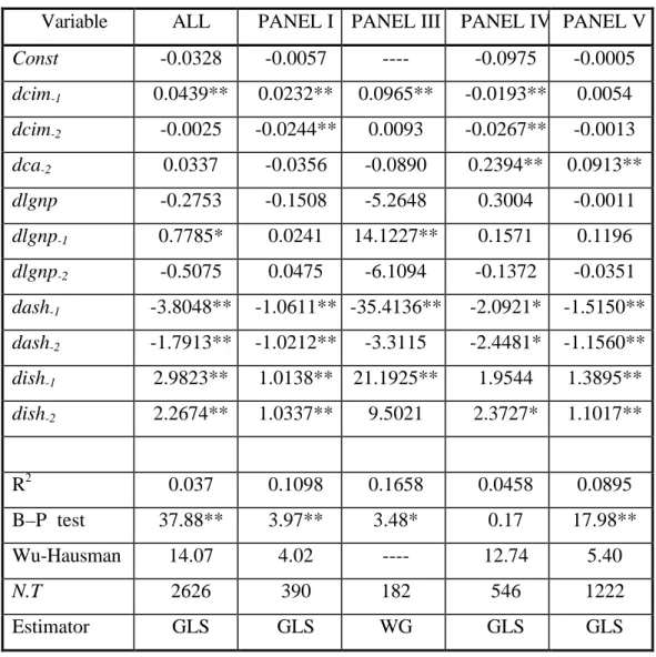
To analyse the effect of trade on aid we look at the Panel I estimates in Table 5 (sample of donor-recipient pairs for which trade is found to Granger-cause aid). Both the trade levels terms are significant with positive and negative signs for the one- and two-period lagged terms respectively. The net effect seems to be negative although it is insignificantly different from zero. In other words the level of trade does not seem to have a significant effect on aid. In the panel where trade appears to have a causal effect on aid, the net effect is zero when other variables are controlled for.
Table 5 Trade to Aid Regressions (without Dummies) Dependent Variable: Aid (change in volume)
Variable ALL PANEL I PANEL III PANEL IV PANEL V
Const -0.0328 -0.0057 ---- -0.0975 -0.0005 dcim-1 0.0439** 0.0232** 0.0965** -0.0193** 0.0054 dcim-2 -0.0025 -0.0244** 0.0093 -0.0267** -0.0013 dca-2 0.0337 -0.0356 -0.0890 0.2394** 0.0913** dlgnp -0.2753 -0.1508 -5.2648 0.3004 -0.0011 dlgnp-1 0.7785* 0.0241 14.1227** 0.1571 0.1196 dlgnp-2 -0.5075 0.0475 -6.1094 -0.1372 -0.0351 dash-1 -3.8048** -1.0611** -35.4136** -2.0921* -1.5150** dash-2 -1.7913** -1.0212** -3.3115 -2.4481* -1.1560** dish-1 2.9823** 1.0138** 21.1925** 1.9544 1.3895** dish-2 2.2674** 1.0337** 9.5021 2.3727* 1.1017** R2 0.037 0.1098 0.1658 0.0458 0.0895 B–P test 37.88** 3.97** 3.48* 0.17 17.98** Wu-Hausman 14.07 4.02 ---- 12.74 5.40 N.T 2626 390 182 546 1222 Estimator GLS GLS WG GLS GLS
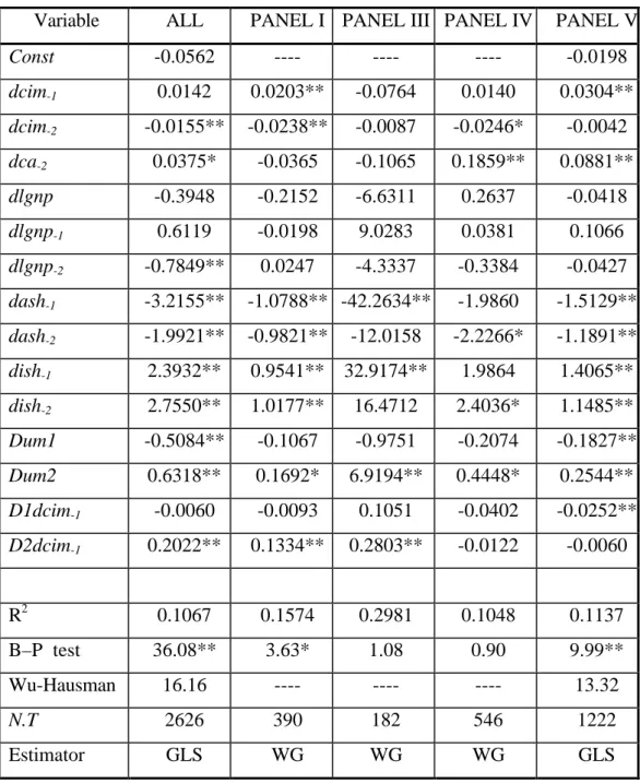
Table 6 Trade to Aid Regressions (with Dummies) Dependent Variable: Aid (change in volume)
Variable ALL PANEL I PANEL III PANEL IV PANEL V
Const -0.0562 ---- ---- ---- -0.0198 dcim-1 0.0142 0.0203** -0.0764 0.0140 0.0304** dcim-2 -0.0155** -0.0238** -0.0087 -0.0246* -0.0042 dca-2 0.0375* -0.0365 -0.1065 0.1859** 0.0881** dlgnp -0.3948 -0.2152 -6.6311 0.2637 -0.0418 dlgnp-1 0.6119 -0.0198 9.0283 0.0381 0.1066 dlgnp-2 -0.7849** 0.0247 -4.3337 -0.3384 -0.0427 dash-1 -3.2155** -1.0788** -42.2634** -1.9860 -1.5129** dash-2 -1.9921** -0.9821** -12.0158 -2.2266* -1.1891** dish-1 2.3932** 0.9541** 32.9174** 1.9864 1.4065** dish-2 2.7550** 1.0177** 16.4712 2.4036* 1.1485** Dum1 -0.5084** -0.1067 -0.9751 -0.2074 -0.1827** Dum2 0.6318** 0.1692* 6.9194** 0.4448* 0.2544** D1dcim-1 -0.0060 -0.0093 0.1051 -0.0402 -0.0252** D2dcim-1 0.2022** 0.1334** 0.2803** -0.0122 -0.0060 R2 0.1067 0.1574 0.2981 0.1048 0.1137 B–P test 36.08** 3.63* 1.08 0.90 9.99** Wu-Hausman 16.16 ---- ---- ---- 13.32 N.T 2626 390 182 546 1222 Estimator GLS WG WG WG GLS
Notes: As for Table 3.
The other significant variables in the regression are the aid share and trade share terms with negative and positive net effects respectively. If the share of aid adequately captures the political ties between any donor-recipient pair then our results suggest that political
ties (as well as colonial ties) are not too important in aid allocation decisions.20 Such ties may establish initial levels of aid, but over time aid flows tend to increase less for those donors contributing a greater share of recipient aid. The positive effect of the import share terms can be interpreted as reflecting the significance of the strategic importance of a recipient in aid allocation decisions of donors. Donors do appear to give more aid to recipients that buy proportionately more imports from the donor. Note that, when other variables are controlled for, GNP growth does not appear to have an effect on the change in aid flows, i.e. recipient needs is not a determinant of bilateral aid flows (when both are evaluated as changes).
Including the dummies does not alter the results Panel I significantly, although explanatory power is increased (Table 6). The coefficients on Dum2 and the multiplicative import share with aid dummy are both significant and positive. When a recipient increases imports from a donor (conditional on it having above average aid from that donor), they are rewarded with more aid. This is additional to the tendency of donors with an above average share of aid to the recipient to increase aid by more than other donors. These findings are tentative for the reason discussed in section 4 (see footnote 20). They are suggestive of the fact that the share of imports is as important as its level in aid allocation decisions of donors; a result consistent with McGillivray and Oczkowski (1991).
We now turn to the question of whether there are any differences in the results under the different panels. Consider the estimates obtained when the sample of all donor-recipient pairs is used. For this sample we cannot reject the Wu-Hausman test and so GLS estimates are reported. The net trade effect on aid is positive (although appears to be offset when the dummies are included). This is also the case for the net effect of per capita output growth on aid. All the aid and trade share terms are also significant. On the face of it, the results appear to support the standard aid allocation argument. Aid from a donor increases more if the share of imports from that donor increases (especially if the donor gives an above average share of aid), although this effect is reduced if the donor has an above average share of imports. It is evident that it is import and aid shares, not their
20 As the decision (or dependent) variable is ‘donor-centred’ a better proxy for political ties will be the share of the donor’s total aid that goes to the recipient. as opposed to the share of a donor’s aid in a recipient’s total
level, that appear to determine changes in aid volumes. Donors appear to be influenced by relative considerations rather than absolute ones.
Although over half of the regressors are individually significant for the ALL sample, they explain only about four per cent of the total variation in the changes in aid (ten per cent when dummies are included). One reason could be that we have omitted some important variables that help explain allocated aid; this is certainly true to some extent. On the other hand, the low explanatory power can be interpreted to mean that the results are spurious. The fact that the dependent variable is aid disbursements rather than commitments could partly explain why we get this very low explanatory power (but cannot be all of the explanation). This, however, will be true for all the different panels considered.
A plausible inference is that it is the pooling that gives rise to potentially spurious results. Comparing estimates across the different panels we make the following observations. First, under Panel V we find that the level of trade does not have any effect on aid (import shares remain significant). This reaffirms the earlier point made about Granger-causality tests (i.e. a finding of Granger non-causality is a much stronger result). Second, the net effect of trade on aid in the equation is different for the different samples. Under Panel I we observe that trade has a zero net effect on aid. For Panels III and IV the net effects are respectively positive and negative. Aid and trade shares have respectively negative and positive net effects for all the panels, although the coefficient estimates and significance levels vary considerably.
The pattern of the results doesn’t change very much when dummies are introduced (Table 6). For instance the R2 remains highest for Panels I and III, about 16 per cent and 30 per cent respectively. These results suggest a very simple but oft-neglected fact: a large sample is not necessarily the best sample. Although there is the same number of significant variables in the equation, the R2 increases from about ten per cent under ALL to about 16 per cent for Panel I. A more appropriate sample performs better than the large sample. While the broad inferences are the same comparing ALL and Panel I (more so than in the case of the aid to trade relation). In particular, GNP growth appears on balance to have
used here. The latter is more appropriate for the aid to trade analysis in which the dependent variable is ‘recipient-centred’.
the expected negative impact on aid in the ALL sample (when dummies included), but is not significant in Panel I. Similarly, the level of imports appears to have a small net positive impact for ALL, but is not significant for Panel I. For those donor-recipient pairs where there is evidence of a causal effect of trade on aid, our evidence suggests that this is due primarily to import shares. When we consider all pairs, other factors play a role but the overall explanatory power is reduced.
VI. CONCLUSIONS
Our aim here is not to judge which panel best fits our expectations in terms of explaining any relationship between aid and trade. We are not actually testing between alternative explanations or models. However, the specifications we estimate are representative of the literature, and we have shown that if one uses a panel comprising all observations, the results are broadly in line with those in the literature. Our main argument is that such results are misleading if not spurious. If the nature of the time series relationship underlying specific observations differs, these should not be pooled into one panel. Specifically, if there are differences in the bivariate causal relationship for the variables of concern (aid and trade flows for donor-recipient pairs in our example), separate panels should be identified. Our results show that there can be significant differences between the results for distinct panels, especially if compared to the results from a panel comprising all observations.
The paper investigated some of the issues that the empirical analysis of the aid and trade relationship raises, with a view to testing the validity of pooling countries in large panels. We began with a set of observations on bilateral aid and trade flows between four donors and 26 African recipients (a potential set of 104 pairs, although there were no observations for some) over 1969-95. Given lagged variables and missing data, the total sample comprised 2626 observations. Based on results from bivariate Granger-causality tests of aid and trade for all pairs over time, we formed five sub-panels. For the analysis of the aid to trade hypothesis we used results from Panel II, the sample of donor-recipient pairs for which aid is found to Granger-cause trade. Panel I, the sample of donor-recipient pairs for which trade is found to Granger-cause aid is used to analyse the issue of aid allocation decision of donors (i.e. the trade to aid hypothesis). We compared the results from the sub-panels with those obtained when all observations are pooled. Appropriate panels can yield unexpected results. For example, in the panel where aid caused trade, the
levels effect was negative; the positive effect arose through share variables. The main result is that pooling matters, and gives rise to misleading results. Identifying appropriate panels provides more meaningful results. There were a number of findings specific to the nature of the relationship between aid and trade.
We find little support for the hypothesis that the tying of aid generates trade over and above that explained by control variables, a result consistent with the findings of Nilsson (1997). For the panel where aid had a causal effect on trade, the effect of the change in the level of aid on the change in the level of imports was negative. For this panel, GNP growth was not a significant determinant of imports, but donor aid shares had a significant positive effect. Thus, where aid causes trade, aid shares (donor-recipient ties) rather than changes in volumes (formal tying) appear to be the dominant effect. Accepting the results from pooling all observations would lead to different conclusions. In particular, one would be lead to conclude that higher aid volumes (tied aid) do increase trade, whereas aid shares have a weak if any effect. In these regressions, GNP growth has a significant positive effect on trade growth. However, aid does not cause trade for the full sample (only for the sub-sample) and these inferences are incorrect. A more plausible inference for the entire sample is that there is a tendency for imports to increase with growth, and there has also been a tendency for aid to increase in a way that is weakly correlated with growth (recall that the recipients are all African). Hence a pooled regression reveals a positive correlation between aid and trade. To infer from this that aid increases trade is wrong, as the result is spurious.
In the case of aid allocation (the trade to aid relationship), our results suggest that the share of imports is the important factor in the aid allocation decision of donors. This is a finding in the panel for which there is evidence of a causal effect of trade on aid, and for a regression using the entire sample. This could therefore be described as a robust finding. In fact, for aid allocation the findings for the full panel and ‘causal’ panel are quite similar. However, for those pairs where trade causes aid, there is no evidence that the level of imports determines the level of aid, nor that GNP growth affects changes in aid. When trade causes aid, it is import shares that really matter. For the full sample other factors also matter, there is a weak positive effect of the import level and a weak negative effect of GNP growth. Identifying appropriate panels does provide new information, even if only to qualify rather than alter the finds from the full pooled sample.
The most important finding is it is inappropriate to do an empirical analysis of the aid and trade relationship without pre-testing the data, to identify sub-panels according to the underlying direction of causality. In other words large samples are not necessarily the best
samples. This result casts doubt on the general validity of the findings in empirical macroeconomic studies that use pooled panel data. It is not simply a case that cross-section heterogeneity matters. This is well known and can be addressed, for example through fixed or random effect estimators (although not all studies test this carefully). The additional point we make is that there can be time series heterogeneity. This arises if there is an implicit causal relationship that may differ for countries in the sample. We tested for causality between aid and trade flows. When sub-panels were constructed according to the evidence from bivariate causality tests and then used in a more general model with control variables, it did make a difference. This may have applications for other macroeconomic relationships where causality can be in either direction, for example aid and growth, investment and growth or exports and growth. This may be one reason why the results from empirical growth studies have been so inconclusive and disappointing.
REFERENCES
Bahmani-Oskooee, M. and A. Nasir (2001), ‘Panel Data and Productivity Bias Hypothesis’, Economic Development and Cultural Change, 49:2, 395-402.
Baltagi, B. H. (1995), Econometric Analysis of Panel Data, John Wiley and Sons Ltd., West Sussex.
Benassy, Jean-Pascal, (1986), Macroeconomics: An introduction to the Non-Walrasian
Approach, Academic Press, London.
Borensztein, E., J. de Gregorio and J-W. Lee (1998), ‘How does foreign direct investment affect economic growth’, Journal of International Economics, 45, 115-135.
Bruesch, T and Pagan, A (1979), ‘A Simple Test for Heteroscedasticity and Random Coefficient Variation’, Econometrica, 47, 1287-1294.
Burnside, C. and D. Dollar (2000). ‘Aid, Policies, and Growth.’ American Economic
Review, 90:4, 847-868.
Chang, J. Y. and R. Ram (2000), ‘Level of development, rate of economic growth and income inequality’, Economic Development and Cultural Change, 48:4, 787-799. Cnossen, T., M. McGillivray, and O. Morrissey (1999), ‘Is there a link between Aid and
Trade Flows? An Econometric Investigation’ in K. Gupta (ed), Foreign Aid: New
Perspectives, Boston MA: Kluwer Academic Publishers.
Granger, C. W. J. (1988), ‘Some Recent Developments in a Concept of Causality’,
Journal of Econometrics, 31, 199-211
Greene, W. H. (1997), Econometric Analysis, Third Edition, Prentice-Hall International, New Jersey.
Hansen, H. and F. Tarp (2001), ‘Aid and Growth Regressions’, Journal of Development
Economics, 64:2, 547-570.
Hausman, J. A. (1978), ‘Specification Tests in Econometrics’, Econometrica, 46:6, 1251-1272
Hsiao, C. (1986), Analysis of Panel Data, Cambridge: Cambridge University Press. Jepma, C. (1989), ‘The Tying of Aid’, University of Groningen: International Foundation
for Development Economics.
Kenny, C. and D. Williams (2001), ‘What do we know about Economic Growth? Or why don’t we know very much?’, World Development, 29:1, 1-22.
Lloyd, T., M. McGillivray, O. Morrissey and R. Osei (1998), ‘Investigating the Relationship between Aid and Trade Flows, CREDIT Research Paper 98/10,