Round-Robin Routing Policy
Value Functions and Mean Performance with Job- and Server-specific Costs
Esa Hyytiä
Department of Communications and Networking Aalto University, Finland
Samuli Aalto
Department of Communications and Networking Aalto University, Finland
[email protected]
ABSTRACT
We study the Round-Robin (RR) routing to a system of par-allel queues. The cost structure comprises two components: a service fee and a queueing delay related component, where both can be job- and queue-specific random variables. With Poisson arrivals, the inter-arrival time to each queue obeys Erlang’s distribution. This allows us to study the mean and transient behavior of the queues separately. The service fee is independent of the queueing, and we obtain the corre-sponding mean cost rate and value function in closed forms. With respect to queueing delay, we first derive integral ex-pressions enabling efficient computation of the correspond-ing value function. By decomposition, these yield also the value function for the whole system of m parallel queues fed by RR. Given the value function, one can carry out the first policy iteration step with arbitrary holding cost rates (e.g., delay, slowdown etc.) yielding efficient size-, cost- and state-aware policies. Moreover, the mean waiting time in an M/G/m-RR system gets resolved at the same time. The re-sults are demonstrated in the numerical examples, where we compute near optimal task assignment policies for a sample system with two servers.
Keywords
Round-Robin, M/G/m-RR, Erl/G/1 queue, Task assign-ment, Dispatching, Parallel queues, MDP
1.
INTRODUCTION
In the task assignment (or routing) problems, one chooses a server for each new job immediately upon the arrival. The objective is to minimize the mean response time, slowdown, energy consumption, or some other performance quantity of interest. Within each queue, theFirst-Come-First-Served
(FCFS) scheduling is usually assumed, but other scheduling disciplines can also be considered. Even though task assign-ment problems have been studied extensively in the liter-ature, only a few optimality results are known, and these generally require homogeneous servers.
Permission to make digital or hard copies of all or part of this work for personal or classroom use is granted without fee provided that copies are not made or distributed for profit or commercial advantage and that copies bear this notice and the full citation on the first page. To copy otherwise, to republish, to post on servers or to redistribute to lists, requires prior specific permission and/or a fee.
ValueTools’13,December 10 – 12 2013, Turin, Italy Copyright 2013 ACM 978-1-4503-2539-4/13/12 ...$15.00.
TheJoin-the-Shortest-Queue (JSQ) policy assigns a new job to the server with the fewest tasks. Assuming exponen-tially distributed inter-arrival times and job sizes, and ho-mogeneous servers, [33] showed that JSQ, followed by FCFS, minimizes the mean delay. Since then the optimality of JSQ has been shown in many other settings [32, 9, 18, 31, 29, 24, 1]. Similarly, Round-Robin (RR), followed by FCFS, has been shown to be the optimal policy when it is only known that the queues were initially in the same state, and the routing history is available [9, 27, 26]. For RR com-bined with the Shortest-Remaining-Process-Time (SRPT) scheduling, see [8]. With a Poisson arrival process and RR, the inter-arrival times to each queue obey Erl(m, λ) distri-bution, wheremdenotes the number of servers [15].
TheLeast-Work-Left (LWL) policy assigns a new job to the queue with the least amount of unfinished work. LWL is equivalent to M/G/m with a shared queue [16, 15], and thus it makes sure no server is idle when there are jobs in the queue. Interestingly, with constant service times, LWL, JSQ and RR make equivalent decisions as in M/D/m(with a shared queue), which can also be shown to be optimal with respect to the mean delay.
The M/G/msystem is non-trivial to analyze. More re-sults are available for M/D/m. The first analytical result for the distribution of waiting time in M/D/mis by Crommelin [6]. Numerically much more stable expressions are given by Franx [11], who has also analyzed its transient behavior in [12]. In particular, [11] gives the waiting time distribution as a function of the queue length distribution, allowing also the determination of the mean waiting and sojourn times. For extensive surveys on the topic we refer to [30, 23].
Value functions for single server queues withPoisson ar-rivalshave been derived in [25, 2, 5, 21], which form the basis also for value functions for task assignment systems operat-ing under a state-independent policy such as the Bernoulli-split. With state-dependent policies, such as RR and LWL, the queues are coupled and the analysis gets more compli-cated. In this paper, we derive a set of integral equations that enable efficient computation of the value function with respect to arbitrary holding cost based cost structure in a size-aware task assignment system subject to RR routing policy and FCFS scheduling discipline. Jobs arrive accord-ing to a Poisson process with rate λ and the servers are assumed to be identical.1 As an interesting and useful side
1In fact, the analysis does not depend on this and the results
hold with very minor modifications also for heterogeneous systems. However, the Round-Robin policy is not an ideal candidate if the service rates are highly asymmetric.
Round Robin
FCFS
λ
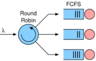
Figure 1: Round-Robin routing to m servers.
product, these expressions also provide a new approach to determine the mean waiting time in an M/G/m-RR system, whereas using the results given in [11] for M/D/m-RR re-quires the determination of the queue length distribution as an intermediate result.
The rest of the paper is organized as follows. First, in Sec-tion 2, we analyze a single Erl/G/1 queue and derive both differential and integral expressions for the value function. Due to the decomposition, the value function for M/G/m -RR is also obtained. Section 3 discusses the task assignment problem and policy iteration, and gives some numerical ex-amples. Section 4 sheds light on possible more elaborate applications, and Section 5 concludes the paper.
2.
ANALYSIS OF THE ROUND-ROBIN
In this section, we analyze the Round-Robin routing pol-icy illustrated in Fig. 1. With Poisson arrivals, the arrival process to each queue is Erl(m, λ)/G/1, which facilitates the analysis. First we describe the model and the cost structure, and then derive expressions for calculating the value func-tions for arbitrary job- and queue-specific service fees and holding cost rates, which also give the mean delay.
2.1
Model and Cost Structure
We consider a stable M/G/m-RR system illustrated in Fig. 1. With a Poisson arrival process, each queue behaves according to an Erl(m, λ)/G/1 queue, where the inter-arrival time in each queue is a sum ofm independent and expo-nentially distributed time-intervals, i.e., phases, with mean durations of 1/λ. Jobs arrive at the end of phase m, after which a new phase 1 starts. The evolution of the queues is naturally coupled as they see the same Poisson process, while each of them is in a different phase (1, . . . , m). The cost structure comprises two components. First, Jobjpays aservice feeofSjupon entering a queue. Second, it incurs
costs atholding cost rate Hj while waiting in a queue.2
We further assume that the service time X, the service feeS and the holding cost rate H all may depend on the queue a job is assigned to. Thus, in general, Job j is de-fined by triples (Xj,k, Hj,k, Sj,k), where k corresponds to
the queue,k= 1, . . . , m. In practice, the holding cost rate is often job-specific, Hj,k = Hj and the service fee is
ei-ther a server-specific constant or a function of service time, Sj,k=gk(Xj,k) (e.g., per bit charging in mobile networks).
That is, one can associate the holding cost with the queueing delay a job experiences and the service fee with a (server-specific) service cost/time (e.g., energy). In particular, we assume that jobs are i.i.d.,
(Xj,Hj,Sj)∼(X,H,S),
2
This is slightly different than, e.g., in [20, 22], where the holding costs are incurred also during the service time. In our case, an equivalent cost can be defined using service fees.
while the different variables of a single job may depend on each other (e.g., the service fee can be equal to the service time). Note that withH= 1 andS=X, the costs incurred are equal to the sojourn time.
With RR, the jobs are assigned sequentially, indepen-dently of their holding cost rates and service fees, and hence the above cost structure is unnecessarily complicated. How-ever, later in Section 3, we consider also routing policies that take into account the job- and server-specific characteristics, and hence the notation.
2.2
State description for Round-Robin
When all servers are identical, the service fees can be omitted and the state of the Round-Robin system can be described by anm-tuple,
z= (u1, . . . , um),
whereuidenotes the backlog in the queue currently in phase
i. Similarly, when considering the service fees, only the phase matters and a sufficient state description is
z= (q1, . . . , qm),
where qi is the index of the queue currently in phasei. In
general, the state of the system can be described by
z= ((q1, u1), . . . ,(qm, um)),
where (qi, ui) denotes the server and its backlog that is
cur-rently in phasei. Therefore, (q1, . . . , qm) is some
permuta-tion of (1, . . . , m), whereasui≥0 for alli.
2.3
Service Fees
Let us first consider the service fees each Erl/G/1 queue incurs. Let Sj ∼ S denote the service fee of the jth job
assigned to a given queue. Then let i denote the current phase in the arrival process, i= 1, . . . , m, such that at the end of phasema job arrives and a cost ofSjis incurred.
A sufficient state description with respect to service fees is the current phase of the arrival process. Consequently, the correspondingvalue function depends also only on the current phase, and it is defined as the expected difference between a system initially in phaseiand a system initially in equilibrium,
vi, lim
t→∞E[Vi(t)−rst], (1)
where Vi(t) denotes the service fees incurred during (0, t)
when initially in phase i, and rs is the mean rate at which
service fees are incurred,
rs=
λE[S] m .
Proposition 1. The value function with respect to
ser-vice fees for an Erl(m, λ)/G/1 queue is
vi=
2i−m−1
2m E[S]. (2)
whereidenotes the current phase of the arrival process,i= 1, . . . , m, andE[S]is the mean service fee.
Proof. Value function, as defined in (1), measures the expected difference in the cumulative costs from the given initial phaseito the mean cost rate. For an arbitrary phase i, the so-called Howard’s equation is
vi=
m−i+ 1
The first term corresponds to the time interval before the next arrival. During this time no service fees are collected and the difference to the mean cost rate is 0−rs. The factor
(m−i+ 1)/λcorresponds to the mean time duration. The second term is the mean immediate cost due to the following arrival, after which the arrival process enters to phase 1. The mean difference in costs between phase 1 and the mean cost rate isv1 by definition, i.e.,v1 takes care of
the future costs from that point onwards (recall the Markov property). Consequently,
vi−v1=
i−1
m E[S]. (3)
As each phase is equally likely, we haveP
ivi= 0. Taking
a sum of (3) overigivesv1, which in turn yields (2).
Consider next the whole M/G/m-RR system and letS(k) denote the service fee in Queuek. Due to the decomposition, we have the following result:
Corollary 1. The value function w.r.t. service fees for
the M/G/m-RR system in statez= (q1, . . . , qm)is
v(z) = 1 2m m X i=1 (2i−m−1)E[S(qi)]. (4)
Note that the value function is insensitive to the arrival rate λand depends only on the phases (i.e., the RR sequence) and the mean service fees. In fact, the constant offset in the value functions is irrelevant to us, and we can equally use
v(z) = 1 m m X i=1 iE[S(qi)], (5)
from which it is obvious that the Round-Robin sequence assigning the jobs (initially) in the increasing order of the mean service fee so that E[S(qi)]≤E[S(qi+1)] incurs the least
costs, as expected.
2.4
Virtual Waiting Time
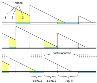
We are often interested in the mean waiting and sojourn time in a system. To this end, we define thevirtual waiting time in the system as the backlog of the queue receiving the next customer. More precisely, we define the holding cost rate of the system to be equal to the backlog of the queue in phasem. Considering an individual Erl(m, λ)/G/1 queue, it thus incurs costs at the rate equal to the backlog only during phasem, at the end of which a new job arrives. This is illustrated in Fig. 2. Due to the PASTA property, this corresponds to the waiting time the jobs arriving to the M/G/m-RR system see. Let ˜rdenote the mean cost rate in a single queue andr in the whole system,r= E[W]. With identical servers, we have the elementary relationship
˜ r=r/m.
In general, the service times may be heterogeneous and
r= E[W] = (1/m)P kE[W (k) ] r=P kr˜ (k) ⇒E[W (k) ] =mr˜(k).
2.4.1
Single Erl/G/1 Queue
Consider next a single Erl(m, λ)/G/1 queue and letF(x) denote the cdf of the service timeX. LetIt(i) andUt(i, u)
denote the phase of the arrival process and the backlog in the queue at time t, where (i, u) denote the initial phase,
(λ)
Exp Exp(λ) Exp(λ)
costs incurred phase
1 2 3
Figure 2: Sample path with m=3 queues.
i= 1, . . . , m, and the initial backlog,U0(i, u) =u. In this
RR-specific cost structure, the queue incurs costs at rate Ct(i, u),1(It(i) =m)·Ut(i, u).
Let vi(u) denote the value function, where i is the initial
phase anduthe initial backlog. Formally, vi(u), lim
t→∞E[Vi(u, t)−˜r t],
where Vi(u, t) denotes the costs a queue initially in state
(i, u) incurs during timet,
Vi(u, t), Z t
0
Cs(i, u)ds.
Proposition 2. The value function of an Erl(m, λ)/G/1 queue with respect to the virtual waiting time satisfies the following system of integro-differential equations,
v0i(u) =−˜r+λ(vi+1(u)−vi(u)), i= 1, .., m−1 v0m(u) =u−˜r+λ ∞ Z 0 (v1(u+s)−vm(u))dF(s). (6)
Proof. For u > 0, small δ > 0, and for phases i = 1, . . . , m−1
vi(u) = (0−˜r)δ+(1−λδ)vi(u−δ)+λδ vi+1(u−δ).
The first term corresponds to the difference between the cur-rent cost rate (zero for phasesi6=m) and the mean cost rate ˜
rmultiplied by the time-intervalδ. With the probability of (1−λδ), the phase remains the same andvi(u−δ) gives the
future contribution, and with the probability ofλδ, the ar-rival process moves to the next phase i+ 1, the value of which is given byvi+1(u−δ). In contrast, at the end of last
phasema new job arrives, and thus for vm(u) we have
vm(u) = (u−˜r)δ+(1−λδ)vm(u−δ)+λδ ∞ Z
0
v1(u+s)dF(s).
Asδ→0, the above yields (6).
For the special case of a constant service time ∆, the latter equation in (6) reads
and we have a first-order system of differential equations. Considering an empty system withu= 0 gives
˜ r =λ(vi+1(0)−vi(0)), i= 1, . . . , m−1, ˜ r =λ ∞ R 0 (v1(s)−vm(0))dF(s). (7)
With a constant service time ∆, the latter equation reads ˜
r=λ(v1(∆)−vm(0)).
Combining (6) and (7) gives,
v0i(0) = 0, i= 1, . . . , m,
v00i(0) = 0, i= 1, . . . , m−1.
(8)
Adding the equations (7) together gives
mr˜=r=λ
Z ∞
0
(v1(s)−v1(0))dF(s), (9)
which for a constant service time ∆ reduces to mr˜=λ(v1(∆)−v1(0)).
Similarly, we have for alli= 1, . . . , m−1
vi+1(0)−v1(0) =
i˜r
λ. (10)
That is, initially the value functionsvi(u) atu= 0 differ by
a constant amount of ˜r/λ.
Note that both (6) and (7) are insensitive to a constant term in thevi(u). The constant offset in the value
func-tions indeed is generally superfluous and we can set, e.g., v1(0) = 0. Unfortunately, (6) and (7) are difficult to solve
even numerically. If the mean cost rate ˜r was available in a closed form, (7) would give the initial values vi(0) = 0
also fori = 2, . . . , m. Moreover, even if the initial values were available,vm0 (u) still depends on thev1(u+s),s >0,
and therefore the standard Runge-Kutta method could not be applied to compute the vi(u) foru > 0. However, one
could solve thevi(u) numerically backwards foru < u∗given
thevi(u∗) were available for someu∗ >0. We describe an
elegant approach to solve thevi(u) and ˜r in Section 2.4.4.
Finally, withm= 1 the Erl/G/1 queue reduces to M/G/1, for which the exact value function is available [21]
v(u)−v(0) = u
2
2(1−ρ). (11) It is easy to see that (11) satisfies (6), and applying to (7) gives, as expected, the Pollazcek-Khinchine formula for the mean waiting time.
2.4.2
M/G/
m-RR System
Consider next the whole M/G/m-RR system. In general case, the servers may be heterogeneous and the value func-tions have to be determined separately for each of them. Letv(ik)(u) denote the value function of Queuek currently in phasei. Due to the decomposition tomparallel Erl/G/1 queues, we again have:
Corollary 2. The value function w.r.t. virtual waiting time for M/G/m-RR in statez= ((q1, u1), . . . ,(qm, um))is
v(z) =v(1q1)(u1) +. . .+vm(qm)(um). (12)
If the service timesXj,kare identical for every queuek, then
v(z) =v1(u1) +. . .+vm(um).
2.4.3
Asymptotic Behavior
Below we argue that, with relatively broad assumptions, the asymptotic behavior of the value function of the G/G/1-FCFS queue is quadratic. For largeu, the backlog decreases with an average rate of 1−ρ0, where ρ0 denotes the queue specific offered load. The virtual waiting time incurred dur-ing the remaindur-ing busy period corresponds to a triangle with initial heightuand base (= duration)u/(1−ρ0). Therefore,
v(u)≈ u
2
2(1−ρ0)−
u
1−ρ0 ·r+v(0),
where the first term corresponds to the costs incurred during the remaining busy period, the second term to the mean cost rate during the same time-interval, and the third term corresponds to what happens after that. For large u, the first quadratic term dominates.
With Erl(m, λ)/G/1, in the context of RR, the costs are accrued only in the final phase m as explained above (see also Fig. 2). Let ρ denote the offered load to the whole system, ρ=λE[X], so thatρ0 =ρ/m. The costs accrued during the remaining busy period are roughly 1/m of the “full triangle”, i.e., foru1 we have,
vi(u)≈ u2 2(m−ρ), and v 0 i(u)≈ u m−ρ. (13)
2.4.4
Numerical Solution for
vi(u)The equations (6) that the value functionsvi(u) must
sat-isfy can be written in an integral form that is suitable for numerical computations:
Proposition 3. For an Erl(m, λ)/G/1 queue, the value functionvi(u)with respect to the virtual waiting time satis-fies the following system of integral equations,
vi(u) = e−λu−1 i vi+1(0) +λ u Z 0 e−λ(u−s)vi+1(s)ds, i= 1, . . . , m−1, vm(u) = e−λu−1 m Z∞ 0 v1(s)dF(s) +e −λu+λu−1 λ2 +λ u Z 0 e−λ(u−s) ∞ Z 0 v1(s+`)dF(`)ds. (14)
Proof. For i= 1, . . . , m−1, multiplying both sides of (6) witheλu gives
eλuv0i(u) +λe λu
vi(u) =eλu(−˜r+λvi+1(u)).
The left-hand side is equal to (d/du)eλuvi(u), yielding
eλuvi(u) = u Z 0 eλs(−r˜+λvi+1(s))ds+vi(0), vi(u) = ˜ r λ(e −λu −1) +e−λuvi(0) +λ u Z 0 e−λ(u−s)vi+1(s)ds.
Similarly, for phasemone obtains
vm(u) = ˜ r λ(e −λu −1) +e−λuvm(0) + e−λu+λu−1 λ2 + λ Z u 0 e−λ(u−s) Z ∞ 0 v1(s+`)dF(`)ds.
As we are generally interested in the differences between the relative values, we can setv1(0) = 0 so that
vi(0) = (i−1)˜r λ , fori= 1, . . . , m, and ˜ r λ = vi+1(0) i , fori= 1, . . . , m−1, 1 m Z∞ 0 v1(s)dF(s).
Substituting these into the above gives (14).
Corollary 3. For a constant service time∆, the latter equation in (14)reads vm(u) = e−λu− 1 m v1(∆) + e−λu+λu−1 λ2 +λ u Z 0 e−λ(u−s)v1(s+ ∆)ds. (15)
Note that (14) expresses vi(u) as a function vi+1(u) for
i= 1, . . . , m−1, andvm(u) as a function ofv1(u). Given an
initial guess for anyvi(u), provided, e.g., by (13), the
equa-tions (14) can be iterated until they converge. In practice, the convergence turns out to be fast.
As a convenient side product of being able to determine the value functions efficiently, also themean waiting time, r= E[W], is obtained (withv1(0) = 0):
Corollary 4. Solving the value functions using(14)gives also the mean waiting timeE[W]in the system,
E[W] =λ m v2(0), (16)
In order to compute E[W], we do not need to find the waiting time distribution first (which itself is non-trivial, [11]).
Form= 1, the insensitive solution (11) can be shown to satisfy (14). That is, for the M/G/1 queue we have,
v(u) =e−λu−1 ∞ Z 0 v(s)dF(s) +e −λu +λu−1 λ2 +λ u Z 0 e−λ(u−s) ∞ Z 0 v(s+`)dF(`)ds, which “trial” v(u) = u 2 2(1−ρ),
satisfies independently of the service time distribution.
2.4.5
Generalized Round-Robin (GRR)
RR is a special case of theGeneralized Round-Robin poli-cies defined by predefined typically periodic sequences [13, 14, 3]. RR is optimal under certain assumptions when the servers are identical. However, if some servers have different service rates, then the even split of tasks that RR carries out may no longer make sense. In [13], Hajek proves the intuitive result that among a very large class of arrival pro-cess, the one with constant inter-arrival times is optimal for a single server queue with exponentially distributed ser-vice times. Then, in [14], he shows that the so-called most-regular-sequence is optimal for two, not necessarily identical, servers when jobs again obey exponential distribution.
Suppose that the (external) sequenceaidefining the task
assignments is periodic with m denoting the length of the period. Without lack of generality, we can consider Queue 1. With respect to service fees, both the mean rate and value function are straightforward to deduce. We omit these for brevity. For the virtual waiting time, letvi(u) again denote
its value function with respect to the backlog (in phases with actual arrivals, ai = 1). For notational convenience,
we define vi+m(u) ,vi(u). Similarly as earlier, we have a
system of differential equations,
v0i(u) = −r˜+λ(vi+1(u)−vi(u)), ifai6= 1, u−˜r+λ Z (vi+1(u+t)−vi(u))dF(t), ifai= 1,
where the initial values are coupled,
v0i(0) = −r˜ λ+vi+1(0), ifai6= 1, −r˜ λ+ Z vi+1(t)dF(t), ifai= 1.
That is, the generalized (periodic) RR can be analyzed es-sentially the same way as RR. Also probabilistic variants, where subsequences are chosen with certain probabilities (for load-balancing reasons), are amenable to the same approach.
2.5
Waiting Time and General Holding Costs
Consider next M/G/m-RR with identical servers. The backlog based holding cost ratec(z) =um can be seen as a
penalty for a long queue length. However, often one is in-terested in the actualwaiting time, possibly weighted with arbitrary job-specific holding costs. Let U(t) =Um(t)
de-note the virtual waiting time at timet. With FCFS, this is the waiting time an arriving customer sees, W ∼U. The mean cost rate w.r.t. waiting time is
rW =λ·r=λ·E[W],
i.e., the rate at which the system incurs waiting time.
Proposition 4. The value function for an M/G/m-RR system with respect to waiting time is
˜
v(z) =λ v(z) (17)
wherev(z)is the value function w.r.t. virtual waiting time.
Proof. LetW1, W2, . . .denote the waiting times related
to the future arrivals. One can associate the costs in two equivalent ways for these arrivals until the end of the current busy period (renewal point),
˜ c1 ,λE[ Z Bz 0 Um(t)dt], ˜ c2 ,E[W1+. . .+WNz], (18)
whereBzdenotes the duration of the (remaining) busy
pe-riod (having a finite mean), andNzthe number of jobs
ar-riving during it. Due to the PASTA property, ˜c1= ˜c2. The
first equation corresponds to the virtual waiting time based holding costc(z) =ummultiplied by the arrival rateλ, and
the latter to the actually incurred waiting time. Then, ˜ v(z)−˜v(0) = E[W1+. . .+WNz]−rWE[Bz] =λE[ ZBz 0 (Um(t)−r)dt] =λ(v(z)−v(0)),
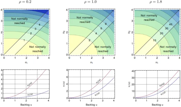
ρ= 0.2 ρ= 1.0 ρ= 1.8 v1HuL v2Hu L 0 1 2 3 4 0 1 2 3 4 5 6 Backlog u vi H u L v1Hu L v2Hu L 0 1 2 3 4 0 2 4 6 8 Backlog u vi H u L v1Hu L v2Hu L 0 1 2 3 4 0 10 20 30 40 Backlog u vi H u L
Figure 4: Value function for M/D/2-RR with respect to the virtual waiting time.
Waiting time Sojourn time MD1 MD2 MD1 MD2 0 0.2 0.4 0.6 0.8 1 1.2 1.4 0 0.5 1 1.5 Arrival rateΛ M e a n ti m e
Mean waiting and sojourn time
Figure 3: Mean waiting time (lower curves) and so-journ time (upper curves) for M/D/2 and M/D/1 (with service rate c=2).
Consider next the case with arbitraryjob-specific holding costs. Let (Xj, Hj) denote the size and the holding cost of
Jobjthat are assumed to be i.i.d., (Xj, Hj)∼(X, H), while
eachXj andHjmay still depend on each other. For
exam-ple, the slowdown metric, defined as the ratio of the delay to the service time, is obtained withHj= 1/XjandSj= 1
[20]. The difference in the cumulative costs is incurred by later arriving jobs during their waiting time. Therefore:
Corollary 5. The value function w.r.t. general holding costs (associated with the waiting time) for M/G/m-RR in statez= ((q1, u1), . . . ,(qm, um))is ˜ v(z) =λ X i v(qi)(u i) E[H(qi)].
whereE[H(k)]denotes the mean holding cost rate of a job in
Queuek. In case of identical holding cost rates,
˜
v(z) =λ v(z) E[H], (19)
2.6
Examples with Value Function
Next we give some numerical examples with the virtual waiting time. The service fee is included to the cost structure later in Section 3.
2.6.1
Comparison of Equivalent M/D/1 and M/D/2
With identical servers and constant service times, both the Round-Robin and LWL are equivalent to M/D/mwith a shared queue. According to (16), the mean waiting time can be obtained from the value functions, and we can com-pare the performance of an M/D/2 queue with an equivalent M/D/1 queue that is twice as fast (c= 2). Fig. 3 illustrates the mean waiting time and sojourn time for both systems. The mean waiting time with two servers is smaller than with one fast server. However, the mean sojourn time is obviously always shorter with one fast server.
2.6.2
M/D/2 w.r.t. Virtual Waiting Time
Consider next the virtual waiting time in M/D/2-RR. Fig. 4 depicts the resulting value functionv(z) =v1(u1) +
v2(u2) for the whole system (upper row) and its
compo-nents (lower row) for ρ= 0.2,1.0,1.8. For the upper row, we have included also states withu2> u1 andu1> u2+ 1,
even though the normal state space3 of an initially empty M/D/2-RR queue is the narrow strip constrained by 0 ≤
u2 ≤u1 ≤ u2+ 1. That is, we allow an arbitrary initial
state. The value function becomes more symmetric asρ in-creases. From the lower row, we observe that initially, at u= 0, the slope of eachvi(u) is zero in accordance with (8).
2.6.3
Other Distributions
LetD(x1, x2) denote the discrete probability distribution
with two possible outcomes x1 and x2. We further as-3Later, in Section 3, the so-called FPI policy may deviate
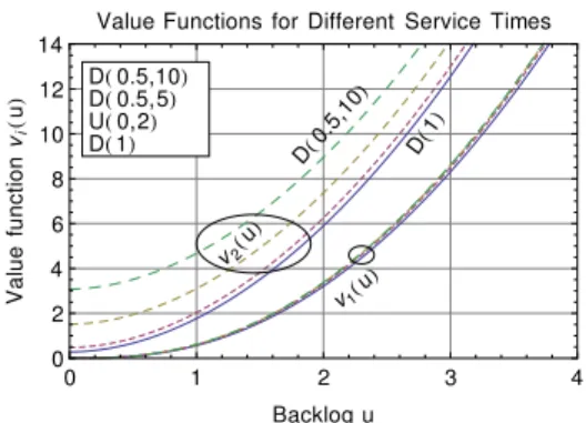
v2Hu L v1Hu L DH0.5,10L DH0.5,5L UH0,2L DH1L DH0. 5,10 L DH1 L 0 1 2 3 4 0 2 4 6 8 10 12 14 Backlog u V a lu e fu n c ti o n vi H u L
Value Functions for Different Service Times
Figure 5: Value function vi(u) for m=2 phases
(i=1,2) when service times obey D(0.5,10), D(0.5,5), U(0,2) and D(1) with unit mean and
λ=1.6. For both v1(u) and v2(u), service time
dis-tribution D(0.5,10)corresponds to the highest curve and D(1) to the lowest (in the order of variability).
sume that x1 < 1 < x2 so that with a suitable choice
of point probabilities the mean is equal to one. Similarly, D(x) denotes the deterministic distribution with one out-comex andU(x1, x2) the uniform distribution on interval
(x1, x2). Fig. 5 illustrates the resulting value functions with
D(0.5,10), D(0.5,5), U(0,2) andD(1). In each case, the mean service time is 1 and arrival rate λ = 1.6. We can observe that the higher the variance in the service times is, the higher the initial differencev2(0)−v1(0) is. The v1(u)
behave rather similarly (note the initial choicev1(0) = 0).
Consequently, we have the following result:
Corollary 6. The value function for an Erl(m, λ )/G/1-FCFS queue w.r.t. waiting time (or delay) is not insensitive to the job size distribution (form >1).
Proof. See Fig. 5.
We note that this is in contrast to the M/G/1-FCFS queue, which value function is insensitive to the job size distribution [21]. This implies that the value function of the correspond-ing Round-Robin system, due to the decomposition, is also sensitive to the job size distribution, which again is not the case if the routing is by any state-independent (static) policy such as the random Bernoulli-split.
3.
TASK ASSIGNMENT PROBLEM
In this section, we consider the system ofmparallel servers with job- and server-specific service fees and holding costs. As reference routing policies, we consider the following:
RR: Round-Robin assigns the jobs using a predefined se-quences1, s2, . . . , sm, s1, s2, . . .wheresi6=sjfori6=j. RND: Bernoulli-split assigns jobs randomly and
indepen-dently using probabilitiesp1, . . . , pm.
JSQ: Join-the-shortest-queue assigns a new job to queue with the least number of jobs.
LWL: Least-work-left assigns a new job to the queue with the shortest backlog.
Myopic chooses the queue that minimizes the costs assum-ing no other jobs arrive in future.
Ties are broken in favor of the queue with a smaller index.
3.1
Policy Iteration
The policy iteration is a standard technique of the MDP framework to improve a given policy based on a value func-tion [4, 19, 28]. In layman’s terms, at every state, it chooses the actionafor which the sum of the immediate cost and the change in the future cumulative costs is the smallest. In our case, the immediate cost of Jobj is the sum of the service feesaj and the waiting timewaj times the holding costhaj,
saj+w a j·h
a j,
where we have made it explicit that also the service fee and holding cost may depend on the chosen queue, not just on the job. Note also that with FCFS, the waiting timewjagets
fixed at the task assignment by actiona (the later arriving jobs do not affect the sojourn time of the present jobs). If the basic policy is RR, then an action may define two things:
1. The queue for the new job.
2. The future RR sequence (the phases for queues).
Similarly, utilizing (19), the expected increase in the holding costs incurred in the future is
˜
v(z⊕a)−˜v(z) =λ(v(z⊕a)−v(z)) E[H], where zis the current state of the system,z⊕a the state after actiona, andv(z) is the value function with respect to the virtual waiting time. The improved policyα0is then
α0(j,z) = argmin a∈A saj+w a jh a j+ (˜v(z⊕a)−v˜(z)) , (20)
whereAdenotes the set of possible actions (themservers). We will utilize (20) in the next section.
3.2
Numerical Examples
Let us considerm= 2 equally fast servers. First we as-sume a constant service time and then we experiment with some other elementary service time distributions.
3.2.1
Two Policy Iteration Steps
As RR/LWL is optimal with respect to the mean delay for M/D/m, let us consider a system with arbitrary job-specific holding cost rates. Let h denote the holding cost rate of the new job. If h > E[H], the intuition suggests that the new job should be assigned to the shorter queue according to RR/LWL. However, ifh <E[H], it may be beneficial to assign the new job to the longer queue, thus keeping the other queue shorter for later arriving, possibly more impor-tant, jobs. The potential pitfall is that no such “important” job arrives and one of the servers is unnecessarily idle (which never happens with RR/LWL). For the policy improvement, it is more convenient to consider the waiting time based cost structure and (20).
Let us start with the state-independentBernoulli-split pol-icy. With two identical servers, this policy assigns the new job to Server 1 with probability of 0.5, and otherwise to Server 2. The value function of the whole system is [21]
˜ vRND(u1, u2) = λ0E[H] 2(1−ρ0)(u 2 1+u 2 2),
whereλ0 is the queue-specific arrival rate,λ0=λ/2, andρ0 the queue-specific load,ρ0 =λ/2·∆. The mean difference
Figure 6: States in the diagonal where SPI suggests assigning the new Job j with holding cost hj to the
longer queue (assuming RR afterwards).
in the expected costs between assigning the new job with holding costhto Server 1 and Server 2 is
∆c=h(u1−u2) + ˜vRND(u1+∆, u2)−˜vRND(u1, u2+∆) = h+λ∆ E[H] 2−λ∆ ·(u1−u2),
i.e., ∆c is negative when u1 < u2, and vice versa. This
means that thefirst policy iteration(FPI) step (20), choos-ing the action with the lowest expected overall cost if the consecutive decisions are according the basic policy (Bernoulli-split), yields LWL. Moreover, we recall that LWL was equiv-alent to RR with a constant service time ∆.
As the first policy iteration step yielded RR (that was equivalent to LWL in this case), the value function of which we can now compute, we can proceed further and carry out thesecond policy iteration step (SPI),
RND =P I⇒ LWL =P I⇒ SPI.
Fig. 6 illustrates the regions in the state space where SPI chooses the alternative action, i.e., assigns the new job to the longer queue. The arrival rateλwas chosen to be 0.5. We note that SPI changes the FPI policy (RR) only near the diagonal where both queues have roughly equal amount of unfinished work. Higher the holding costhof the new job is, higher the backlogs must be before the change, on average, pays off. Jobs withh≥E[H] are categorically assigned to the shorter queue.
3.2.2
Two Servers with Varying Service Fees
Let us next consider a server system with primary and secondary server with fixed size jobs illustrated in Fig. 7. The servers are equally fast, i.e., the service time of a job is the same in both queues. The cost structure is
H= 1, and S1= 1, S2= 4,
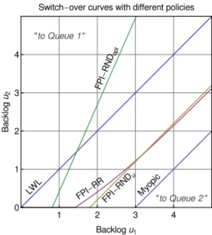
i.e., the secondary server has a four times higher service fee. Alternatively, the secondary server costs, say 3 dollars per job, the primary server is free, and the jobs incur costs at the rate of 1 dollar per unit time during their sojourn time. Note that without service fees, LWL/RR are optimal minimizing the mean waiting and sojourn times.
With two servers, both LWL and Myopic are clearly the so-called switch-over policies that can be defined by a curve
FCFS FCFS κ = 1 κ = 4 Secondary Primary λ Routing
Figure 7: Primary and secondary server with unit holding cost H=1 and service fees S1=1 and
S2=4 processing jobs with constant service time.
" to Queue 1" " to Queue 2 " LW L FP I -RN Dop t FP I-RND u FPI -RR Myo pic 1 2 3 4 0 1 2 3 4 Backlogu1 B a c k lo g u2
Switch-over curves with different policies
Figure 8: Dynamic switch-over policies illustrated for a system with a constant service time, and two equally fast servers with service fees S1=1 and
S2=4. Each policy assigns a new job to Queue 1
when the current state is above the corresponding curve, and otherwise to Queue 2.
f(u1) such that a new job is routed to Queue 2 ifu2< f(u1),
and otherwise to Queue 1. It turns out that also the FPI policies based on RND and RR yield a switch-over policy. Fig. 8 illustrates the switch-over curves forλ= 0.8. RNDopt
uses the optimal splitting probabilities, and RNDusplits the
jobs equally, p1 =p2 = 0.5. We note that the curves with
FPI-RND policies are straight lines, while with FPI-RR the switch-over curve is a slowly turning curve. Simulating the system gives the mean costs per job:
LWL: 2.20 FPI-RNDopt: 1.92
Myopic: 2.12 FPI-RNDu: 1.91
FPI-RR: 1.88
We observe that FPI-RR achieves the lowest mean cost rate, closely followed by the other two FPI policies. Numerically experimenting one can see that when λ approaches 2 (the stability bound for this system), all FPI policies converge to LWL. Similarly, whenλ→0, Myopic is optimal and all three FPI policies reduce to it.
3.2.3
Varying Holding Cost and Service Times
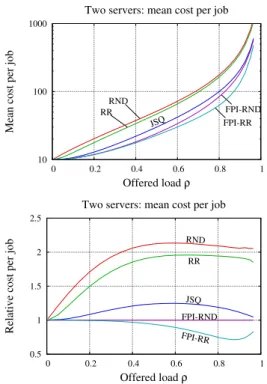
Let us consider an elementary system comprising two iden-tical servers. Jobs arrive according to the Poisson process with rate λ. Job sizes and holding costs are i.i.d. random variables. The job size is 1 with probability of 0.9, and oth-erwise 91, so that E[X] = 10 and the variance much higher.4
4
We experimented also with uniform distribution, but the results were boring as the differences between RR, LWL, and FPI-RR were small. In this respect, uniform
10 100 1000
0 0.2 0.4 0.6 0.8 1
Mean cost per job
Offered load ρ
Two servers: mean cost per job
RND RR JSQ FPI-RND FPI-RR 0.5 1 1.5 2 2.5 0 0.2 0.4 0.6 0.8 1
Relative cost per job
Offered load ρ Two servers: mean cost per job
RND RR
JSQ FPI-RND FPI-RR
Figure 9: Mean holding costs in the elementary ex-ample setting with two identical servers. FPI-RR achieves clearly the lowest cost rate.
The holding costs are assumed to obey exponential distri-bution with unit mean,H∼Exp(1).
Simulation results are depicted in Fig. 9 for Bernoulli-split (RND), JSQ, RR, FPI-RND (i.e., LWL) and FPI-RR. The offered loadρis on thex-axis, and they-axis corresponds to the mean costs incurred per job. The first figure shows the absolute performance in logarithmic scale, and the second the performance relative to LWL. Note that LWL minimizes the holding cost of the current job, i.e., it makes the same greedy decision as selfish users do.
Whenρ ≈0, LWL and JSQ both, obviously, work well. The task there is merely to avoid situations when two or more jobs are in one server while the other server is idle. As ρincreases beyond about 0.1, the performance of JSQ starts to degrade. At ρ≈0.4 or higher, also the performance of LWL, due to its greedy behavior degrades. Aroundρ= 0.9, FPI-RR is about 25% better than LWL. As ρ → 1, JSQ, LWL and FPI-RR appear to converge to the same point. Indeed, at that limit the mean queue lengths explode and it is sufficient to (dynamically) balance the load.
4.
MORE ADVANCED APPLICATIONS
The ability to determine a value function for Erl/G/1 queues enables the analysis of far more complex server sys-tems than the plain Round-Robin system. One example is illustrated in Fig. 10(a), where a multi-layer RR is con-structed: Queue 1 behaves according to Erl(2, λ)/G/1 and Queues 2 and 3 according to Erl(4, λ)/G/1. This type of arrangements can be advantageous when the service rates tion is sufficiently close to a constant value. The chosen job size distribution has sufficiently high variance so that it is important to take into account jobs arriving in the future.
Round Robin Round Robin FCFS FCFS FCFS λ (a) Round Robin small variance FCFS FCFS FCFS λ SITA short long (b)
Figure 10: (a) Multi-layer round-robin system feeds tasks to each queue with Erlang-distributed inter-arrival times. (b) In the hybrid system, Queue 1 behaves according to M/G/1 and Queues 2 and 3 according to Erl(2,λ0)/G/1 with reduced variance in the service times.
and/or operating costs are asymmetric.
The main strength in RR comes from the fact that it reduces the variability in the inter-arrival times (see Sec-tion 2.4.5). On the other hand, a high variability in the job sizes can be equally harmful (due to the second moment in the Pollazcek-Khinchine formula for the mean waiting time). The so-called Size-Interval-Task-Assignment (SITA) policy [7, 16, 10, 17] seeks to reduces the variability in the job sizes by assigning jobs with a similar size to the same queue. To this end, the support of the job sizes is divided intom non-overlapping intervals [ξi, ξi+1),i= 1, . . . , m, and a job with
sizexis assigned to Serveriiffx∈[ξi, ξi+1).
Fig. 10(b) illustrates a server system which combines the worthwhile features of SITA (variance reduction in service times) and RR (which was the optimal policy w.r.t. delay for tasks with a constant service time). The arrival pro-cess to Queue 1 is a Poisson propro-cess as SITA is a state-independent policy. Queues 2 and 3 behave according to Erl(2, λ0)/G/1, where the service time of tasks can have a significantly smaller variance thanks to SITA. Moreover, dedicated jobs arriving according to some other Poisson pro-cess can be directed to any point already receiving a Poisson process, such as the Queue 1 and the second level RR dis-patcher in Fig. 10(b). Thus, the analysis of systems that hierarchically combine dispatchers remains tractable, their value function can be determined, and the policy improve-ment step can be carried out.
5.
CONCLUSIONS
We have analyzed the Round-Robin (RR) routing to a system of parallel queues. RR is a commonly used robust technique to balance the load by assigning tasks to different servers sequentially. It decreases the burstiness in the arrival process to each queue, which is important especially when the queues process the jobs in FCFS order.
The availability of the value function for RR-systems, via the corresponding value function of Erl/G/1 queues, pro-vides new insight to this mechanism itself (and to G/G/1
queues). The value functions that we considered character-ize the system state with respect to the service fees and vir-tual waiting time, and also enable the policy iteration step with respect to a very versatile cost structure defined by job-and server-specific service fees job-and holding costs, yielding ro-bust cost- and state-aware routing policies. Moreover, as an useful side-product, we obtain the mean waiting time in the Round-Robin system, which itself is a non-trivial result even for an M/D/m-RR queue.
Acknowledgments
This work was supported by the Academy of Finland in the Top-Energy project (grant no. 268992) and the PDP project (grant no. 260014).
6.
REFERENCES
[1] O. Akgun, R. Righter, and R. Wolff. Multiple server system with flexible arrivals.Advances in Applied Probability, 43:985–1004, 2011.
[2] P. S. Ansell, K. D. Glazebrook, and C. Kirkbride. Generalised ’join the shortest queue’ policies for the dynamic routing of jobs to multi-class queues.The J. of the Oper. Res. Society, 54(4):379–389, Apr. 2003. [3] Y. Arian and Y. Levy. Algorithms for generalized
round robin routing.Oper. Res. Lett., 12(5):313–319, 1992.
[4] R. Bellman.Dynamic programming. Princeton University Press, 1957.
[5] S. Bhulai. On the value function of the M/Cox(r)/1 queue.Journal of Applied Probability, 43(2):363–376, June 2006.
[6] C. D. Crommelin. Delay probability formulas when the holding times are constant.Post Office Electrical Engineers Journal, 25:41–50, 1932.
[7] M. E. Crovella, M. Harchol-Balter, and C. D. Murta. Task assignment in a distributed system: Improving performance by unbalancing load. InProceedings of SIGMETRICS ’98, pages 268–269, Madison, Wisconsin, USA, June 1998.
[8] D. Down and R. Wu. Multi-layered round robin routing for parallel servers.Queueing Systems, 53(4):177–188, 2006.
[9] A. Ephremides, P. Varaiya, and J. Walrand. A simple dynamic routing problem.IEEE Transactions on Automatic Control, 25(4):690–693, Aug. 1980. [10] H. Feng, V. Misra, and D. Rubenstein. Optimal
state-free, size-aware dispatching for heterogeneous M/G/-type systems.Performance Evaluation, 62(1-4):475–492, 2005.
[11] G. J. Franx. A simple solution for the M/D/c waiting time distribution.Oper. Res. Lett., 29(5):221–229, Dec. 2001.
[12] G. J. Franx. The transient M/D/c queueing system, 2002.
[13] B. Hajek. The proof of a folk theorem on queuing delay with applications to routing in networks.J. ACM, 30(4):834–851, Oct. 1983.
[14] B. Hajek. Extremal splittings of point processes.
Mathematics of Oper. Res., 10(4):543–556, Nov. 1985. [15] M. Harchol-Balter.Performance Modeling and Design
of Computer Systems: Queueing Theory in Action.
Cambridge University Press, 2013.
[16] M. Harchol-Balter, M. E. Crovella, and C. D. Murta. On choosing a task assignment policy for a distributed server system.Journal of Parallel and Distributed Computing, 59:204–228, 1999.
[17] M. Harchol-Balter, A. Scheller-Wolf, and A. R. Young. Surprising results on task assignment in server farms with high-variability workloads.ACM SIGMETRICS Performance Evaluation Review, 37:287–298, 2009. [18] A. Hordijk and G. Koole. On the optimality of the
generalised shortest queue policy.Prob. Eng. Inf. Sci., 4:477–487, 1990.
[19] R. A. Howard.Dynamic Probabilistic Systems, Volume II: Semi-Markov and Decision Processes. Wiley, 1971. [20] E. Hyyti¨a, S. Aalto, and A. Penttinen. Minimizing
slowdown in heterogeneous size-aware dispatching systems.ACM SIGMETRICS Performance Evaluation Review, 40:29–40, June 2012.
[21] E. Hyyti¨a, A. Penttinen, and S. Aalto. Size- and state-aware dispatching problem with queue-specific job sizes.European J. of Oper. Res., 217(2), 2012. [22] E. Hyyti¨a, S. Aalto, A. Penttinen and J. Virtamo. On
the value function of the M/G/1 FCFS and LCFS queues.J. of Applied Probability, 49(4), 2012. [23] A. J. E. M. Janssen and J. S. H. Van Leeuwaarden.
Back to the roots of the M/D/s queue and the works of Erlang, Crommelin and Pollaczek.Statistica Neerlandica, 62(3):299–313, 2008.
[24] G. Koole, P. D. Sparaggis, and D. Towsley. Minimizing response times and queue lengths in systems of parallel queues.Journal of Applied Probability, 36(4):1185–1193, Dec. 1999. [25] K. R. Krishnan. Joining the right queue: a
state-dependent decision rule.IEEE Transactions on Automatic Control, 35(1):104–108, Jan. 1990. [26] Z. Liu and R. Righter. Optimal load balancing on
distributed homogeneous unreliable processors.
Operations Research, 46(4):563–573, 1998.
[27] Z. Liu and D. Towsley. Optimality of the round-robin routing policy.Journal of Applied Probability, 31(2):466–475, June 1994.
[28] M. L. Puterman.Markov Decision Processes: Discrete Stochastic Dynamic Programming. Wiley, 2005. [29] P. D. Sparaggis and D. Towsley. Optimal routing and
scheduling of customers with deadlines.Prob. Eng. Inf. Sci., 8(1):33–49, 1994.
[30] H. Tijms. New and old results for the M/D/c queue.
AE ¨U - International Journal of Electronics and Communications, 60(2):125–130, 2006.
[31] D. Towsley, P. Sparaggis, and C. Cassandras. Stochastic ordering properties and optimal routing control for a class of finite capacity queueing systems. InProc. of the 29th IEEE Conference on Decision and Control, pages 658–663, Dec. 1990.
[32] R. R. Weber. On the optimal assignment of customers to parallel servers.Journal of Applied Probability, 15(2):406–413, June 1978.
[33] W. Winston. Optimality of the shortest line discipline.