Faisal M. Zahid & Gerhard Tutz
Multinomial Logit Models with Implicit Variable
Selection
Technical Report Number 089, 2010
Department of Statistics
University of Munich
Multinomial Logit Models with Implicit Variable Selection
Faisal Maqbool Zahida,∗, Gerhard Tutzb
aLudwig-Maximilians-University Munich, Ludwigstrasse 33, D-80539 Munich, Germany bLudwig-Maximilians-University Munich, Akademiestraße 1, D-80799 Munich, Germany
Abstract
Multinomial logit models which are most commonly used for the modeling of unordered multi-category responses are typically restricted to the use of few predictors. In the high-dimensional case maximum likelihood estimates
frequently do not exist. In this paper we are developing a boosting technique calledmultinomBoostthat performs
variable selection and fits the multinomial logit model also when predictors are high-dimensional. Since in
multi-category models the effect of one predictor variable is represented by several parameters one has to distinguish between
variable selection and parameter selection. A special feature of the approach is that, in contrast to existing approaches, it selects variables not parameters. The method can distinguish between mandatory predictors and optional predictors. Moreover, it adapts to metric, binary, nominal and ordinal predictors. Regularization within the algorithm allows to include nominal and ordinal variables which have many categories. In the case of ordinal predictors the order information is used. The performance of boosting technique with respect to mean squared error, prediction error and the identification of relevant variables is investigated in a simulation study. For two real life data sets the results are also compared with the Lasso approach which selects parameters.
Key words: Logistic regression, Multinomial logit, Variable selection, Side constraints, Likelihood-based boosting,
Penalization, Hit rate, False alarm rate.
1. Introduction
The multinomial logit model is the most frequently used model in regression analysis with categorical response. Typically, the maximum likelihood method is used for estimating the parameters. However, the use of maximum likelihood estimation severely limits the number of predictors in the multinomial logit models. As the number of covariates increases relative to the sample size, problems with the convergence of parameter estimates arise and the
usual ML estimates will not exist for p > n.To overcome the problem, one alternative is to rely on penalization
∗Corresponding author. Tel.:++49 89 2180 6408; fax.:++49 89 2180 5040.
Email addresses:[email protected](Faisal Maqbool Zahid),[email protected](Gerhard Tutz)
techniques. One of the oldest penalization techniques is ridge regression which was extended to generalized linear models (GLM) by Nyquist (1991), Segerstedt (1992). In contrast to ridge regression which shrinks the parameter estimates towards zero but does not enforce subset selection, Lasso (Tibshirani (1996)) does not only shrink the parameter estimates but also enforces subset selection by setting some of the parameter estimates exactly equal to zero. An extension to GLMs was proposed by Park and Hastie (2007). However, for multicategory responses, not much literature is available. Multinomial logistic regression with Lasso type estimates was considered by Krishnapuram et al. (2005). Friedman et al. (2010) considered L1 (Lasso), L2 (ridge) penalties and the elastic net (mixture of the L1 and L2 penalty). Zahid and Tutz (2009) used ridge regression with symmetric side constraints, which makes the ridge estimates invariant to the choice of a reference category. A general alternative to maximum likelihood estimation is likelihood-based boosting. Boosting was originally developed in the machine learning community to improve classification (e.g., Schapire (1990) and Freund and Schapire (1996)). Friedman et al. (2000) showed that boosting can also be viewed as an approximation to additive modeling using the appropriate likelihood function. B¨uhlmann
and Yu (2003) used theL2loss function instead of the LogitBoost cost function within the context of linear models.
B¨uhlmann (2006) showed the relation to Lasso which also does variable selection and shrinkage without making any assumptions about the correlation structure of the predictors. For an overview on boosting see B¨uhlmann and Hothorn (2007). Likelihood-based boosting based on one step of Fisher scoring for variable selection in generalized additive models (GAM) was proposed by Tutz and Binder (2006).
In this article we are using the likelihood based boosting technique with one step of Fisher scoring for variable selection in multinomial logit models. For the weak learners we are using the ridge penalty. When seeking for a parsimonious model, one frequently considers some of the covariates as an essential part of the model. For example,
in a treatment study one is interested in particular in the treatment effect, which is considered a mandatory covariate.
The other covariates which might be of relevance are considered as optional. Similar to Tutz and Binder (2007) our method distinguishes between mandatory and optional predictors.
When working with categorical covariates it is essential that selection does not refer to parameters but to covariates (comprising the group of parameters associated with the categorical covariate). Consequently, our approach performs
variable selection in terms of covariates rather than parameters. For this purpose our approach differentiates among the
categorical predictors that contain a group of parameters (for each logit) in the parameter space and those predictors having only one parameter for each logit of the multinomial logit model e.g., binary or metric predictors. Moreover, in
the case of ordinal covariate(s), rather than penalizing the parameters, our approach penalizes the differences between
the paramters of the adjacent categories.
In Section 2 the side constraints for the multinomial logit model and the regularization for different types of covariates
are discussed . Boosting is discussed in Section 3, Section 4 gives empirical results of a simulation study. The algorithm is applied to real life data set and the results are compared with those obtained from the Lasso approach in Section 5.
2. Predictor Space, Side Constraints and Regularization
In this section we describe the different types of candidate predictors (candidates to become part of a parsimonious
logit model) which will be used in Section 3, and how they are incorporated into the boosting algorithm for subset
selection. For simplicity, we assume in this section that the multinomial logit model has only one predictor withK
parameters to be estimated for each of thekcategories of the response variable. If the predictor is metric or binary
thenK=1, andK>1 if the predictor is a multicategory variable with theK+1 categories labeled as 1, . . . ,K,K+1.
Although the intercept is part of the model, for simplicity in the following the intercept is omitted.
2.1. Side Constraints for the Multinomial Logit Model
Let the response variableY ∈ {1, . . . ,k}havekpossible categories. The generic form of the multinomial logit model
is P(Y =r|x)= exp(x Tβββ r) Pk s=1exp(xTβββs) = Pkexp(ηr) s=1exp(ηs) , (1)
whereβββTr =(βr1, . . . , βrK).Since parametersβββT1, . . . , βββTk are not identifiable, for the identifiability of parameters one
has to specify additional constraints. One most commonly used side constraint is to choose one of the response
categories as reference category. If categorykis chosen as reference, then one sets
βββTk =(0, . . . ,0) yielding ηk=0.
Of course, any category can be chosen as a reference category. With categorykas the reference category, the model is
P(Y =r|x)= exp(x
Tβββ r)
1+Pqs=1exp(xTβββs) for r
=1, . . . ,q. (2)
withq=k−1.Alternatively one can work with the symmetric side constraint. Withβββ∗sdenoting the parameter vector
for categorys,it is given by
k X
s=1
βββ∗s=0. (3)
Then the multinomial logit model has the form
P(Y=r|x)= exp(x Tβββ∗ r) Pk s=1exp(xTβββ∗s) = exp(η ∗ r) Pk s=1exp(η∗s) for r=1, . . . ,q (4)
With symmetric side constraint, the median response defined by the geometric mean can be viewed as the
refer-ence category. The parametersβββ∗ have a different interpretation than βββ obtained with a reference category
con-straint. Hereβββ∗rreflects the effects ofxon the logits whenP(Y =r|x) is compared to the median responseGM(x)=
k
qQk
s=1P(Y =s|x).
In the following, letβββT =(βββT1, . . . , βββTq,0) andβββ∗T =(βββ∗1T, . . . , βββ∗kT) represent the parameter vectors for the multinomial
logit model under the reference category side constraint (βββk=0) and symmetric side constraint (Pks=1βββ∗s =0),
is by consideringβββT.j=(β1j, . . . , βk−1,j), and βββ.∗Tj =(β∗1j, . . . , β∗k−1,j), j=1, . . . ,K, which denote parameter vectors
for a particular variable with reference categorykor symmetric side constraints respectively, then
βββ∗.j=Tβββ.j for j=1, . . . ,K, (5)
whereTis aq×qmatrix (q=k-1) with diagonal elements qk and off-diagonal elements as−1k.The matrixT−1,then,
has the diagonal enteries as 2 and all off-diagonal elements are 1.For likelihood (or penalized likelihood) estimation,
the complete design matrixXof orderq(n×K) is given byXT =X1 X2 . . . X
n. The matrixXiis aq×Kdesign
matrix composed ofxiand is given by
Xi= xT i xT i . .. xT i .
Since the parametersβββ∗is a reparameterization of the parametersβββ,the computation of maximum likelihood estimates
ofβββ∗needs a transformation of the design matrixXasX∗=XT∗,for aq(K×K) matrixT∗given byT∗=T−1
q×q⊗IK×K,
where⊗is the Kronecker matrix product. If not mentioned otherwise we will use the symmetric side constraint.
2.2. Regularization and Type of Predictors
In the version of componentwise boosting used in Section 3, the effect of one predictor variable, that is all the
pa-rameters linked to that variable, will be updated within one step of the algorithm. Updating of the predictor will be performed by regularized estimates with the regularization depending on the type of predictor.
Nominal Predictors
Let the predictorXtake values 1, . . . ,K,K+1 andXbe the only variable in the predictor. The parameter values for
response categoryrhave lengthKand are given byβββ∗rT =(β∗r1, . . . , β∗rK).Regularization will be based on ridge type
estimates. For the multinomial logit model it is advisable to use the symmetric side constraint, otherwise shrinkage is determined by the choice of the reference category (see Zahid and Tutz (2009)). The corresponding ridge estimators can be motivated by maximization of the penalized log-likelihood
lp(βββ)= n X i=1 li(βββ)−λ 2 k X r=1 K X j=1 β∗r j2,
whereli(βββ) is the log-likelihood contribution of theith observation,λis a tuning parameter andPkr=1β∗r j =0. The
underlying penalty can also be given by
J(βββ∗)= k X r=1 K X j=1 β∗r j2= K X j=1 βββ∗.jTT−1βββ∗.j, (6) 4
with shortened vectorβββ∗.jT =(β∗1j, . . . , β∗q j).It should be noted that the use of matrixT−1in place of an identity matrix
I,implicitly penalizes the size of parameters for allkresponse categories while working with theq = k−1 logits.
In matrix notation, one obtains the ridge penalty with symmetric side constraint, for a complete design matrix for the multinomial logit model in the form
J(βββ∗)=βββ∗TT∗βββ∗,
whereβββ∗is aqK×1 vector given byβββ∗T =(βββ∗1T, . . . , βββq∗T) and the matrixT∗ =Tq−×1q⊗IK×K,is same as discussed in
Section 2.1.
Ordinal Predictors
In regression analysis, ordinal predictors are often part of the predictor space but proper treatment is found rarely. If the multinomial logit model has some ordinal predictors, penalization should account for the order of the categories.
With ordinal predictors, it is advantageous to penalize the differences between the coefficients of adjacent categories
rather than penalizing the size of the parameters themselves. By penalizing such differences, one gets a smoother
coefficient vector and avoid the high jumps among the parameter estimates corresponding to the ordinal covariate
(see Gertheiss and Tutz (2009)). Let again the ordinal predictor takeK+1 categories 1, . . . ,K,K+1 and let the first
category serve as reference category such thatβ.1=0.Then for ordinal predictor withK+1 categories an appropriate
penalty with symmetric side constraint is
J(βββ∗)= k X r=1 K+1 X j=2 (β∗ r j−β∗r,j−1)2. (7)
If one works with a reference category constraint then the penalty is simply given asJ(βββ)=Pkr=1PKj=+21(βr j−βr,j−1)2,
or in matrix notationJ(βββ)=PKj=+21βββT.jΩΩΩβββ.j,where ΩΩΩ =UTUwithU,aK×Kmatrix, given by
U= 1 0 · · · 0 −1 1 . .. ... 0 −1 1 . .. ... .. . . .. ... ... 0 0 · · · 0 −1 1
But we are proceeding with symmetric side constraint where we have to penalize the differences between the
param-eters of adjacent categories for allkcategories of the response variable, while working withqlogits. In such case the
penalty term for the complete design matrix is given as
whereβββ∗is aqK×1 vector given byβββ∗T = (βββ∗1T, . . . , βββ∗qT) and the matrixΩΩΩ∗ = T−q×1q⊗ΩΩΩK×K.The matrixΩΩΩ∗ will
handle implicitly the penalization of differences between the adjacent categories forkcategories while working with
theqlogits.
In the next section where we are using the ridge type penalties to obtain weak learners in the boosting algorithm. Two
types of penalty matrices are used for the expressionJ(βββ∗).If the candidate predictor is ordinal, the penalty matrixΩΩΩ∗
is used to penalize the differences among the coefficients of adjacent predictor categories forkresponse categories and
if the candidate predictor is nominal, the penalty matrixT∗is used to penalize the size of the parameters. Although
we are working withqlogits both penalty matrices implicity perform the penalization for theklogits under symmetric
side constraint.
3. Boosting
The method proposed in this section is based on likelihood-based boosting with quadratic penalties for regularization to obtain weak learners. Let us consider the multinomial logit model with side constraint given by (3) and the penalty term given by (6) or (8) according to the nature of predictors. Then the penalized log-likelihood is
lp(βββ∗)= n X i=1 li(βββ∗)−λ 2J(βββ∗)= n X i=1 li(βββ∗)−λ 2βββ∗TP∗βββ∗
with penalty matrixP∗which will be replaced byT∗orΩ∗depending on the nature of the predictors. The
correspond-ing penalized score functionsp(βββ∗) is given by
sp(βββ∗) = n X i=1 X∗T i Di(βββ∗)ΣΣΣ−i1(βββ∗)[yi−h(ηηη∗i)]−λP∗βββ∗ = X∗TD(βββ∗)ΣΣΣ−1(βββ∗)[y−h(ηηη∗)]−λP∗βββ∗,
whereβββ∗is a vector of parameters of lengthq×(p+1) andX∗is the transformation of the actual design matrix as
discussed in Section 2.2. The matrixDi(βββ∗) = ∂h(ηηη
∗
i)
∂ηηη∗ is the derivative ofh(ηηη∗) evaluated atηηη∗i = X∗iβββ∗andΣΣΣ(βββ∗) =
cov(yi) is the covariance matrix ofith observation ofygiven parameter vectorβββ∗. For the full design matrix, in matrix
notationyandh(ηηη∗) are given byyT =(yT
1, . . . ,yTn) andh(ηηη∗)T =(h(ηηη∗1)T, . . . ,h(ηηη∗n)T) respectively. The matrices have
block diagonal formΣΣΣ(βββ∗)=diag(ΣΣΣ−i1(βββ∗)), W(βββ∗)=diag(Σ−i1(βββ∗)), andD(βββ∗)=diag(Di(βββ∗)).
For the boosting algorithm, let the the whole predictor space be dichotomized into two non-overlapping groups.
One group contains the mandatory/obligatory covariates (including the intercept) which are the essential part of the
model and are necessarily re-estimated in each ofmboosting iterations. The second group consists of the candidate
predictors each of which is a candidate to become a part of the final parsimonious model decided aftermboosting
iterations. Let the predictor variable indicesV ={1, . . . ,p}be partitioned into disjoint sets asV =Vo∪V1∪. . .∪Vg,
whereVo represents the obligatory predictors (each predictor may have one or more parameters associated with it)
andV1, . . . ,Vg are g predictors, among which we want to make a subset selection. Let Kj denote the number of
parameters/dummies for one logit associated with the predictor Vj, (j = 1, . . . ,g).So the total predictor space is
partitioned into two disjoint sets of obligatory and candidate predictors i.e.,V =Vo∪Vc,whereVc=V1∪. . .∪Vg,
and the split of complete parameter vector is then given asβββ∗T =(βββ∗oT βββ∗cT).For the re-fitting process a combination
of mandatory and some candidate predictor is considered i.e.,Vo ∪Vj, j ∈ {1, . . . ,g},will be considered in a
re-fitting process in a particular boosting iteration. If among the candidate predictors,Vjis considered for re-fitting in a
boosting iteration then for likelihood/penalized-likelihood estimation we use theq(n×Kj) design matrixXjfrom the
full design matrix of orderq(n×(Ppj=1Kj+1)).The design matrixXjis based on the parameters/columns associated
withVjand is given as
XT j =X1(j) X2(j) . . . Xn(j) with Xi(j)= xT i(j) xT i(j) . .. xT i(j) (9)
ThemultinomBoostalgorithm can be described as follows:
Algorithm:mulinomBoost
Step 1: (Initialization)
Fit the intercept modelµµµ∗0=h(ηηη∗0) by maximizing the likelihood fucnction to obtain ˆηηηˆˆ∗0andh(ˆηηηˆˆ∗0).
Step 2: Boosting iterations
Form=1,2, . . .
Step 2A: For obligatory/mandatory predictors
(i) Fit the modelµµµ=h(ˆηηηˆˆm∗−1+X∗oβββo∗F1),where ˆηηηˆˆm∗−1is treated as an offset andX∗ois the design matrix based on the
parameters/columns corresponding toVo. βββ∗oF1is computed with one-step Fisher scoring as
βββo∗F1 = (X∗oTW(ˆηηηˆˆ∗m−1)X∗o)−1Xo∗TW(ˆηηηˆˆ∗m−1)D−1(y−µµµˆˆˆ∗m−1).
(ii) set ˆηηηˆˆ∗m=ηηηˆˆˆ∗m−1+X∗oβββ∗oF1.
(iii) setβββ∗o(m) =βββo∗(m−1)+βββ∗oF1 Step 2B: For candidate predictors
(i) For j=1, . . . ,g,fit the modelµµµ=h(ˆηηηˆˆ∗m+X∗jβββ∗jF1),with offset ˆηηηˆˆ∗mandX∗
jis the design matrix corresponding to
Vj.With one-step Fisher scoring by maximizing penalized log-likelihood,βββ∗jF1is computed as
βββ∗jF1= (X∗jTW(ˆηηηˆˆ∗m)X∗j+νΛΛΛ)−1X∗jT W(ˆηηηˆˆ∗m)D−1(y−µµµˆˆˆ∗m).
whereν= pd fjλwith ridge penaltyλ.The penalty matrixΛΛΛis given as:
Λ Λ Λ = ΩΩΩ ∗ if Vjis ordinal T∗ otherwise.
(ii) From the candidate predictorsV1, . . . ,Vg,select the predictor sayVbest,which improves the fit maximally and set βββ∗cF1= βββ ∗F1 j if j∈Vbest 0 if j<Vbest. (iii) set ˆηηηˆˆ∗m←ηηηˆˆˆ∗m+X∗cβββ∗cF1. (iv) setβββ∗c(m)=βββc∗(m−1)+βββ∗cF1
In the above algorithm, for regularization, multiplying the ridge penaltyλwith pd fj accounts for the number of
parameters,d fj,involved in the candidate predictor. The parameterλis chosen large in order to obtain a weak learner.
If it is chosen large enough, as usually in boosting, the performance does not depend on the choice of the value ofλ,
it only influences the needed number of iterations. In step 2B of the algorithm, the deviance can be used for selecting
a candidate predictor for refit. In themth boosting iteration, that candidate predictor will be considered for the refit
which has minimum deviance i.e., Dev(ˆηηη∗m).As the candidate predictors may have a varying number of parameters, an
alternative criterion for predictor selection is Akaike’s information criterion (AIC) or Bayesian information criterion (BIC) because both of these measures also take the the number of parameters into account. The AIC criterion is given by
AIC=Dev(ˆηηη∗m)+2d fm
whereas the BIC criterion is given by
BIC=Dev(ˆηηη∗m)+log(qn)d fm
whered fmis the effective degrees of freedom given by the trace of the hat matrix. But if the deviance as a criterion for
the selection of a covariate makes the fitting procedure much faster, especially for large samples that is an advantage. The stopping criteria can be based on deviance based cross-validation, which we are using. Alternative but more time-consuming options are AIC or BIC.
One possible drawback of boosting is that the parameters corresponding to some predictors may be updated only once or twice within the boosting iterations. It is recommended to select only those variables whose estimates are not too
small compared to the other estimates. ThemultinomBoostalgorithm sets all the parameter estimates corresponding
to theith predictor equal to zero, if
1 k.Ki PKi j=1 Pk l=1|βi jl| Pp i=1 1 k.Ki PKi j=1 Pk l=1|βi jl| < 1 p, (10)
aftermboosting iterations. For boosting, by using approximate hat matrixHmat the end ofmth boosting iteration,
AIC and BIC criteria are given as AIC=Dev(ˆηηη∗m)+2 tr(Hm) and BIC=Dev(ˆηηη∗m)+log(qn) tr(Hm) respectively. The
approximate hat matrix used in themth boosting iteration is discussed in the following proposition.
Proposition:In themth boosting iteration, an approximate hat matrix for which ˆµµµ∗m≈Hmyis given by Hm= m X j=0 Mj j−1 Y i=0 (I−M0),
where for the multinomial logit models withWm=Dm(forWm=W(ˆηηη∗m) andDm=D(ˆηηη∗m)),Mm=Wm(XTmWmXm+
νΛΛΛ)−1Xm.
Proof:At the end ofmth boosting iteration, letVj =Vbestis selected. For multinomial logit models withWm=Dm,
whereWm =W(ˆηηη∗m) andDm=D(ˆηηη∗m),we have ˆηηηm−ηηηˆm−1 =(X∗jTWmX∗j+νΛΛΛ)−1X∗jT (y−µµµˆˆˆ∗m−1).By using the first
order Taylor approximation of first order i.e.,h(ˆηηη)≈h(ηηη)+(∂h(ηηη)/∂ηηηT)(ˆηηη−ηηη),we obtain ˆµµµ∗m≈µµµˆ∗m−1+Wm(ˆηηη∗m−ηηηˆ∗m−1)=
ˆ µ µµ∗m−1+WmX∗jβββˆ∗ F1 =µµµˆ∗m−1+WmX∗j(X∗jTWmX∗j+νΛΛΛ)−1X∗jT(y−µµµˆˆˆ∗m−1).So we have ˆµµµ∗m≈µµµˆm∗−1+Mm(y−µµµˆˆˆ∗m−1) with Mm=WmX∗j(X∗jTWmX∗j+νΛΛΛ)−1X∗jT.We can write ˆµµµ∗mas ˆµµµ∗m≈µµµˆ∗m−1+Mm(y−µµµˆˆˆm∗−1)=Hm−1y+Mm(I−Hm−1)y.
Expanding in the same way, for mth boosting iteration, the general form of the approximate hat matrix isHm =
Pm
j=0MjQij=−01(I−M0),with ˆµµµ∗m≈Hmyand the starting value ˆµµµ∗0=M0y.
4. Simulation Study
The performance ofmultinomBoostalgorithm is evaluated using simulated data. For a response variable with three
categories (unordered), the covariates are drawn from ap−dimensional multivariate normal distribution with mean0
and the covariance among the covariates (among the columns of covariate matrix)xjandxkisρ|j−k|.Two values ofρ,
0.3 and 0.7 are considered in the study. For each value ofρwe draw a samples of sizes 50 and 100 for a design space
of 20 covariates (16 continuous and four binary covariates). Among the 20 covariates, six covariates (five continuous and one binary covariate) are informative i.e., we have six covariates with non-zero parameters and the rest having
zero value. For the true parameter valuesβββthe totalq.Ppinfo
j=1 Kjvalues (wherepinfois the total number of informative
covariates) are obtained by the formula (−1)jexp(−2(j−1)/20) for j =1, . . . ,qPpinfo
j=1 Kj,and are randomly allotted
to the parameters corresponding to the informative covariates. The true parameter vector, then, isβββT =csnr(βββ1 βββ2),
where the constantcsnris chosen so that the signal-to-noise ratio is 3.0.The performance of themultinomBoostwith
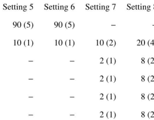
respect to the variable selection in high dimensional data sets, where the categorical covariates are also involved is also evaluated. For this purpose, we use four additional settings, for which the total number of predictors used with their type and the number of informative predictors (within the brackets) is as follows:
Type of predictor Setting 5 Setting 6 Setting 7 Setting 8
Metric (withρ=0.3 &ρ=0.7 for setting 1 & 2 respectively): 90 (5) 90 (5) − −
Binary: 10 (1) 10 (1) 10 (2) 20 (4)
Categorical (with three unordered categories): − − 2 (1) 8 (2)
Categorical (with four unordered categories): − − 2 (1) 8 (2)
Categorical (with three ordered categories): − − 2 (1) 8 (2)
Categorical (with four ordered categories): − − 2 (1) 8 (2)
For the first four settings we performedS =50 simulations per setting andS =30 simulations per setting for the last
four high dimensional settings. For the subset selection in boosting we use three criteria, deviance, AIC and BIC. For
each criterion, in each setting, a fixed value of the rigde penaltyλis used for allS simulations. We chose that value for
which the optimal number of boosting iterations was between 50 and 200.The optimal number of iterations in each
case are decided on the basis of 10−fold cross-validation. The results obtained with these three criteria are compared
to the MLE(oracle), which refers to the usual ML estimate for the model that contains the informative covariates only. Therefore MLE(oracle) has the big advantage of using the variables that carry information. In addition we consider ridge estimation (ssc-Ridge) with symmetric side constraint obtained for the model that contains all covariates. The
performance ofmultinomBoostalgorithm is evaluated in terms of mean squared error of the parameter estimates ˆβββ,
mean deviance of the fit, i.e. deviance(ˆπππ), prediction error and the identification of influential observations. The MSE
of ˆβββis computed using the estimates of allklogits as:
MSE(ˆβββ)= 1
S
X s
||βββˆs−βββ||2.
Prediction performance is evaluated by drawing a new sample (test data) of 1000 observations. In generalized linear models, the mean deviance is an appropriate measure than mean squared prediction error. For the test data set the Mean Prediction Error (MPE) based on the deviance measure is given as:
MPE= 1 S X s Ds= 1 S X s hXn i=1 k X j=1 πtesti j logπ test i j ˆ πtesti j i
The deviance for the fit is computed asPn
i=1Pkj=1yi jlog y i j ˆ πi j withyi jlog y i j ˆ πi j =0 foryi j=0.
4.1. MSE and Prediction Performance
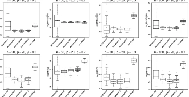
Figure 1 shows the results for the low dimensional settings in terms of MSE. Figure 2 shows the corresponding results
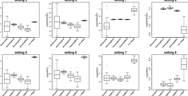
for the high-dimensional settings where the model involves categorical covariates also. For setting 8,which involves
only categorical covariates, the results of MLE(oracle) are not given because of its non-existence. The solid circles within the boxes represent the mean over observations for which the box-plots were drawn. It is seen that boosting
strongly outperforms ridge (exception setting 8 for MSE). More surprisingly mean and median values are smaller than the corresponding values of the oracle. The oracle shows much larger variation, for some data sets its performance is very bad for some rather good. But given that it uses information that is not available in practice the performance is weak.
In setting 8 which contains only categorical covariates, the results of boosting regarding MSE(ˆβββ) and the fit are
disturbed but still give better prediction performance. It should be noted that the results for boosting procedure in this case (with all covariates categorical) could be improved by using smaller value of signal-to-noise ratio. Table 1 shows
the mean of log(MSE(ˆβββ)),mean deviance of the fit i.e., deviance(ˆπ) and the mean prediction error (MPE). The values
appearing in boldface indicate the best results among all considered methods. In summary, Table 1 shows that boosting is a much better technique than its competitors not only when there is small correlation but also with high correlation
among the covariates. We are not comparing the results ofmultinomBoostwith estimates of Lasso or elastic net
such as given by Friedman et al. (2010), because our algorithm is working in a different way and performs predictor
selection (selecting a group of parameters at a time associated with a predictor) rather than parameter selection.
4.2. Identification of Informative Predictors
In addition to small prediction error (MPE) a selection procedure should yield a parsimonious model that includes all informative covariates. To identify whether the correct informative covariates are part of the final parsimonious model or not, we are using ”hit rate” and ”false alarm rate” as criteria. The hit rate is defined as the proportion of correctly identified informative predictors, given as
hit rate=
Pp
j=1I(βββtrue,j,0).I(ˆβββj,0)
Pp
j=1I(βββtrue,j,0)
.
The false alarm rate is defined as the proportion of non-informative predictors dubbed as informative, and is given as
false alarm rate=
Pp
j=1I(βββtrue,j=0).I(ˆβββj,0)
Pp
j=1I(βββtrue,j=0)
.
Hereβββtrue,j, j = 1, . . . ,p is a vector that comprises the true parameter values for thek logits associated with the
jth predictor and ˆβββj are the corresponding estimates. The indicator functionI(expression) assumes the value 1,if
”expression” is true and 0 otherwise. To evaluate the performance ofmultinomBoostalgorithm concerning selection
hit rates and false alarm rates are given in Table 2 for all settings considered in the simulation study. It is seen that the procedure performs very well. Even is setting 8, which contains only categorical variables, hit rate is high and false alarm rate low.
The last four columns of Table 2 give a relative comparison of each method with MLE(oracle). For comparing the
relative efficiency in terms of MPE we computed S1Ps(MPEmethods /MPEMLs ),where MPEmethods represents the MPE
for a boosting approach or ridge regression and MPEML
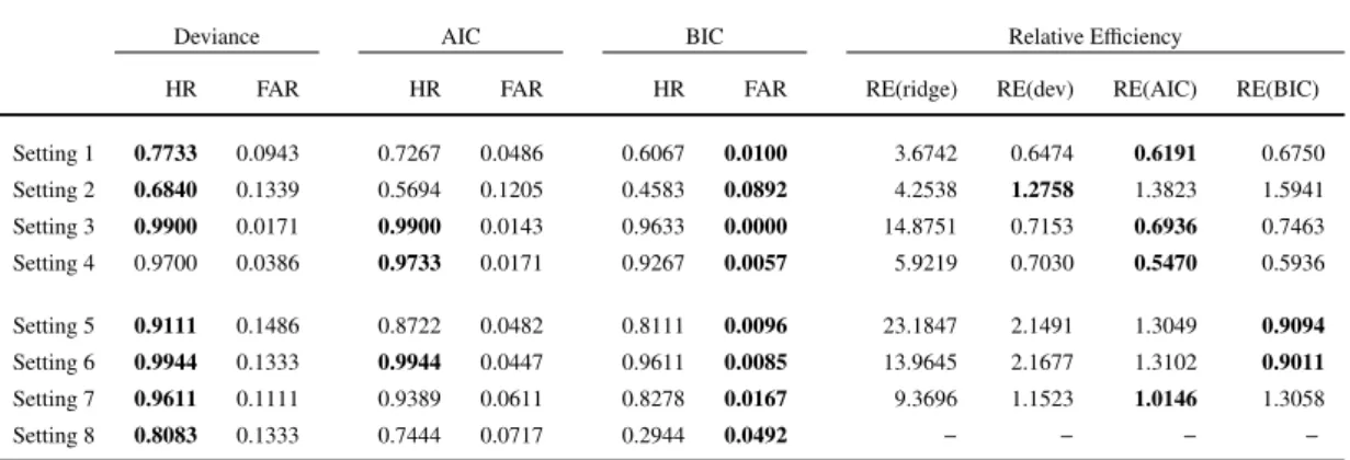
with all categorical predictors, these values are missing because MLE(oracle) estimates do not exist for any sample. The values with boldface represent the best result among the competitors in a particular setting. The deviance as a variable selection criterion is performing best for selecting the relevant covariates in almost all settings even when we have a small sample size relative to the number of covariates and with high correlations. AIC is a strong competitor of deviance than BIC and giving almost the same level of accuracy regarding the selection of the relevant predictors. In high dimensional setting when the model contains only binary or categorical predictors, hit rate with BIC as selection criteria is not so much appealing because it is ignoring most of the relevant predictors. But as for as the inclusion of non-relevant predictors is concerned, BIC is giving the best ”false alarm rate” in all situations. From the result of Table 2, AIC seems to be a good choice as criterion for variable selection when the both measures i.e., hit rate and false alarm rate for identification of the influential predictors are taken into account.
● ● ● ● ●● 2 4 6 8 log ( MSE ( β ^)) ● ● ● ● ● n=50, p=20, ρ =0.3 MLE(orac le) Boosting(de v) Boosting(AIC)Boosting(BIC) ssc−Ridg e 2 4 6 8 log ( MSE ( β ^)) ● ● ● ● ● n=50, p=20, ρ =0.7 MLE(orac le) Boosting(de v) Boosting(AIC)Boosting(BIC) ssc−Ridg e ● ● 2 4 6 8 log ( MSE ( β ^)) ● ● ● ● ● n=100, p=20, ρ =0.3 MLE(orac le) Boosting(de v) Boosting(AIC)Boosting(BIC) ssc−Ridg e ● ● ● 2 4 6 8 10 log ( MSE ( β ^)) ● ● ● ● ● n=100, p=20, ρ =0.7 MLE(orac le) Boosting(de v) Boosting(AIC)Boosting(BIC) ssc−Ridg e 6 7 8 9 log(MPE) ● ● ● ● ● n=50, p=20, ρ =0.3 MLE(orac le) Boosting(de v) Boosting(AIC)Boosting(BIC) ssc−Ridg e ● ● ● ● ● ● 5 6 7 8 log(MPE) ● ● ● ● ● n=50, p=20, ρ =0.7 MLE(orac le) Boosting(de v) Boosting(AIC)Boosting(BIC) ssc−Ridg e ● ● ● 4 5 6 7 8 log(MPE) ● ● ● ● ● n=100, p=20, ρ =0.3 MLE(orac le) Boosting(de v) Boosting(AIC)Boosting(BIC) ssc−Ridg e ● ● ● ● 4 5 6 7 8 log(MPE) ● ● ● ● ● n=100, p=20, ρ =0.7 MLE(orac le) Boosting(de v) Boosting(AIC)Boosting(BIC) ssc−Ridg e
Figure1:Illustration of the simulation study for first four settings without categorical covariates: Box plots for comparing
Boosting (using the criteria deviance, AIC and BIC) with MLE(oracle) and ssc-Ridge in terms of log(MSE(ˆβββ))(top panel)
and in terms of Mean Prediction Error i.e., log(MPE) (bottom panel). The solid circles within the boxes represent the mean of the data for which box plot is drawn.
● ● ● ● 2 4 6 8 log ( MSE ( β ^)) ● ● ● ● ● setting 5 MLE(orac le) Boosting(de v) Boosting(AIC)Boosting(BIC) ssc−Ridg e ● 1 2 3 4 5 6 7 8 log ( MSE ( β ^)) ● ● ● ● ● setting 6 MLE(orac le) Boosting(de v) Boosting(AIC)Boosting(BIC) ssc−Ridg e ● ● ● ● ● ● ● 4 5 6 7 log ( MSE ( β ^)) ● ● ● ● ● setting 7 MLE(orac le) Boosting(de v) Boosting(AIC)Boosting(BIC) ssc−Ridg e ● ● ● 6.9 7.0 7.1 7.2 log ( MSE ( β ^)) ● ● ● ● setting 8 MLE(orac le) Boosting(de v) Boosting(AIC)Boosting(BIC) ssc−Ridg e ● ● ● ● ● ● ● ● ● ● 5 6 7 8 log(MPE) ● ● ● ● ● setting 5 MLE(orac le) Boosting(de v) Boosting(AIC)Boosting(BIC) ssc−Ridg e ● ● ● ● ● ● 4 5 6 7 8 log(MPE) ● ● ● ● ● setting 6 MLE(orac le) Boosting(de v) Boosting(AIC)Boosting(BIC) ssc−Ridg e ● ● ● ● 6 7 8 9 log(MPE) ● ● ● ● ● setting 7 MLE(orac le) Boosting(de v) Boosting(AIC)Boosting(BIC) ssc−Ridg e 6.8 7.2 7.6 8.0 log(MPE) ● ● ● ● setting 8 MLE(orac le) Boosting(de v) Boosting(AIC)Boosting(BIC) ssc−Ridg e
Figure2:Illustration of the simulation study for high dimensional settings: Box plots for comparing Boosting (using the
criteria deviance, AIC and BIC) with MLE(oracle) and ssc-Ridge in terms of log(MSE(ˆβββ))(top panel) and in terms of
Mean Prediction Error i.e., log(MPE) (bottom panel). The solid circles within the boxes represent the mean of the data for which box plot is drawn.
T able 1: Comparison of Boosting approach with MLE(oracle) and ridge re gression with symmetric side constraint (ssc-Ridge) in terms of log(MSE( ˆ βββ )), de viance of the fit i.e., de viance( ˆ πππ )and Mean Prediction Error (MPE). The values with boldf ace represent the best result with a particular method among all competitors. log(MSE( ˆ βββ )) de viance( ˆ πππ ) MPE Boosting Boosting Boosting MLE de viance AIC BIC ssc-Ridge MLE de viance AIC BIC ssc-Ridge MLE de viance AIC BIC ssc-Ridge Setting 1 4 . 2276 4 . 2186 3 . 0089 2.9797 3 . 0325 28 . 9138 12 . 0440 11.7320 13 . 3471 39 . 1327 1022 . 3555 286 . 2253 278.3627 302 . 9525 1485 . 1743 Setting 2 5 . 6426 5 . 2404 5 . 2310 5 . 2795 5.0777 23 . 2785 12.5991 12 . 8019 16 . 0280 35 . 9622 612 . 9043 439.2145 472 . 5820 554 . 9007 1492 . 8805 Setting 3 2 . 8980 2 . 6479 2.5798 2 . 5915 5 . 6423 26 . 0146 15.7188 16 . 0922 18 . 0862 103 . 0675 229 . 9102 83 . 3936 80.6702 89 . 6679 1466 . 4339 Setting 4 4 . 5806 3 . 7675 3.5734 3 . 6326 5 . 3012 36 . 4438 25.1230 26 . 4086 28 . 9922 49 . 6566 378 . 0500 112 . 3644 90.5228 98 . 3068 821 . 2240 Setting 5 3 . 6859 3 . 8458 3 . 1852 2.6561 4 . 4734 33 . 1327 17 . 2544 13 . 3362 11.0415 119 . 1908 303 . 9448 231 . 7965 141 . 2749 104.9711 2544 . 0830 Setting 6 4 . 0363 3 . 8262 3 . 3816 2.9946 4 . 3078 53 . 9725 39 . 5517 30 . 7109 29.5848 184 . 2309 527 . 4985 525 . 9714 340 . 9851 258.2625 3433 . 4700 Setting 7 4.7309 5 . 5441 5 . 5521 5 . 5289 6 . 8844 159 . 6963 152 . 8985 154 . 5399 130.9688 552 . 0475 398 . 8496 314 . 6842 275.1543 352 . 9394 2495 . 1473 Setting 8 − 7 . 2015 7 . 2136 7.1781 6 . 9634 − 216 . 9942 235 . 3204 244 . 9447 96.7519 − 1073 . 2970 1043.7080 1348 . 9930 2462 . 4450 14
Table2: Hit rates (HR) and false alarm rates (FAR) for identifying the informative predictors when deviance, AIC and BIC are used as criteria for selecting a predictor in a boosting iteration. Deviance is used as stopping criterion with
10−fold cross-validation. Last four columns represent the relative efficiency (R.E.) of different approaches with respect
to MLE(oracle) in terms of Mean Prediction Error (MPE). A value less than one means that a particular approach is performing better than MLE(oracle). The boldface figures represent the best result among all competitor methods.
Deviance AIC BIC Relative Efficiency
HR FAR HR FAR HR FAR RE(ridge) RE(dev) RE(AIC) RE(BIC)
Setting 1 0.7733 0.0943 0.7267 0.0486 0.6067 0.0100 3.6742 0.6474 0.6191 0.6750 Setting 2 0.6840 0.1339 0.5694 0.1205 0.4583 0.0892 4.2538 1.2758 1.3823 1.5941 Setting 3 0.9900 0.0171 0.9900 0.0143 0.9633 0.0000 14.8751 0.7153 0.6936 0.7463 Setting 4 0.9700 0.0386 0.9733 0.0171 0.9267 0.0057 5.9219 0.7030 0.5470 0.5936 Setting 5 0.9111 0.1486 0.8722 0.0482 0.8111 0.0096 23.1847 2.1491 1.3049 0.9094 Setting 6 0.9944 0.1333 0.9944 0.0447 0.9611 0.0085 13.9645 2.1677 1.3102 0.9011 Setting 7 0.9611 0.1111 0.9389 0.0611 0.8278 0.0167 9.3696 1.1523 1.0146 1.3058 Setting 8 0.8083 0.1333 0.7444 0.0717 0.2944 0.0492 − − − −
5. Application
In this section two data sets are used to illustrate variable selection by use of themultinomBoostalgorithm and to show
how it differs from the Lasso approach which focuses on parameter selection rather than variable selection. Both of
the data sets are taken from the UCI machine learning repository.
5.1. Glass Identification Data
The first data set concerns the identification of type of glass (Blake et al. (1998)). The data comprises 214 observa-tions. The response variable is the type of glass with six response categories given as: BFP (building windows float processed), BFNP (building windows non float processed), VFP (vehicle windows float processed), Con (containers), TW (tableware) and HL (headlamps). The nine continuously valued covariates are RI (refractive index), Na (Sodium), Mg (Magnesium), Al (Aluminum), Si (Silicon), K (potassium), Ca (calcium), Ba (Barium) and Fe (iron). The unit of measurement for all covariates other than refractive index is the weight percent in corresponding oxide.
For the identification of influential covariates, themultinomBoostalgorithm is used. Three measures i.e., deviance,
AIC and BIC are used to select a variable for updating in a boosting iteration. With all these three criteria, while
using 10−fold cross-validation for deciding the optimal number of boosting iterations, only three covariates i.e., Na,
Mg and Al are identified as potential covariates whereas the rest of the covariates are found non-informative with zero parameter estimates for all six response categories. The same data set is also analyzed by using the lasso approach.
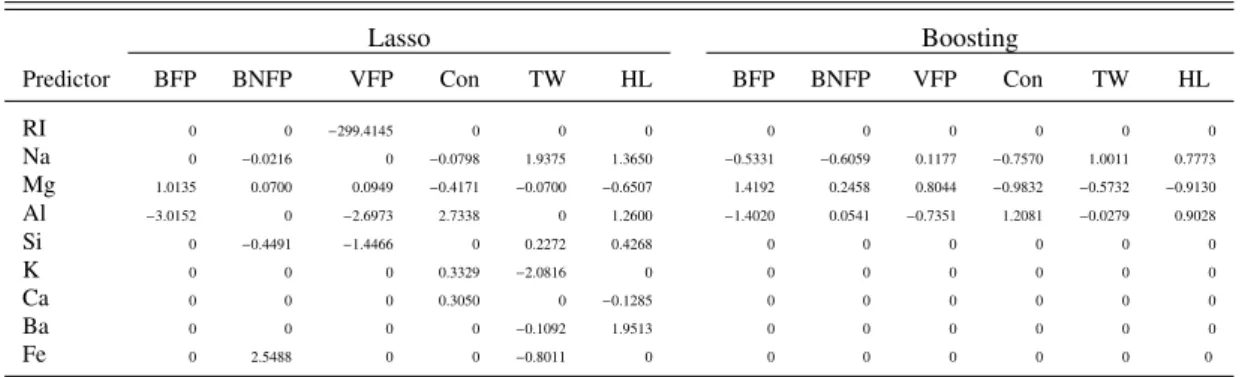
Table3: Parameter estimates for six categories of ”Type of Glass” with Lasso approach and the multinomBoost. For
the boosting estimates AIC is used for variable selection and deviance is used as stopping criterion based on10−fold
cross-validation.
Lasso Boosting
Predictor BFP BNFP VFP Con TW HL BFP BNFP VFP Con TW HL
RI 0 0 −299.4145 0 0 0 0 0 0 0 0 0 Na 0 −0.0216 0 −0.0798 1.9375 1.3650 −0.5331 −0.6059 0.1177 −0.7570 1.0011 0.7773 Mg 1.0135 0.0700 0.0949 −0.4171 −0.0700 −0.6507 1.4192 0.2458 0.8044 −0.9832 −0.5732 −0.9130 Al −3.0152 0 −2.6973 2.7338 0 1.2600 −1.4020 0.0541 −0.7351 1.2081 −0.0279 0.9028 Si 0 −0.4491 −1.4466 0 0.2272 0.4268 0 0 0 0 0 0 K 0 0 0 0.3329 −2.0816 0 0 0 0 0 0 0 Ca 0 0 0 0.3050 0 −0.1285 0 0 0 0 0 0 Ba 0 0 0 0 −0.1092 1.9513 0 0 0 0 0 0 Fe 0 2.5488 0 0 −0.8011 0 0 0 0 0 0 0
the basis of 10−fold cross validation was 0.009993293.The parameter estimates for lasso approach using this penalty
term along with those from the boosting approach with AIC as variable selection criterion and deviance based on
10−fold cross-validation as stopping criterion are given in Table 3. The results in Table 3 show that the lasso approach
does parameter selection but not variable selection. With lasso, all predictors are found relevant because at least one estimate for some response category is non-zero for each predictor. The boosting approach suggests only three predictors as relevant and the rest of the predictors as non-informative. In contrast to lasso, the boosting approach is selecting (or ignoring) the whole block of category-specific parameter estimates for each predictor with non-zero (or
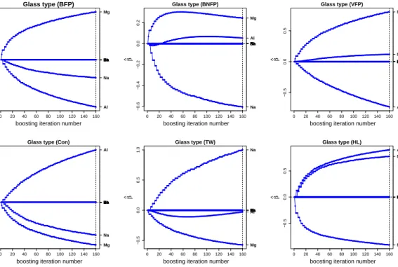
zero) values of the parameter estimates for all response categories. The coefficients build-up for relevant predictors for
each response category resulting from boosting are plotted in Figure 3. The names of all non-informative predictors
are overlapped against zero value on the right side of each plot. Figure 3 is showing the coefficients build-up only
for the informative covariates because the multinomBoostalgorithm sets parameter estimates to zero for all those
predictors which fulfill the criteria given in (10) at final boosting iteration.
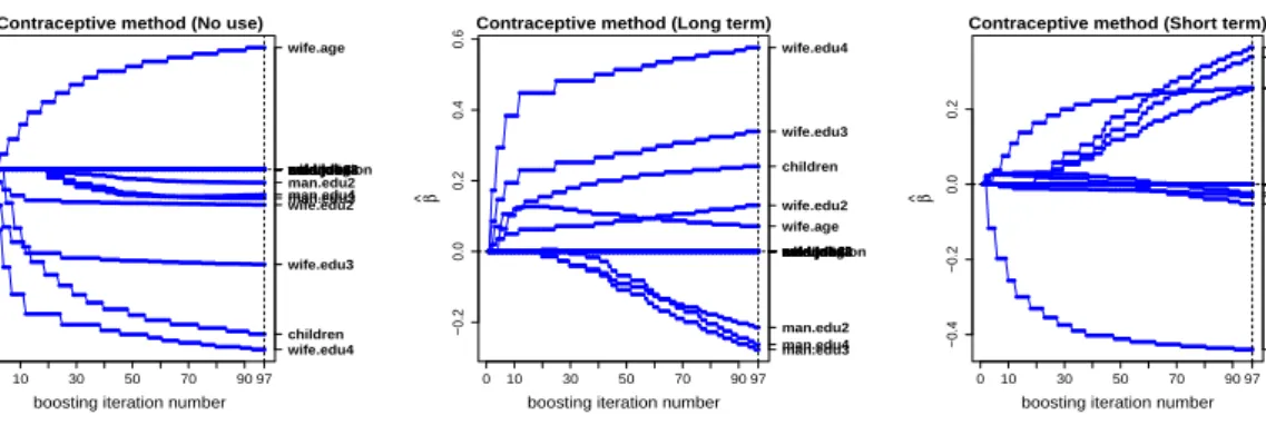
5.2. Contraceptive Method Choice Data
The second data set considered provided by Lim et al. (2000) is a subset of the 1987 National Indonesia Contraceptive Prevalence Survey. The sample, 1473 married women who were either not pregnant or did not know if they were at the time of interview. The problem is to analyse the current contraceptive method choice (no use, long-term methods, or short-term methods) of a woman based on 10 demographic and socio-economic characteristics as: Wife’s age , Wife’s
education (wife.edu; 1=low, 2, 3, 4=high), Husband’s education (husband.edu; 1=low, 2, 3, 4=high), Number of
children ever born, Wife’s religion (0 =Non-Islam, 1 =Islam), Wife’s now working? (0 =Yes, 1 =No), Husband’s
occupation (categorical: 1,2,3,4), standard of living (sol.index; 1=low, 2, 3, 4=high) and media exposure (0=Good,
1=Not good).
For this data set, we used the deviance for variable selection among the candidate predictors. For large samples using 16
●●●●●●●●●●●●●●●●●●●●●●●●●●●●●●●●●●●●●●●●●●●●●●●●●●●●●●●●●●●●●●●●●●●●●●●●●●●●●●●●●●●●●●●●●●●●●●●●●●●●●●●●●●●●●●●●●●●●●●●●●●●●●●●●●●●●●●●●●●●●●●●●●●●●●●●●●●●●●●●● −1.5 −1.0 −0.5 0.0 0.5 1.0 1.5 Glass type (BFP)
boosting iteration number
β ^ ●●●●●●●●●●●●●●●●●●●●●●●●●●●●●●●●●●●●●●●●●●●●●●●●●●●●●●●●●●●●●●●●●●●●●●●●●●●●●●●●●●●●●●●●●●●●●●●●●●●●●●●●●●●●●●●●●●●●●●●●●●●●●●●●●●●●●●●●●●●●●●●●●●●●●●●●●●●●●●●● ● ● ●●●● ●●● ●●●●● ●●●●●●●●●● ●●●●●●●●●● ●●●●●●●●●●●●●● ●●●●●●●●●●●●●●●●●●●●●●●●●●●●●●●●●●●●●●●●●●●●●●●●●●●●●●●●●●●●●●●●●●●●●●●●●●●●●●●●●●●●●●●●●●●●●●●●●●●●●●●●●●●●●●●● ●●● ●●●● ●●● ●●● ●●● ●●●●●●●●●● ●●●●●●● ●●●●●●●●●● ●●●●●●●●●● ●●●●●●●●●●●●●●●●●●●●●●●●●●●●●●●●●●●●●●●●●●●●●●●●●●●●●●●●●●●●●●●●●●●●●●●●●●●●●●●●●●●●●●●●●●●●●●●●●●●●●●●●●●● ●●●●●●●●●●●●●●●●●●●●●●●●●●●●●●●●●●●●●●●●●●●●●●●●●●●●●●●●●●●●●●●●●●●●●●●●●●●●●●●●●●●●●●●●●●●●●●●●●●●●●●●●●●●●●●●●●●●●●●●●●●●●●●●●●●●●●●●●●●●●●●●●●●●●●●●●●●●●●●●● ●●●●●●●●●●●●●●●●●●●●●●●●●●●●●●●●●●●●●●●●●●●●●●●●●●●●●●●●●●●●●●●●●●●●●●●●●●●●●●●●●●●●●●●●●●●●●●●●●●●●●●●●●●●●●●●●●●●●●●●●●●●●●●●●●●●●●●●●●●●●●●●●●●●●●●●●●●●●●●●● ●●●●●●●●●●●●●●●●●●●●●●●●●●●●●●●●●●●●●●●●●●●●●●●●●●●●●●●●●●●●●●●●●●●●●●●●●●●●●●●●●●●●●●●●●●●●●●●●●●●●●●●●●●●●●●●●●●●●●●●●●●●●●●●●●●●●●●●●●●●●●●●●●●●●●●●●●●●●●●●● ●●●●●●●●●●●●●●●●●●●●●●●●●●●●●●●●●●●●●●●●●●●●●●●●●●●●●●●●●●●●●●●●●●●●●●●●●●●●●●●●●●●●●●●●●●●●●●●●●●●●●●●●●●●●●●●●●●●●●●●●●●●●●●●●●●●●●●●●●●●●●●●●●●●●●●●●●●●●●●●● ●●●●●●●●●●●●●●●●●●●●●●●●●●●●●●●●●●●●●●●●●●●●●●●●●●●●●●●●●●●●●●●●●●●●●●●●●●●●●●●●●●●●●●●●●●●●●●●●●●●●●●●●●●●●●●●●●●●●●●●●●●●●●●●●●●●●●●●●●●●●●●●●●●●●●●●●●●●●●●●● 0 20 40 60 80 100 120 140 160 Al Na RI Ca Si K Ba Fe Mg ● ●●●●●●●●●●●●●●●●●●●●●●●●●●●●●●●●●●●●●●●●●●●●●●●●●●●●●●●●●●●●●●●●●●●●●●●●●●●●●●●●●●●●●●●●●●●●●●●●●●●●●●●●●●●●●●●●●●●●●●●●●●●●●●●●●●●●●●●●●●●●●●●●●●●●●●●●●●●●●●● −0.6 −0.4 −0.2 0.0 0.2 Glass type (BNFP)
boosting iteration number
β ^ ● ●●●● ●●● ●●●● ●●● ●●● ●●● ●●●● ●●●● ●●● ●●●●●●●●●●●●●●●●●●●●●●●●●● ●●●●●●●●● ● ●●●●●●●●●●●●●●●●●●●●●●●●●●●●●●●●●●●●●●●●●●●●●●●●●●●●●●●●●●●●●●●●●●●●●●●●●●●●●●●●●●●●●●●●●●●● ● ● ●●●● ●●● ●● ●●●●●●●●● ● ●●●●●●●●●●●●●●●●●●●●●●●●●●●●●●●●●●●●●●●●●●●●●●●●●●●●●●●●●●●●●●●●●●●●●●●●●●●●●●●●●●●●●●●●●●●●●●●●●●●●●●●●●●●●●●●●●●●●●●●●●●●●●●●●●●●●●●●●●●● ● ●●●●●●●●●●●●●●●●●●●●●●●●●●●●●●●●●●●●●●●●●●●●●●●●●●●●●●●●●●●●●●●●●●●●●●●●●●●●●●●●●●●●●●●●●●●●●●●●●●●●●●●●●●●●●●●●●●●●●●●●●●●●●●●●●●●●●●●●●●●●●●●●●●●●●●●●●●●●●●● ● ●●●●●●●●●●●●●●●●●●●●●●●●●●●●●●●●●●●●●●●●●●●●●●●●●●●●●●●●●●●●●●●●●●●●●●●●●●●●●●●●●●●●●●●●●●●●●●●●●●●●●●●●●●●●●●●●●●●●●●●●●●●●●●●●●●●●●●●●●●●●●●●●●●●●●●●●●●●●●●● ● ●●●●●●●●●●●●●●●●●●●●●●●●●●●●●●●●●●●●●●●●●●●●●●●●●●●●●●●●●●●●●●●●●●●●●●●●●●●●●●●●●●●●●●●●●●●●●●●●●●●●●●●●●●●●●●●●●●●●●●●●●●●●●●●●●●●●●●●●●●●●●●●●●●●●●●●●●●●●●●● ● ●●●●●●●●●●●●●●●●●●●●●●●●●●●●●●●●●●●●●●●●●●●●●●●●●●●●●●●●●●●●●●●●●●●●●●●●●●●●●●●●●●●●●●●●●●●●●●●●●●●●●●●●●●●●●●●●●●●●●●●●●●●●●●●●●●●●●●●●●●●●●●●●●●●●●●●●●●●●●●● ● ●●●●●●●●●●●●●●●●●●●●●●●●●●●●●●●●●●●●●●●●●●●●●●●●●●●●●●●●●●●●●●●●●●●●●●●●●●●●●●●●●●●●●●●●●●●●●●●●●●●●●●●●●●●●●●●●●●●●●●●●●●●●●●●●●●●●●●●●●●●●●●●●●●●●●●●●●●●●●●● ● ●●●●●●●●●●●●●●●●●●●●●●●●●●●●●●●●●●●●●●●●●●●●●●●●●●●●●●●●●●●●●●●●●●●●●●●●●●●●●●●●●●●●●●●●●●●●●●●●●●●●●●●●●●●●●●●●●●●●●●●●●●●●●●●●●●●●●●●●●●●●●●●●●●●●●●●●●●●●●●● 0 20 40 60 80 100 120 140 160 Na RI Ca Ba Si K Fe Al Mg ●●●●●●●●●●●●●●●●●●●●●●●●●●●●●●●●●●●●●●●●●●●●●●●●●●●●●●●●●●●●●●●●●●●●●●●●●●●●●●●●●●●●●●●●●●●●●●●●●●●●●●●●●●●●●●●●●●●●●●●●●●●●●●●●●●●●●●●●●●●●●●●●●●●●●●●●●●●●●●●● −0.5 0.0 0.5 Glass type (VFP)
boosting iteration number
β ^ ●●●●●●●●●●●●●●●●●●●●●●●●●●●●●●●●●●●●●●●●●●●●●●●●●●●●●●●●●●●●●●●●●●●●●●●●●●●●●●●●●●●●●●●●●●●●●●●●●●●●●●●●●●●●●●●●●●●●●●●●●●●●●●●●●●●●●●●●●●●●●●●●●●●●●●●●●●●●●●●● ● ● ● ●●●●●● ● ●●●● ●●●●●●●●●● ●●●●●● ●●●●●●●●●●●●●●●●●●●●●●●●●●●●●●●●●●●●●●●●●●●●●●●●●●●●●●●●●●●●●●●●●●●●●●●●●●●●●●●●●●●●●●●●●●●●●●●●●●●●●●●●●●●●●●●●●●●●●●●●●●●●●●●●●● ●●● ●●●● ●●●●●● ●●●●●●●●●●●●●●●●●●●●●●●●●●● ●●●●●●●●●●●●●●●●●●●●●●●●●●●●●●●●●●● ● ●●●●●●● ●●●●●●●●●●●●●●●●●●●●●●●●●●● ●●●●●●●●●●●●●●●●●●●● ●●●●●●●●●●●●●●●●●●●●●●●●●●●●●● ●●●●●●●●●●●●●●●●●●●●●●●●●●●●●●●●●●●●●●●●●●●●●●●●●●●●●●●●●●●●●●●●●●●●●●●●●●●●●●●●●●●●●●●●●●●●●●●●●●●●●●●●●●●●●●●●●●●●●●●●●●●●●●●●●●●●●●●●●●●●●●●●●●●●●●●●●●●●●●●● ●●●●●●●●●●●●●●●●●●●●●●●●●●●●●●●●●●●●●●●●●●●●●●●●●●●●●●●●●●●●●●●●●●●●●●●●●●●●●●●●●●●●●●●●●●●●●●●●●●●●●●●●●●●●●●●●●●●●●●●●●●●●●●●●●●●●●●●●●●●●●●●●●●●●●●●●●●●●●●●● ●●●●●●●●●●●●●●●●●●●●●●●●●●●●●●●●●●●●●●●●●●●●●●●●●●●●●●●●●●●●●●●●●●●●●●●●●●●●●●●●●●●●●●●●●●●●●●●●●●●●●●●●●●●●●●●●●●●●●●●●●●●●●●●●●●●●●●●●●●●●●●●●●●●●●●●●●●●●●●●● ●●●●●●●●●●●●●●●●●●●●●●●●●●●●●●●●●●●●●●●●●●●●●●●●●●●●●●●●●●●●●●●●●●●●●●●●●●●●●●●●●●●●●●●●●●●●●●●●●●●●●●●●●●●●●●●●●●●●●●●●●●●●●●●●●●●●●●●●●●●●●●●●●●●●●●●●●●●●●●●● ●●●●●●●●●●●●●●●●●●●●●●●●●●●●●●●●●●●●●●●●●●●●●●●●●●●●●●●●●●●●●●●●●●●●●●●●●●●●●●●●●●●●●●●●●●●●●●●●●●●●●●●●●●●●●●●●●●●●●●●●●●●●●●●●●●●●●●●●●●●●●●●●●●●●●●●●●●●●●●●● 0 20 40 60 80 100 120 140 160 Al RI K Ca Si Ba Fe Na Mg ●●●●●●●●●●●●●●●●●●●●●●●●●●●●●●●●●●●●●●●●●●●●●●●●●●●●●●●●●●●●●●●●●●●●●●●●●●●●●●●●●●●●●●●●●●●●●●●●●●●●●●●●●●●●●●●●●●●●●●●●●●●●●●●●●●●●●●●●●●●●●●●●●●●●●●●●●●●●●●●● −1.0 −0.5 0.0 0.5 1.0
Glass type (Con)
boosting iteration number
β ^ ●●●●●●●● ●●●● ● ●●●●●●●●●●●●●●●●●●●●●●●●●●●●●●●●●●●●●●●●●●●●●●●●●●●●●●●●●●●●●●●●●●●●●●●●●●●●●●●●●●●●●●●●●●●●●●●●●●●●●●●●●●●●●●●●●●●●●●●●●●●●●●●●●●●●●●●●●●●●●●●●●●● ● ● ●●●● ●●● ●● ●●● ●●●●●●●●●● ●●●●●●●●●●●●●●●●●●●● ●●●●●●●●●●●●●●●●●●●●●●●●●●●●●●●●●●●●●●●●●●●●●●●●●●●●●●●●●●●●●●●●●●●●●●●●●●●●●●●●●●●●●●●●●●●●●●●●●●●●●●●●●●●●●●●●●●●● ●●● ●●●●●●● ●●●●●● ●●●●●●●●●● ●●●●●●●●●●●●●●●●●●●●●●●●●●●●●●●●● ●●●●●●●●●●●●●● ●●●●●●●●●●●●● ●●●●●●●●●●●●●●●●●●●● ●●●●●●●●●●●●●●●●●●●●●●●●●●●●●●●●●●●●●●●● ●●●●●●●●●●●●●● ●●●●●●●●●●●●●●●●●●●●●●●●●●●●●●●●●●●●●●●●●●●●●●●●●●●●●●●●●●●●●●●●●●●●●●●●●●●●●●●●●●●●●●●●●●●●●●●●●●●●●●●●●●●●●●●●●●●●●●●●●●●●●●●●●●●●●●●●●●●●●●●●●●●●●●●●●●●●●●●● ●●●●●●●●●●●●●●●●●●●●●●●●●●●●●●●●●●●●●●●●●●●●●●●●●●●●●●●●●●●●●●●●●●●●●●●●●●●●●●●●●●●●●●●●●●●●●●●●●●●●●●●●●●●●●●●●●●●●●●●●●●●●●●●●●●●●●●●●●●●●●●●●●●●●●●●●●●●●●●●● ●●●●●●●●●●●●●●●●●●●●●●●●●●●●●●●●●●●●●●●●●●●●●●●●●●●●●●●●●●●●●●●●●●●●●●●●●●●●●●●●●●●●●●●●●●●●●●●●●●●●●●●●●●●●●●●●●●●●●●●●●●●●●●●●●●●●●●●●●●●●●●●●●●●●●●●●●●●●●●●● ●●●●●●●●●●●●●●●●●●●●●●●●●●●●●●●●●●●●●●●●●●●●●●●●●●●●●●●●●●●●●●●●●●●●●●●●●●●●●●●●●●●●●●●●●●●●●●●●●●●●●●●●●●●●●●●●●●●●●●●●●●●●●●●●●●●●●●●●●●●●●●●●●●●●●●●●●●●●●●●● ●●●●●●●●●●●●●●●●●●●●●●●●●●●●●●●●●●●●●●●●●●●●●●●●●●●●●●●●●●●●●●●●●●●●●●●●●●●●●●●●●●●●●●●●●●●●●●●●●●●●●●●●●●●●●●●●●●●●●●●●●●●●●●●●●●●●●●●●●●●●●●●●●●●●●●●●●●●●●●●● 0 20 40 60 80 100 120 140 160 Mg Na RI Ba Si K Ca Fe Al ● ●●●●●●●●●●●●●●●●●●●●●●●●●●●●●●●●●●●●●●●●●●●●●●●●●●●●●●●●●●●●●●●●●●●●●●●●●●●●●●●●●●●●●●●●●●●●●●●●●●●●●●●●●●●●●●●●●●●●●●●●●●●●●●●●●●●●●●●●●●●●●●●●●●●●●●●●●●●●●●● −0.5 0.0 0.5 1.0 Glass type (TW)
boosting iteration number
β ^ ● ●●●● ●●● ●●●● ●●● ●●● ●●●●●●● ●●●●●●● ●●●●●●● ●●●●●●● ●●●●●●●●●●●●●●●●●●●●●●●●●●●●●●●●●●●●●●●●●●●●●●●● ●●●●●●●●●●●●●●●●●●●●●●● ●●●●●●●●●●●●●●●●●●●●●●●●●●●●●●●●●●●●●●●●●●● ● ● ●●●●●●● ●●●●●●●●●●●●●●●●●●●●●●●●●●●●●●●● ●●●●●●●●●●●●●●●●●●●●●●●●●●●●●●●●●●●●●●●●●●●●●●●●●●●●●●●●●●●●●●●●●●●●●●●●●●●●●●●●●●●●●●●●●●●●●●●●●●●●●●●●●●●●●●●●●●●●●●● ● ●●●●●●●●●●●●●●●●●●●●●●●●●●●●●●●●●●●●●●●●●●●●●●●●●●●●●●●●●●●●●●●●●●●●●●●●●●●●●●●●●●●●●●●●●●●●●●●●●●●●●●●●●●●●●●●●●●●●●●●●●●●●●●●●●●●●●●●●●●●●●●●●●●●●●●●●●●●●●●● ● ●●●●●●●●●●●●●●●●●●●●●●●●●●●●●●●●●●●●●●●●●●●●●●●●●●●●●●●●●●●●●●●●●●●●●●●●●●●●●●●●●●●●●●●●●●●●●●●●●●●●●●●●●●●●●●●●●●●●●●●●●●●●●●●●●●●●●●●●●●●●●●●●●●●●●●●●●●●●●●● ● ●●●●●●●●●●●●●●●●●●●●●●●●●●●●●●●●●●●●●●●●●●●●●●●●●●●●●●●●●●●●●●●●●●●●●●●●●●●●●●●●●●●●●●●●●●●●●●●●●●●●●●●●●●●●●●●●●●●●●●●●●●●●●●●●●●●●●●●●●●●●●●●●●●●●●●●●●●●●●●● ● ●●●●●●●●●●●●●●●●●●●●●●●●●●●●●●●●●●●●●●●●●●●●●●●●●●●●●●●●●●●●●●●●●●●●●●●●●●●●●●●●●●●●●●●●●●●●●●●●●●●●●●●●●●●●●●●●●●●●●●●●●●●●●●●●●●●●●●●●●●●●●●●●●●●●●●●●●●●●●●● ● ●●●●●●●●●●●●●●●●●●●●●●●●●●●●●●●●●●●●●●●●●●●●●●●●●●●●●●●●●●●●●●●●●●●●●●●●●●●●●●●●●●●●●●●●●●●●●●●●●●●●●●●●●●●●●●●●●●●●●●●●●●●●●●●●●●●●●●●●●●●●●●●●●●●●●●●●●●●●●●● ● ●●●●●●●●●●●●●●●●●●●●●●●●●●●●●●●●●●●●●●●●●●●●●●●●●●●●●●●●●●●●●●●●●●●●●●●●●●●●●●●●●●●●●●●●●●●●●●●●●●●●●●●●●●●●●●●●●●●●●●●●●●●●●●●●●●●●●●●●●●●●●●●●●●●●●●●●●●●●●●● 0 20 40 60 80 100 120 140 160 Mg Al RI K Si Ca Ba Fe Na ●●●●●●●●●●●●●●●●●●●●●●●●●●●●●●●●●●●●●●●●●●●●●●●●●●●●●●●●●●●●●●●●●●●●●●●●●●●●●●●●●●●●●●●●●●●●●●●●●●●●●●●●●●●●●●●●●●●●●●●●●●●●●●●●●●●●●●●●●●●●●●●●●●●●●●●●●●●●●●●● −0.5 0.0 0.5 Glass type (HL)
boosting iteration number
β ^ ●●●●● ●●● ●●●● ●●● ● ●●●●● ●●●●●●●● ● ●●●●●●●●●●●● ● ●●●●●●●●●●●●● ●●●●●●●●●●●●●●●●●●●●●●●●●●●●●●●●●●●●●●●●●●●●●●●●●●●●●●●●●●●●●●●●●●●●●●●●●●●●●●●●●●●●●●●●●●●●●●●●●●●●●●●● ● ● ● ●●● ●●● ● ● ●●● ●●● ●●●●●●●●●●●●●●●●●●●●●●●●●●●●●●●●●●●●●●●●●●●●●●●●●●●●●●●●●●●●●●●●●●●●●●●●●●●●●●●●●●●●●●●●●●●●●●●●●●●●●●●●●●●●●●●●●●●●●●●●●●●●●●●●●●●●●●●●●●●●●●● ●●● ●●●● ●●● ●●● ●●●●●● ●●●●●●● ●●●●●●●●●●● ●●●●●●●●●●●●●●●●●●●●●●●●●● ●●●●●●●●●●●●●●●●●●●●●●●●●●●●●●●●●●●●●●●●●●●●●●●●●●●●●●●●●●●●●●●●●●●●●●●●●●●●●●●●●●●●●●●●●●●●●●●●● ●●●●●●●●●●●●●●●●●●●●●●●●●●●●●●●●●●●●●●●●●●●●●●●●●●●●●●●●●●●●●●●●●●●●●●●●●●●●●●●●●●●●●●●●●●●●●●●●●●●●●●●●●●●●●●●●●●●●●●●●●●●●●●●●●●●●●●●●●●●●●●●●●●●●●●●●●●●●●●●● ●●●●●●●●●●●●●●●●●●●●●●●●●●●●●●●●●●●●●●●●●●●●●●●●●●●●●●●●●●●●●●●●●●●●●●●●●●●●●●●●●●●●●●●●●●●●●●●●●●●●●●●●●●●●●●●●●●●●●●●●●●●●●●●●●●●●●●●●●●●●●●●●●●●●●●●●●●●●●●●● ●●●●●●●●●●●●●●●●●●●●●●●●●●●●●●●●●●●●●●●●●●●●●●●●●●●●●●●●●●●●●●●●●●●●●●●●●●●●●●●●●●●●●●●●●●●●●●●●●●●●●●●●●●●●●●●●●●●●●●●●●●●●●●●●●●●●●●●●●●●●●●●●●●●●●●●●●●●●●●●● ●●●●●●●●●●●●●●●●●●●●●●●●●●●●●●●●●●●●●●●●●●●●●●●●●●●●●●●●●●●●●●●●●●●●●●●●●●●●●●●●●●●●●●●●●●●●●●●●●●●●●●●●●●●●●●●●●●●●●●●●●●●●●●●●●●●●●●●●●●●●●●●●●●●●●●●●●●●●●●●● ●●●●●●●●●●●●●●●●●●●●●●●●●●●●●●●●●●●●●●●●●●●●●●●●●●●●●●●●●●●●●●●●●●●●●●●●●●●●●●●●●●●●●●●●●●●●●●●●●●●●●●●●●●●●●●●●●●●●●●●●●●●●●●●●●●●●●●●●●●●●●●●●●●●●●●●●●●●●●●●● 0 20 40 60 80 100 120 140 160 Mg RI K Ba Si Ca Fe Na Al
Figure3:Coefficient build-up in boosting for ”Type of glass” data. The vertical dotted line represents the optimal boosting
iteration number decided on the basis of10−fold cross-validation when deviance is used as a stopping criterion. AIC is
used for predictor selection. The names of all non-informative predictors are overlapped against zero value on the right side of each plot.
AIC or BIC as variable selection criterion increases the computational burden and can slow the algorithm because of computation of hat matrix at each boosting iteration for each of the candidate predictors. The optimal number of
boosting iterations was decided by deviance with 10−fold cross-validation. For computation of lasso estimates again
theglmnetpackage (Friedman et al. (2010)) of R was used. The optimal value of penalty term decided with 10−fold
cross-validation was 0.001016358.The lasso estimates with this penalty are given in Table 4 along with corresponding
boosting estimates. As in Section 5.1, again the difference between parameter selection (by lasso approach) and
variable selection (boosting approach) becomes obvious from Table 4. Here the process is one step more complex in the sense that categorical covariates are included. So with variable selection all parameters associated with dummies of the categorical covariate for all response categories should be selected or rejected at the same time. From the results of Table 4 it is clear that the boosting approach is following that rule but lasso is not. Once again with the lasso approach all the variables are found relevant when at least one predictor (or dummy associated with the categorical predictor) had non-zero estimate(s) for at least one response category. In contrast boosting is recommending just four informative predictors by selecting all of the parameters associated with the predictors for all response categories. The informative covariates include two continuous predictors i.e., wife’s age and number of children ever born, and two