HAL Id: halshs-02418950
https://halshs.archives-ouvertes.fr/halshs-02418950
Submitted on 20 Dec 2019
HAL
is a multi-disciplinary open access
archive for the deposit and dissemination of
sci-entific research documents, whether they are
pub-lished or not. The documents may come from
teaching and research institutions in France or
L’archive ouverte pluridisciplinaire
HAL
, est
destinée au dépôt et à la diffusion de documents
scientifiques de niveau recherche, publiés ou non,
émanant des établissements d’enseignement et de
recherche français ou étrangers, des laboratoires
Dynamic Frailty Count Process in Insurance: A Unified
Framework for Estimation, Pricing, and Forecasting
Yang Lu
To cite this version:
Yang Lu.
Dynamic Frailty Count Process in Insurance: A Unified Framework for Estimation,
Pricing, and Forecasting.
Journal of Risk and Insurance, Wiley, 2018, 85 (4), pp.1083-1102.
�10.1111/jori.12190�. �halshs-02418950�
Dynamic Frailty Count Process in Insurance: A Unified
Framework for Estimation, Pricing and Forecasting
Yang Lu (Aix-Marseille University)
September 14, 2016
forthcoming,Journal of Risk and Insurance
Abstract
We study count processes in insurance, in which the underlying risk factor is time-varying and unobservable. The factor follows an autoregressive gamma process, and the resulting model generalizes the static Poisson-Gamma model and allows for closed form expression for the posterior Bayes (linear or non-linear) premium. Moreover the estimation and forecasting can be conducted within the same framework in a rather efficient way. An example of automobile insurance pricing illustrates the ability of the model to capture the duration-dependent, non-linear impact of past claims on future ones and the improvement of the Bayes pricing method compared to the linear credibility approach.
Key words: stochastic intensity (dynamic frailty) count process, affine process, non-linear pricing/forecasting, bonus-malus.
AcknowledgementI thank Christian Gourieroux, as well as two anonymous referees for insightful comments that greatly improved the presentation of the paper.
1
Introduction
We propose a time series model for count variables encountered in Insurance, when the underlying risk factor is time-varying and unobservable. We introduce the autoregressive gamma process for the latent factor dynamics, and show how it provides an integrated framework for the efficient estimation, pricing and forecasting of the risk. One typical application of the model is automobile insurance, for which the insurer holds the history of individual yearly claim counts over several periods. This information should then be taken into account in order to update the future premium regularly, on an individual basis.
Ideally, this latter exercise, also called posterior pricing, should be conducted via the Bayes rule. However, very often, due to the lack of analytic expression of the Bayes premium for most models, the linear credibility method is employed to get an approximation. This practice has some drawbacks. Indeed, the credibility framework is solely based on the first two moments of the count process1 and does not fully capture the dynamics of the latter, which is clearly
non-Gaussian. Thus the linear premium approach induces a systematic pricing bias which has to be evaluated. More importantly, the mean-variance credibility approach is not adapted for a complete risk, which includes non-linear pricing/forecasting, or simulation of the future trajectory of the count process.
In a pioneering work, Dionne and Vanasse (1989) propose a Poisson-Gamma (i.e. negative binomial) model. They show that in a Poisson model with Gamma distributed individual random effect (or frailty, or unobserved heterogeneity), the Bayes premium is linear in past observations and thus can be obtained in closed form. However, one shortcoming of this approach is that all the past observations have the same weight in the premium updating formula, or equivalently, the random effect is time-invariant. There is a growing interest on models that improve this feature [see e.g. Sundt (1988); Brouhns et al. (2003); Purcaru and Denuit (2003); Abdallah et al. (2016); Le Courtois (2015)]. In particular, Pinquet et al. (2001) generalize the negative binomial model by replacing the static frailty with a dynamic one and empirically found evidence of serial correlation of the individual frailty. However, the model suffers from classical computational burdens of models with dynamic unobserved factors, and the only linear credibility premium is available.
Our paper contributes to this literature by proposing a new dynamic frailty model. The static gamma frailty is replaced by a dynamic process with Gamma marginal distribution, called autoregressive gamma process (ARG), which generalizes Dionne and Vanasse (1989)’s model. It belongs to the so-called affine, or compound autoregressive family [see Darolles et al. (2006)]. We show that it provides a tractable, unified approach for estimation, linear or non-linear pricing,
as well as forecasting. More precisely, first, its estimation does not require simulation-based techniques. Second, we show that the exact Bayesian forecast formula allows for a closed form expression. Third, this model can be easily extended to higher dimensions, when multiple-risk policies are introduced. We then illustrate the advantage of this new approach via an example of pricing. In particular we show that how the model successfully captures the non-linear, and duration-dependence, and how the credibiilty premium induces a pricing bias with respect to the Bayes premium.
On the contrary to the state-space based, or parameter-driven model, the usual count pro-cess literature [see e.g. Harvey and Fernandes (1989); Frees and Wang (2005); Gourieroux and Jasiak (2004); Bolanc´e et al. (2007); Abdallah et al. (2016)] isobservation-driven, i.e., it specifies directly the dynamics of the observable count variables without serially correlated latent factor. The advantage of parameter-driven models is that it provides a more intuitive interpretation in terms of omitted pricing factors, and can better capture some key features of the observable count data, such as non-linear serial dependence and over-dispersion [see also Davis et al. (2003) for a discussion]. Nevertheless, while state-space models are popular in Finance2, they have
enjoyed a limited success in Insurance. Clearly, one of the reasons is the computational burden involved, since the Bayesian simulation methods typically employed for financial time series are too cumbersome for panel count data3. Our paper solves the computational burden by proposing the ARG specification and deriving the exact predictive formulas.
The rest of the paper is organized as follows. Section 2 reviews briefly the negative binomial model and motivates the dynamic frailty framework. Section 3 introduces our model with au-toregressive gamma (ARG) based dynamic frailty. We first review the basic properties of this process, and then show how the estimation, Bayes premium updating, as well as non-linear fore-casting issues are all rendered easy within the same framework. Section 4 provides a numerical illustration in terms of pricing. Section 5 briefly discusses the prospective bivariate extension of the model. Section 6 concludes. Proofs are gathered in an online Appendix.
2
The static negative binomial model
Consider a population of i.i.d. individuals i, for i = 1, ..., I, observed over T periods. Let us denote byNi,1, Ni,2, ..., Ni,T the yearly number of claims, and a priori risk factors4are assumed
2See for instance the stochastic volatility model for asset prices, and the stochastic intensity model for credit risk occurrences.
3One important difference is that in financial applications, the researcher is often interested in a very small number of time series. Thus simulation based methods, albeit time consuming, can still be achieved within a reasonable time. This is not the case in Insurance, where data have a huge cross-sectional dimension accompanied by a (small, yet non negligible) time series dimension. This motivates the need for closed form pricing formulas in insurance applications.
to have the form (λit) = exp(β0Xi,t), where β is a set of parameters of the model, and X
i,t
are observable exogenous risk factors. For ease of exposure, in the following, index iis omitted where appropriate. Conditional on a time-invariant, individual-specific random effect U, also called frailty or unobserved heterogeneity, count variablesN1, N2, ..., NT are independent, Poisson
distributed with respectively parameters λtU, t = 1,2, ..., T. For identification reasons, we
assume, without loss of generality, that the mean of the random effectE[U]is equal to 1. Dionne and Vanasse (1989) then show that, conditional on the past claim history NT =
N1, N2, ..., NT, the p.d.f. ofU is:
f(U |NT)∝f0(U)UNTe−ΛTU,
and the predicted number of future claim is:
λT+1E[U |N1, N2, ..., NT] =λT+1E
[UNT+1e−ΛTU]
E[UNTe−ΛTU]
. (1)
This expression is generically non-linear inNT and has a quite complicated expression5.
There-fore, it has to be approximated, by, say, a linear function of the past claims, called the credibility approach [see B¨uhlmann (1967)], except when U follows a gamma distribution with shape pa-rameter k and scale parameter 1/k, that is: f(u) ∝ uk−1e−ku. Indeed, Dionne and Vanasse
(1989); Lemaire (1995)] show that in this case, we have:
E[U |NT] =
k+NT
k+ Λ , (2)
which is linear inNT. This explains the popularity of the negative binomial model.
3
The model with dynamic frailty
One shortcoming of the static frailty assumption is that the conditional meanE[U|NT]depends
onN1, N2, ..., NT only via the sum, hence, past observations have the same weight on the
pre-mium, regardless of their respective duration. The literature has proposed evolutionary credibility premium formula that put different weights to claim counts according to their age (or duration) [see e.g. Gerber and Jones (1975); Sundt (1988)]. However, most of these premium formulas are not associated with a full specification of the underlying risk and thus are not appropriate for an integrated risk analysis.
Another alternative is to replace the static frailty Ui with a dynamic one (Uit)t [see e.g.
Pinquet et al. (2001), Purcaru and Denuit (2003), Englund et al. (2008)], to capture individual effort. These processes are i.i.d. across the population but feature serial correlation for the same individual. Moreover(Uit)tis exogenous, i.e., the individual unobservable risk factor evolves due
to exogenous reasons, that is, the (unconditional) dynamics of(Ut)is independent6of the
realiza-tions ofN1, N2, ..., NT.As usual, we assume that given(Ut), count variables(Nt)are independent
and Poisson distributed with parametersλtUt, respectively. Process(Ut)is also called stochastic
intensity, or dynamic frailty, and(Nt)is said to have a state-space representation, where(Ut)is the state variable. Let us now complete the model specification by proposing an appropriate ex-ogenous dynamics for the the dynamic frailty process, called (first-order) autoregressive gamma process (ARG).
3.1
The autoregressive gamma process
Let us assume that process (Ut) is Markov, and its dynamics is defined via an intermediate
discrete variable7 Z
t:
• conditional on the pastUt, variableZtfollows Poisson distribution with parameterβUt.
• conditional onUtandZt, variableUt+1follows gamma distribution with shape parameter
δ+Ztand scale parameterc.
The ARG process has been applied to inter-trade durations [see Gouri´eroux and Jasiak (2006)] and to biostatistical count data [see Henderson and Shimakura (2003)]. The specification differs from the autoregressive log-normal process proposed in Insurance [see e.g. Pinquet et al. (2001), Bolanc´e et al. (2003), Purcaru and Denuit (2003)]. This latter assumes that the log-scaled process
(logUt)is autoregressive Gaussian, and does not lead to tractable expressions for estimation and
Bayes premium updating. The strength of the ARG process is that its dynamics can be easily characterized by the conditional Laplace transform:
Proposition 1. For any nonnegative arguments, we have:
E[exp(−sUt+1)|Ut] = 1 (1 +cs)δ exp − ρs 1 +csUt , (3) whereρ:=βc.
The proof is available in Gouri´eroux and Jasiak (2006). For the sake of completeness, it is also included in the online Appendix. We can remark that the conditional Laplace transform
6However, the conditional dynamics of (U
t) is, by definition, a function of the past claim numbers
N1, N2, ..., NT.
7The intermediate, unobservable Poisson variableZ
tis not equal to the observable count variable. Rather, it
is an exponential affine function ofUt. Processes possessing this property are called compound
autoregressive processes (CaR) [see Darolles et al. (2006)]; they are the discrete time counterparts of the (continuous time) affine processes, which is widely used in Finance and Insurance [see e.g. Duffie et al. (2003); Schrager (2006)]. The simple Laplace transform formula has two advantages. First, we can derive, by taking successive derivatives of the conditional Laplace transform, the conditional (centered, then non-centered) moments of the process. For instance we have: Proposition 2 (See Gouri´eroux and Jasiak (2006)).
E[Ut+1|Ut] =cδ+ρUt (4)
V[Ut+1|Ut] =c2δ+ 2ρcUt. (5)
Proof. See Appendix.
Equation (4) says the ARG process has a (weak) AR(1) representation, with conditional heteroscedasticity [(5)], which we alternatively rewrite as:
∆Ut:=Ut+1−Ut= (1−ρ) cδ 1−ρ−Ut +pc2δ+ 2ρcU tt,
wheretis a (weak, and non Gaussian) white noise with unitary variance:E[t|Ut] = 0,V[t|Ut] = 1. This is similar as continuous-time square root, or CIR process. Indeed in Property 5 it will be shown that the ARG arises as the exact time discretization of a CIR process.
Second, equation (3) can be used recursively to obtain the conditional distribution at longer horizons:
Proposition 3 (See Gourieroux and Jasiak (2004), Proposition 1). For all integer horizon h
and timet, we have:
E[exp(−sUt+h)|Ut] = 1 (1 +chs)δ exp− ρhs 1 +chs Ut , (6) where: ρh=ρh, ch=c 1−ρh 1−ρ. (7)
Proof. See Appendix.
Thus the conditional distribution ofUt+h|Utstays within the same parametric family8 when
hvaries.
Let us now discuss the strong stationarity of the ARG. The existence (and tractability) of a stationary distribution is vital for the analysis of the financial balance and ruin probabilities of a bonus-malus system [see e.g. Baione et al. (2002)].
Proposition 4 (Stationarity). 1. Ifρ=βc <1, then process(Ut)is strongly ergodic, and the stationary distribution is gamma with shape parameterδand scale parameterc˜=c/(1−ρ).
2. If U0 follows the stationary gamma distribution, then (Ut)is strongly stationary. In
par-ticular, for each t, Ut follows the same gamma distribution. From now on let us assume
that this two condition is satisfied9.
3. The joint Laplace transform of the pair(Ut, Ut+1)is:
L(s1, s2) =E[e−s1Ut−s2Ut+1] = 1
(1 + ˜cs1+ ˜cs2+ ˜c2(1−ρ)s1s2)δ
, ∀s1, s2≥0, (8)
or more generally, for eachh≥1, the pair (Ut, Ut+h)has a joint Laplace transform:
E[e−s1Ut−s2Ut+h] =
1
(1 + ˜cs1+ ˜cs2+ ˜c2(1−ρh)s1s2)δ
, ∀s1, s2≥0. (9)
4. For allh≥0, corr(Ut, Ut+h) =ρh.
5. (Ut)can be obtained as the time-discretization of a CIR process. Proof. See Appendix.
Property(1)and(2)explain the terminology of ARG process. From a Bayesian perspective, property(2)can be explained by the causality chain:
· · · →Ut→Zt→Ut+1→Zt+1→ · · ·
In this chain, the stationary distribution ofUt, which is gamma, is conjugate prior to the
condi-tional likelihood function ofZt, which conditionally follows Poisson distribution. This conjugacy
property greatly simplifies the updating formula and explains why the distribution of Ut can
remain gamma for allt.
In Property (3), if the correlation coefficient ρ goes to 1, and c goes to zero accordingly such that ˜c = 1/δ = c
1−ρ remains constant, then ˜c
2(1−ρ) goes to zero and we get a limit
Laplace transform: Llimit, 1(s1, s2) = (1+s1/δ1+s2/δ)δ,which corresponds to the singular bivariate
distribution (U, U). Therefore the ARG process allows for the static gamma process Ut = U
as a special case. On the other hand, when ρ goes to 0, we get another limit Laplace trans-form: Llimit, 2(s1, s2) = (1+s1/δ+s2/δ1+s1s2/δ2)δ, which corresponds to two independent gamma
components.
Property(4) implies thatUt andUt+hare nonnegatively correlated, which reflects thehabit
inertia of the policy-holder. Moreover, the autocorrelation function decreases in a geometric rate, similarly as stationary ARMA models.
We close this subsection by giving the joint Laplace transform of the finite dimensional dis-tribution of the process.
Proposition 5. Denote by R = (ri,j)1≤i,j≤T = (ρ|i−j|/2)1≤i,j≤T the matrix of square-rooted
correlation coefficients of(U1, U2, ..., UT), then the joint Laplace transform is:
E[exp(−s1U1−s2U2−...−sTUt)] = 1 n det I+R/δDiag(s1, s2, ..., sT) oδ. (10)
Proof. See Sim (1990).
In particular whenT = 2, we get
det[I+ ˜cRDiag(s1, s2, ..., sT)] = 1 +s1/δ √ ρs2/δ √ ρs1/δ 1 +s2/δ = 1 +s1/δ+s2/δ+ (1−ρ)s1s2/δ2,
which, up to a power transformation, coincides with the RHS of equation (3).
For insurance applications, the number of claims is usually small(generically smaller than 4, for a panel of up to 10 years), thus these lower-order cross partial derivatives are easily computable using a symbolic computation language such asMathematica.
Finally, let us note that we can multiplyUtany positive constant and dividingλtby the same
constant, without changing the dynamics of the observable variableNt. Thus for identification
reasons, we assume, from now on,E[U1] = 1, that is, 1−cρδ= 1.
3.2
Statistical inference
The model can be estimated using a simple two-stage approach [see e.g. Zeger (1988)]. In the first stage, parametersαandδare estimated without taking into account the serial dependence. In other words, one estimates the mis-specified i.i.d. negative binomial model:
`2(α, δ) = I X i=1 T X t=1
logP[Ni,t=ni,t]∝ I X i=1 T X t=1 logEhUni,t i,t exp(−e α0Xi,tU i,t) i , (11)
Such an estimator can be obtained with a standard statistical software, such as the “glm.nb” function in the R language. In the second step, the autocorrelation parameterρ=βcis estimated by matching the empirical counterpart of the autocorrelation functions of(Nt)with its theoretical
values.
Finally, the model can be also estimated by other two competing methods, that are maximum likelihood estimation and composite likelihood estimation. These two methods are more efficient than the method we describe above, but are also more computationally intensive. In order to save space, the details concerning these two methods are left in Section 1 of the online Appendix.
3.3
Bayesian pure premium updating and forecasting
Given the observation ofN1, N2, ..., NT, let us provide the conditional meanλT+1E[UT+1|NT],
that is the new (actuarial) premium at periodT+ 1, as well as the the conditional variance of the future claim :
vT+1(NT) =V[NT+1|NT] =λT+1E[UT+1|NT] +λ2T+1V[UT+1|NT]. (12) We have: E[UT+1|NT] =E h E[UT+1|UT]|NT i =cδ+ρE[UT |NT] (13) =cδ+ρE[UT QT t=1U Nt t e−λtNt] E[QTt=1U Nt t e−λtNt] =cδ−ρ ∂N T+1 ∂n1 1 ∂ n2 2 ···∂ nT+1 T E[exp(−λ1U1−λ2U2− · · · −λTUT)] ∂N T ∂n1 1 ∂ n2 2 ···∂nTT E [exp(−λ1U1−λ2U2− · · · −λTUT)] , (14)
which can be computed10 by Proposition 5. As stated by Dionne and Vanasse (1989), the
ability to compute Bayes premium, compared to the credibility premium, is that first, it is fair for policyholders since it takes into account individual risk characteristics, as well as individual claim history. Second, such a premium principle is automatically financially balanced.
Similarly, we have: E[UT2+1|NT] =E h E[UT2+1|UT]|NT i =E h E[UT+1|UT]2+V[UT+1|UT]|NT i =E h (cδ+ρUT)2+c2δ+ 2ρcUT |NT i =c2δ(1 +δ) +ρ2E[UT2|NT] + 2ρc(1 +δ)E[UT|NT],
10The RHS of the equation (14) does not have an analytical expression inN
1, ..., NT, however for given values
thus V[UT+1|NT] =c2δ+ρ2(E[UT2|NT]−E[UT|NT] 2) + 2ρc E[UT|NT]. whereE[UT2|NT] = ∂N T+2 ∂n1 1 ∂ n2 2 ···∂ nT+2 T E[exp(−λ1U1−λ2U2−···−λTUT)] ∂N T ∂n1 1 ∂ n2 2 ···∂ nT T E[exp(−λ1U1−λ2U2−···−λTUT)] .
Remark 1. When T is very large, computing the Laplace transform, as well as all its partial derivatives would become computationally intensive11. However, in this case, we can use the fact that the process(Nt)has short memory to approximate the Bayes updating formula by:
E[UT+1|NT]≈E[UT+1|NT−l, NT−l+1, ..., NT], (15)
where the integerl denotes the number of lagged values retained for the approximation. Finally, the prediction can also be conducted at any horizonh >1. This analysis is provided in Section 7 of the online Appendix.
Illustration. ForT = 1, by usingE[e−tU1] = 1
(1+ c 1−ρt)δ we can obtain: E[U2|N1] =cδ+ρE [UN1+1 1 e−λU1] E[U1N1e−λU1] =cδ+ρ δ+N1 (1 +1−cρλ) c 1−ρ, (16) V[U2|N1] =c2δ+c2 ρ(2−ρ)(δ+N1) (1 + 1−cρλ)2(1−ρ)2. (17)
Thus the conditional variance is also increasing inN1. In order to understand its implication,
let us assume that the insurer uses the mean-variance12, instead of pure premium pricing method.
In this case, riskier policyholders are charged more because of both the higher expected cost, and the higher uncertainty.
As a comparison, the traditional credibility based forecast is the best linear predictor of the future claim, that is: EL[NT+1|NT]. By the definition of the Bayes forecast13, the credibility
forecast is associated with a larger mean square error:
E h (NT+1−EL[NT+1|NT])2|NT i >Eh(NT+1−E[NT+1|NT])2|NT i =V[NT+1|NT].
Moreover, the credibility approach does not account for the heteroscedasticity of the count process
11Note, however, that a similar computational difficult exists for the credibility model, which involves the inversion of a(T+ 1)×(T+ 1)dimensional matrix [see Albrecht (1985) for details].
12That is: premium=expected cost+a risk loading that is a multiple of the variance. A non-linear, Esscher-transform based premium principle will be discussed later.
[see (12)]. In other words, it is assumed that the conditional variance of the forecast error
NT+1−EL[NT+1|NT]does not depend onNT. As a consequence, when an insurer uses the
mean-variance pricing principle along with the credibility forecast, low-risk individuals are unfairly charged the same risk loading as high-risk individuals.
3.4
Non-linear pricing
The previous subsection has derived the actuarial posterior premium. In practice, however, the insurer needs to charge more than the actuarial premium, due to the risk aversion, the cost of the capital, and the profit, etc. In a milestone paper, B¨uhlmann (1984) provided the economic foundation for the Esscher transform as a general premium principle. Let us now show that our dynamic specification of the frailty leads to closed form formula for such non-linear, posterior premium. This possibility is due to the simple form of the Laplace transform of a Poisson distribution, as well as that of the finite dimensional distribution of the ARG process.
For a positive risk-aversion parameterα, the Esscher transform of the conditional distribution ofNT+1is defined as: p2,T+1(NT) :=E [NT+1eαNT+1|NT] E[eαNT+1 |NT] = ∂ ∂αlogE[e αNT+1|N T]. (18)
Therefore it suffices to compute E[eαNT+1 |N
T], which is equal to:
E[eαNT+1|NT] =E E[eαNT+1|UT+1, NT]|NT =E[e−λT+1(1−eα)UT+1|N T] = E [e−λT+1(1−eα)UT+1QT t=1U Nt t e− λtUt] E[QTt=1U Nt t e−λtUt] ,
which can be obtained explicitly by Proposition 5.
4
Pricing implications
Let us now demonstrate the advantage of our dynamic frailty model, as well as the associated Bayes premium computation method, via an example of pricing. We compute the a posteriori premium for individuals with different claim history and compare it to the linear credibility premium, as well as the (Bayes) premium for the nested, static negative binomial model. Let us first remind the computation methodology for these three types of premium. For ease of exposition, we assume, without loss of generality, that(λt) = (λ)is constant. Time-varying λt
Bayes premium for the ARG model. For a given T and a sequence of claim history,
(Nt)1≤t≤T, we compute the Laplace transform, then its partial derivatives of order(N1, N2, ..., NT),
then of order(N1, N2, ..., NT−1, NT + 1)by Mathematica14.
To set the parameters of the model, we remark that the model can be estimated using the estimation equation approach proposed by Bolanc´e et al. (2003), thus we take the parameter estimates from their paper. We have: 1−cρδ=E[Ut] = 1for normalization, and we set
c
1−ρ
2
δ=
V[Ut] = 1.366[see equation (22) in Bolanc´e et al. (2003)], andρ=corr[Ut, Ut+1] = 0.73according
to their Table15 1. Then we take λt =λ = 0.07 as their paper. In other words, the premium
(assuming, for expository purpose, a unitary cost per claim) of a new customer isλ= 0.07.
Static negative binomial model. For the static model, the premium formula is given by (2). As this model is a special case of the ARG model, we can use the same parameter δas before, and choose correlation parameterρ= 0.
Credibility premium. The premium for the ARG model is obtained [see e.g. Albrecht (1985); Pinquet et al. (2001) for details] by fitting the linear model:
NT+1= a+ T X t=1 bt,TNt | {z } Credibility premium +T+1,
where a and bt,T, t = 1, ..., T are regression coefficients, and the residual T+1 is uncorrelated
with the regressors1, N1, ..., NT: E[T] =E[TN1] =· · ·=E[TNT] = 0.
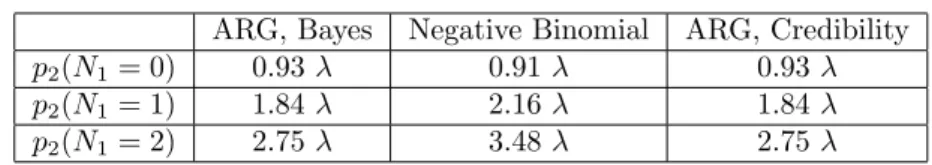
Case T = 1. Table 1 illustrates the posterior premium at period 2 according to the number of claims (which we limit to 2) in the first period. For ease of comparison, each premium is ex-pressed as a multiple ofλ. Nevertheless, the reader should keep in mind that these multiplicative coefficients depend also on the value ofλfor both models and both premium principle.
ARG, Bayes Negative Binomial ARG, Credibility
p2(N1= 0) 0.93λ 0.91λ 0.93λ
p2(N1= 1) 1.84λ 2.16λ 1.84λ
p2(N1= 2) 2.75λ 3.48λ 2.75λ
Table 1: Premium at the second period, according to the number of claims in the first period. The second column reports the Bayes premium obtained with the ARG model, the third column reports the Bayes premium obtained with the negative binomial model, and the last one reports the credibility premium of the ARG model.
14A copy of the programme is available from the author upon request.
15In a previous version of the paper available online, we also explain how to fit a dynamic frailty model with a more flexible autocorrelation function than the first order ARG process.
As expected, one or more claim results in an increase of the premium in each of the three columns. However, the size of the increase differs. For instance, if there is one (resp. two) claim at the first year, then the premium of the next year is given by (16) and is 1.84λ(resp. 2.75λ), that is an 84%(resp. 175%) increase. As a comparison, in the classical negative binomial model, the premium would have been: 0.0733+0.733+1.07λ= 2.16λ(0.0733+0.733+2.07λ= 3.48λ) that is more than 100
% (resp. 250 %) more expensive. This is due to the mean-reverting property of the dynamic frailty.
On the contrary, if there is no claim in the first year, the next year premium is 0.93λ, compared to 0.91λ in the negative binomial model. As a summary, our model provides a less severe post-claim malus, as well as a less generous non-claim bonus than that induced by the negative binomial model [a similar result is obtained for the linear credibility premium, see also Pinquet et al. (2001)].
Finally, let us remark that in Table 1, the credibility and Bayes premia are equal. This is expected, but is only true in the special case whereT = 1. Indeed, equation (16) shows that the conditional expectationE[U2|N1=n1]is a linear function of n1.
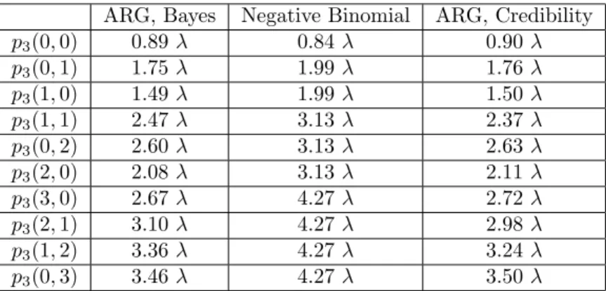
CaseT = 2. We now move to the posterior premium at period 3, according to the claim history of the two first periods. In particular, we will see that from now on, the credibility premium is generically biased with respect to the Bayes premium and the bias is path-dependent. For illustration purpose, in Table 2, we restrict ourselves to no more than 3 claims during the first two periods.
ARG, Bayes Negative Binomial ARG, Credibility
p3(0,0) 0.89λ 0.84λ 0.90λ p3(0,1) 1.75λ 1.99λ 1.76λ p3(1,0) 1.49λ 1.99λ 1.50λ p3(1,1) 2.47λ 3.13λ 2.37λ p3(0,2) 2.60λ 3.13λ 2.63λ p3(2,0) 2.08λ 3.13λ 2.11λ p3(3,0) 2.67λ 4.27λ 2.72λ p3(2,1) 3.10λ 4.27λ 2.98λ p3(1,2) 3.36λ 4.27λ 3.24λ p3(0,3) 3.46λ 4.27λ 3.50λ
Table 2: Premium for the third period, according to the number of claims in the first and second periods. For expository purpose we use the abbreviationp3(1,0) =p3(N1= 1, N2= 0), say.
We can see that the pricing error of the credibility approach with respect to the Bayes approach is large, so long as both N1 and N2 are non zero. In order to better understand
difference operators16:
∆xp3(x, y) :=p3(x+ 1, y)−p3(x, y), ∆yp3(x, y) :=p3(x, y+ 1)−p3(x, y),
∆2xxp3(x, y) := ∆x(∆xp3(x, y)) =p3(x+ 2, y) +p3(x, y)−2p3(x+ 1, y),
∆2xyp3(x, y) := ∆x(∆yp3(x, y)) =p3(x+ 1, y+ 1) +p3(x+ 1, y)−p3(x, y+ 1) +p3(x, y),
∆2yyp3(x, y) := ∆y(∆yp3(x, y)) =p3(x, y+ 2) +p3(x, y)−2p3(x, y+ 1), ∀x, y∈N.
In particular,∆yp3(x,0)is the bonus-malus factor of a non-claim second period. In order to save
space, the value of these finite differences are reported in Tables 1-5 of the online Appendix. From Tables 1 and 2 we can remark that, for both the negative binomial premium and the credibility premium, ∆xp3 and ∆yp3 are constant and therefore ∆2xxp3 = ∆2xyp3 = ∆2yyp3 = 0. This is
expected, since under these two pricing principles,p3 is a linear function of the two arguments
x, y.
Then we can remark that, for both the credibility and Bayes ARG model, we have always
∆xp3 < ∆yp3, in other words, the more recent claim has a larger impact on the posterior
premium. This is in contrast with the negative binomial model in which p3 depends only on
the total number of claims counts, and shows the interest of having a time-varying heterogeneity term.
Let us now discuss the second-order differences for the Bayes ARG model. We can see that
∆2
xxp3and∆2yyp3are generically different from zero, but are approximately zero whenx=y= 0,
whereas∆2
xyp3 is significantly positive, for allx+y≤1.For instance, we have:
∆2xyp3(0,0) = 0.12 = p3(1,1)−p3(0,0) −p3(1,0)−p3(0,0) −p3(0,1)−p3(0,0) ,
in other words the malus of having accidents at both the first and second period, that isp3(1,1)−
p3(0,0), is larger than the sum of the malus of having just one accident during the first and second
period, respectively. Equivalently, in terms of the bonus-malus factor, we have
p3(1,1)−p3(1,0) = 0.72λ > p3(0,1)−p3(0,0) = 0.60λ, (19)
which depends on the past claim history, and is increasing in the other variable, compared to the credibility premium formula which assumes it to be independent of x and y. This can be interpreted as the heteroscedasticity of the process (Ut) (and hence of process (Nt)). More precisely, the conditional expectationE[U1|N1] is larger if an individual has a claim at period
t = 1. Thus we also expect that when the information of N2 is incorporated, the updated
expectationE[U2|N1, N2], has a larger sensitivity inN2, ifN1 is equal to one.
This finding illustrates the bias, if the usual linear approximation in the credibility approach is to be used:
p3(x, y) =p3(0,0) + ∆xp3(0,0)x+ ∆yp3(0,0)y, ∀x, y∈N, (20)
Indeed when x, y are small but both are non zero, a convexity adjustment is needed in the previous expansion:
p3(x, y)≈p3(0,0) + ∆xp3(0,0)x+ ∆yp3(0,0)y+ ∆2xyp3(0,0)
xy
2 . (21)
Of course, the approximation (21) becomes less precise when at least one of x, yis large, since in that case the higher order terms ∆2
xxp3(0,0)x 2 2 and∆ 2 yyp3(0,0)y 2
2, or even third-order cross
terms∆3 xxyp3(0,0)x 2y 6 ,∆ 3 xyyp3(0,0)xy 2
6 become non negligible.
This analysis is also linked to a recent work of Le Courtois (2015), who proposes to improve the linear credibility formula by including quadratic termsx2,y2into the regression (20). Indeed,
(21) shows that at least in the ARG dynamic frailty model, the cross terms are more important than the squared ones. To some extent, this could be interpreted as the following. The squared terms are mainly intended to capture the non-Gaussian feature of themarginal distribution of eachNt, whereas the cross terms capture the non-linear, that is heteroscedastic feature of the
serial dependence. Finally, is∆2
xyp3(x, y)always positive for allx, y, and/or for all values ofλ1, λ2? The answer
is negative. In Figure 1 of the online Appendix, we plot the iso-contour of ∆2
xyp3(0,0) as a
function ofλ1andλ2, which we allow, momentarily, to be different17. We find that, for instance,
whenλ1 = 0.07 andλ2 = 0.2, that is when there is a sudden increase the value of the a priori
premium λin the second period, we have∆2
xyp3(0,0) =−0.03<0. However, when λ1, λ2 are
close to each other, the sign of∆2
xyp3(0,0)is always positive. Moreover, the value of∆2xyp3(x, y)
also depends on parameters of the ARG, that are(ρ, δ). In Figure 2 of the online Appendix, we plot the iso-contour of∆2xyp3(0,0)as a function ofρandδ, whenλ1, λ2are fixed to be 0.07. We
can see in particular that when δ is small, the value of∆2xyp3(0,0) is very large, and thus the
convexity adjustment term in equation (21) is very important.
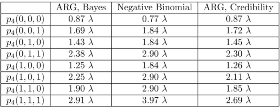
Case T = 3. Let us now move to the posterior premium for period T+ 1 = 4, based on the claim history of the three previous periods. Table 3 reports individuals with at most one claim
17In this exercise, we have kept the same values ofδandρ. Of course, the numerical results would be different when different values ofδandρare used.
during each period18.
ARG, Bayes Negative Binomial ARG, Credibility
p4(0,0,0) 0.87λ 0.77λ 0.87λ p4(0,0,1) 1.69λ 1.84λ 1.72λ p4(0,1,0) 1.43λ 1.84λ 1.45λ p4(0,1,1) 2.38λ 2.90λ 2.30λ p4(1,0,0) 1.25λ 1.84λ 1.26λ p4(1,0,1) 2.25λ 2.90λ 2.11λ p4(1,1,0) 1.90λ 2.90λ 1.85λ p4(1,1,1) 2.91λ 3.97λ 2.69λ
Table 3: Premium for the fourth period, according to the numbers of claims in the previous periods.
Similarly, for the Bayes ARG model, we can compute the first-order differences∆x, ∆y, ∆z
of the functionp4(x, y, z), as well as the second-order differences∆2xx,∆2yy,∆2zz,∆2xy,∆2yz,∆2zx.
Their values are reported in Tables 6-9 of the online Appendix. As expected, we obtain similar findings as in the caseT = 2, namely:
• ∆xp4<∆yp4<∆zp4, that is the importance of the observations in the premium function
decreases as the duration increases.
• At point(x, y, z) = (0,0,0), we have approximately∆2
xxp4= ∆2yyp4= ∆2zzp4= 0, whereas
the cross-differences∆2
xyp4,∆2yzp4,∆2zxp4are significantly positive. This explains why the
pricing bias of the credibility approach is generically larger whenever there are more than two claims during the previous periods. For instance, if there are one claim during each period, then the Bayes premium is 2.91λ, compared to the credibility premium 2.69λ.
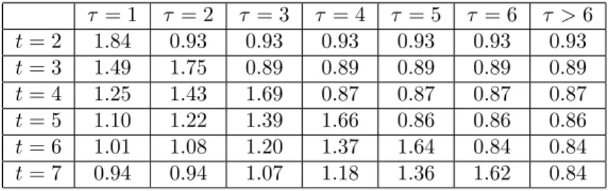
Evolution of the premium. Let us now illustrate the path-dependency of the Bayes pre-mium. In Table 4 we report the evolution of the Bayes premium an individual obtains at periods
t= 2,3, ...,7, before reporting its second claim. We denote byτthe timing of the first claim and distinguish seven cases: τ = 1,2, ...,6, or τ >6, corresponding the case of no claim in the first six years.
τ = 1 τ= 2 τ = 3 τ= 4 τ= 5 τ= 6 τ >6 t= 2 1.84 0.93 0.93 0.93 0.93 0.93 0.93 t= 3 1.49 1.75 0.89 0.89 0.89 0.89 0.89 t= 4 1.25 1.43 1.69 0.87 0.87 0.87 0.87 t= 5 1.10 1.22 1.39 1.66 0.86 0.86 0.86 t= 6 1.01 1.08 1.20 1.37 1.64 0.84 0.84 t= 7 0.94 0.94 1.07 1.18 1.36 1.62 0.84
Table 4: Evolution of the Bayes premium (divided byλ) for an individual before reporting the second claim.
For instance, column τ= 1reports the sequence of at periods2−7, if this individual has a first claim at period τ = 1, but does not report any claim in the subsequent periods. In other words, the six entries of this column are respectively: p2(1), p3(1,0), p4(1,0,0), p5(1,0,0,0),
p6(1,0,0,0,0), andp7(1,0,0,0,0,0), divided byλ. On the other hand, columnτ >6reports the
premium for an individual who has never reported claims, that is, the entries of that column are respectively: p2(0), p3(0,0),p4(0,0,0),p5(0,0,0,0), p6(0,0,0,0,0), andp7(0,0,0,0,0,0).
For each column, the sequence of premium is smaller than 1 and decreasing so long as there is no claim yet. In particular, in the last column, the premium of an individual who has never reported claims decreases and converges to a constant (0.84). This is the best “bonus premium” one can obtain. As a comparison, for the negative binomial model, the premium would have decreased towards zero if the individual never reports claim [see equation (2)]. However, this convergence rate is hyperbolic, thus much slower than in the dynamic frailty model. For instance, after six non-claim periods, the premium att = 7 obtained by the negative binomial model is 0.63. This is because our model assigns more weights to recent claims than the static model.
After the first claim, the premium jumps back to above 1. This new “malus premium” depends on the timing of the first claim and ranges from 1.84 for τ = 1 to 1.62 to τ = 6. The larger
τ, that is the larger the number of consecutive non-claim periods, the lower this first “malus premium”. In particular, for an individual who previously benefits the best premium 0.84, the malus premium is 1.62 (which corresponds to the entryt= 7, τ = 6.)
From the columnτ= 1, we observe that after the first claim att= 1, it takes the individual 4 consecutive periods of non-claim in order to get the premium1.01at the periodt= 6, which is approximately the initial, a priori premium. This waiting time is also decreasing in τ. For instance, columnτ= 2says that for an individual who has one non-claim period before the first claim, 4 consecutive non-claim periods after the first claim leads to a premium equal to 0.94.
5
A simple common factor bivariate extension
There is a growing interest in the literature to extend the standard univariate analysis to multiple count processes [see e.g. Frees (2003); Pinquet (1998); Englund et al. (2008, 2009); Abdallah et al. (2016); Berm´udez and Karlis (2015)]. For instance, a car insurance policy involves in general two types of coverage: the third-party liability and the (body and vehicle) casualty. This gives rise to a bivariate count process(N1,t, N2,t)t, which generically features positive correlation between the
two components, as well as serial correlation between different periods. The aim of this section is to briefly discuss a bivariate extension of our model. Let us assume thati), the unobservable factor(Ut)is, stationary ARG.ii), conditional on the entire trajectory of(Ut), pairs(N1,t, N2,t)t
are independent , and have the following stochastic representation:
N1,t=Z0,t+Z1,t, N2,t=Z0,t+Z2,t, (22)
where Z0,t, Z1,t, Z2,t are mutually independent, Poisson distributed conditionally on(Ut), with
parametersλ0,tUt, λ1,tUtandλ2,tUtrespectively, andλ0,t, λ1,t,λ2,t are observable up to a finite
number of parametersα.
This decomposition states that the occurrence of claims can be either due to third-party liability alone, or due to casualty alone, or due to both, although for each claim, this information is not necessarily available to the actuary19. This is usually called trivariate Poisson reduction
[see Gourieroux et al. (1984), Berm´udez and Karlis (2012)].
Thus the unobservable common factor process (Ut)introduces positive dependence between
N1,tandN2,t, as well as serial correlation. As a consequence, the past observations of both count
variables have prediction power.
Let us also remark thatN1,t(resp.N2,t) are conditionally Poisson distributed with parameter (λ0,t +λ1,t)Ut (resp. (λ0,t+λ2,t)Ut). Thus the marginal distributions of N1,t and N2,t are
conditionally Poisson (and marginally negative binomial), with a dynamic latent factor that is a autoregressive gamma process. In other words, in this bivariate model, each component count process is compatible with the univariate model described above. This compatibility is quite appealing, since usually the actuary has a portfolio of policyholders in which some choose two (or more) types of coverage, whereas others choose only one type. Thus a bivariate model that is not compatible with the marginal model is difficult to use on such a mixed portfolio.
6
Concluding remarks
This paper proposed a dynamic frailty model for count processes in Insurance, and extends the previous work by Pinquet et al. (2001); Bolanc´e et al. (2003); Brouhns et al. (2003). We showed how the estimation, premium updating as well as non-linear risk forecasting are greatly simplified within the same framework. In particular, in terms of pricing, we derived closed form formulas for theexact Bayes posterior premium. Using a numerical example on automobile insurance pricing, we illustrated how the posterior premium captures the non-linear, duration-dependent impact of past claim history on future ones, and evaluated the potential pricing bias, if a credibility approach were to be used instead. More precisely, the (linear) credibility approach mis-prices future risks by failing to account for a convexity adjustment, that is the surcharge of having accidents at several different periods, compared to the sum of marginal malus coefficients of individual accidents. As a by-product, our model suggests an improved quadratic credibility formula, when the modeller wants to use a specification of the underlying dynamic frailty that is different from ARG (and thus when the closed-form Bayes premium is not available):
pT+1(N1, N2, ..., NT) = T X t=1 atNt+ X 1≤t1<t2≤T bt1,t2Nt1Nt2.
This formula suggests several avenues for future research. First, is it possible to ensure the positivity of the regression coefficients? Second, when T is large, this formula involves the inversion of a high-dimensional (indeed T(T2+1)×T(T2+1)) matrix. Thus is it possible to impose some sparsity constraints on the matrix(bi,j), say,bi,j= 0so long as|i−j|is large enough?
Our key technical contribution is the introduction of the ARG dynamic frailty model. Indeed, besides the tractability it provides for estimation, pricing and forecasting in our specific applica-tion, this process has also the great advantage of belonging to the family of (discrete/continuous time) affine processes, which are very popular in Finance. Thus this framework is also quite ap-pealing for other insurance applications which involves financial risks, thanks to the compatibility it can provide. These situations have become quite standard nowadays due to the interconnect-edness between the two sectors. One typical example concerns the modelling of life-insurance lapses. In this case we can imagine an unobservable common risk factor which drives the process of monthly total number of lapses of an insurer. This avoids the use of ad hoc observable risk factors and thus provides more flexibility for risk analysis.
References
Abdallah, A., Boucher, J.-P., and Cossette, H. (2016). Sarmanov family of multivariate distri-butions for bivariate dynamic claim counts model. Insurance: Mathematics and Economics. Albrecht, P. (1985). An evolutionary credibility model for claim numbers. ASTIN Bulletin,
15(01):1–17.
Baione, F., Levantesi, S., and Menzietti, M. (2002). The development of an optimal bonus-malus system in a competitive market. Astin Bulletin, 32(01):159–170.
Berm´udez, L. and Karlis, D. (2012). A finite mixture of bivariate poisson regression mod-els with an application to insurance ratemaking. Computational Statistics & Data Analysis, 56(12):3988–3999.
Berm´udez, L. and Karlis, D. (2015). A posteriori ratemaking using bivariate poisson models. Scandinavian Actuarial Journal, pages 1–11.
Bolanc´e, C., Denuit, M., Guill´en, M., and Lambert, P. (2007). Greatest accuracy credibility with dynamic heterogeneity: the harvey-fernandes model. Belgian Actuarial Bulletin, 7(1):14–18. Bolanc´e, C., Guill´en, M., and Pinquet, J. (2003). Time-varying credibility for frequency risk
models: estimation and tests for autoregressive specifications on the random effects.Insurance: Mathematics and Economics, 33(2):273–282.
Brouhns, N., Guill´en, M., Denuit, M., and Pinquet, J. (2003). Bonus-malus scales in segmented tariffs with stochastic migration between segments.Journal of Risk and Insurance, 70(4):577– 599.
B¨uhlmann, H. (1967). Experience rating and credibility. Astin Bulletin, 4(03):199–207. B¨uhlmann, H. (1984). The general economic premium principle. Astin Bulletin, 14(01):13–21. Darolles, S., Gourieroux, C., and Jasiak, J. (2006). Structural laplace transform and compound
autoregressive models. Journal of Time Series Analysis, 27(4):477–503.
Davis, R. A., Dunsmuir, W. T., and Streett, S. B. (2003). Observation-driven models for poisson counts. Biometrika, 90(4):777–790.
Dionne, G. and Vanasse, C. (1989). A generalization of automobile insurance rating models: the negative binomial distribution with a regression component. Astin Bulletin, 19(2):199–212. Duffie, D., Filipovi´c, D., and Schachermayer, W. (2003). Affine Processes and Applications in
Englund, M., Guill´en, M., Gustafsson, J., Nielsen, L. H., and Nielsen, J. P. (2008). Multivariate latent risk: A credibility approach. Astin Bulletin, 38(01):137–146.
Englund, M., Gustafsson, J., Nielsen, J. P., and Thuring, F. (2009). Multidimensional credibility with time effects: an application to commercial business lines. Journal of Risk and Insurance, 76(2):443–453.
Frees, E. W. (2003). Multivariate credibility for aggregate loss models.North American Actuarial Journal, 7(1):13–37.
Frees, E. W. and Wang, P. (2005). Credibility using copulas. North American Actuarial Journal, 9(2):31–48.
Gerber, H. and Jones, D. (1975). Credibility formulas of the updating type. Transactions of the Society of Actuaries, 27:31–52.
Gourieroux, C. and Jasiak, J. (2004). Heterogeneous inar (1) model with application to car insurance. Insurance: Mathematics and Economics, 34(2):177–192.
Gouri´eroux, C. and Jasiak, J. (2006). Autoregressive Gamma Processes. Journal of Forecasting, 25(2):129–152.
Gourieroux, C. and Monfort, A. (1997). Simulation-based econometric methods. OUP Oxford. Gourieroux, C., Monfort, A., and Trognon, A. (1984). Pseudo maximum likelihood methods:
Applications to poisson models. Econometrica, pages 701–720.
Harvey, A. C. and Fernandes, C. (1989). Time series models for count or qualitative observations. Journal of Business & Economic Statistics, 7(4):407–417.
Heckman, J. J. (1987). The incidental parameters problem and the problem of initial conditions in estimating a discrete time-discrete data stochastic process and some monte carlo evidence. in Structural Analysis of Discrete Data, (ed) Charles F. Manski, Daniel Mcfadden.
Henderson, R. and Shimakura, S. (2003). A serially correlated gamma frailty model for longitu-dinal count data. Biometrika, 90(2):355–366.
Jewell, W. S. (1974). Credible means are exact bayesian for exponential families. Astin Bulletin, 8(01):77–90.
Le Courtois, O. (2015). q-credibility. Available at SSRN 2571195.
Lemaire, J. (1995). Bonus-malus systems in automobile insurance. Insurance Mathematics and Economics, 3(16):277.
Najafabadi, A. T. P. (2010). A new approach to the credibility formula.Insurance: Mathematics and Economics, 46(2):334–338.
Pinquet, J. (1998). Designing optimal bonus-malus systems from different types of claims. Astin Bulletin, 28(02):205–220.
Pinquet, J., Guill´en, M., and Bolanc´e, C. (2001). Allowance for the age of claims in bonus-malus systems. Astin Bulletin, 31(02):337–348.
Purcaru, O. and Denuit, M. (2003). Dependence in dynamic claim frequency credibility models. Astin Bulletin, 33(01):23–40.
Schrager, D. F. (2006). Affine stochastic mortality. Insurance: mathematics and economics, 38(1):81–97.
Sim, C.-H. (1990). First-order autoregressive models for gamma and exponential processes. Journal of Applied Probability, pages 325–332.
Sundt, B. (1988). Credibility estimators with geometric weights. Insurance: Mathematics and Economics, 7(2):113–122.
Tremblay, L. (1992). Using the poisson inverse gaussian in bonus-malus systems. Astin Bulletin, 22(01):97–106.
Varin, C., Reid, N., and Firth, D. (2011). An Overview of Composite Likelihood Methods. Statistica Sinica, 21(1):5–42.