Parameter Estimation of Smith Model
Max-Stable Process Spatial Extreme Value
(Case-Study: Extreme Rainfall Modelling in Ngawi Regency)
Siti Azizah1, Sutikno1, and Purhadi1
AbstractThe unpredictable extreme rainfall can affect flood. Prediction of extreme rainfall is needed to do, so that the efforts to preventing the flood can be effective. One of the methods that can predict the extreme rainfall is the Spatial Extreme Value (SEV) with the Max-Stable Process (MSP) approach. The important purpose of SEV is calculated of return level (the extreme value prediction). The calculation of return level depends on parameter estimation in that method. This research discusses about parameter estimation of the Spatial Extreme Value Max-Stable Process especially Smith model. Parameter estimation was performed using Maximum Composite Likelihood Estimation (MCLE) method and Maximum Pairwise Likelihood Estimation (MPLE) method. The result of estimation using this method is not closed form, it must be continued by using numerical iteration method. The iteration method used in this research is Broyden-Fletcher Goldfarb-Shanno (BFGS) Quasi Newton, which is faster than other methods to achieve convergence. The result of parameter estimation applied to the rainfall data of Ngawi Regency which is the Regency with the largest rice production in East Java Province (the province with the largest rice farm in Indonesia). Based on the results of data analysis obtained trend surface model µ̂(s) = 2,794+ 0,242 v(s);
𝝈̂(s) = 1,8196 + 0,1106 v(s); 𝝃̂(s) = 1,012 with goodness criterion model Takeuchi Information Criterion (TIC) 26237,62. Root Mean Square Error (RMSE) based on 20 testing data is 32,078 and Mean Absolute Percentage Error (MAPE) is 27,165%.
KeywordsBFGS Quasi Newton, Smith Model, Max-Stable Process, Maximum Pairwise Likelihood Estimation, Extreme rainfall, Return level.
I.INTRODUCTION1
he unpredictable extreme rainfall is cause of flood. Based on the reason, the extreme rainfall prediction needs to be done. One method to predict extreme rainfall value is Spatial Extreme Value (SEV). SEV can be approached by Max-Stable Process (MSP). The main goal of SEV is to acquire return level (prediction value of extreme happening). Return level can be acquired when a number of parameter estimators are known. Parameter estimation method which is mostly proposed by the previous researchers is Maximum Pairwise Likelihood Estimation (MPLE). This research estimates parameter toward Max-Stable Process (MSP), which involves one of its model, it is Smith Model. If the result of parameter estimation is not closed form, so that it must be continued by using numerical iteration method, in research, it will be used iteration method of Broyden-Fletcher Goldfarb-Shanno (BFGS) Quasi Newton.
II.METHOD
A. Extreme Value Theory
Extreme Value Theory (EVT) is a theory which studies about the probability of extreme happenings by focusing on the tail behavior of a distribution[1].
1Siti Azizah, Sutikno, and Purhadi are with Department of Statistics,
Institut Teknologi Sepuluh Nopember, Surabaya, 60111, Indonesia. E-mail: [email protected]; [email protected]; [email protected].
The tail behavior which declines slowly (the fat tail shape) indicates the existance of probability of extreme happenings. The fatter the tail of distribution is, the bigger the brobability of extreme value to appear. [2] and[3] explains that there are two methods of defining extreme value. They are BM and Peak Over Threshold (POT).
Extreme Value Theory involves a distribution for generalizing extreme data into distribution of GEV[4].
X~GEV(µ, α, ξ) has the form of Probability Density Function(PDF) f(x; µ, σ, ξ) = { 1 σ[1 + 𝜉 (𝑥−µ) 𝜎 ] −1 ξ−1 exp (– [1 + 𝜉(𝑥−µ) 𝜎 ] −1/ξ ) , 𝜉 ≠ 0 1 σexp (− 𝑥−µ σ ) exp (−exp [− (𝑥−µ) 𝜎 ]) , 𝜉 = 0 (1)
X is variable of observation, µ is parameter of location, σ is parameter of scale, σ > 0, and ξ is parameter of shape. Parameter ξ indicates tail behavior of GEV. Based on parameter ξ, GEV distribution follows Gumbel distribution when ξ = 0, follows Frechet distribution when ξ > 0, and follows Weibull distribution when ξ < 0.
B. Spatial Extreme Value
There are many data of observation connected with natural happening, they are the data from a happening in a small area in the larger area. Based on the data, it is possible that there is dependency between one spot to another spot in one area of happening. The nearer the distance (h) between locations, it is possible that there is dependency which is more stronger. The distance between locations (s) to-j and to-k can be counted by using distance measurement with equation of
hj,k =|| sj - sk || (2) u is longitude of location (s), v is latitude of location (s).
Z = (1 + 𝜉𝑋−µ
𝜎 )+ 1/𝜉
(3)
C. Max-Stable Process
Max-Stable Process (MSP) is stocastical process, the enlargement of distribution of multivariate extreme value to the infinity dimension. {𝑍(𝑠)}𝑠𝜖ℝ𝑑is said max-stableif a
constantan (s) > 0 and bn(s) ϵ R, so Z(s) = lim 𝑛→+∞ max𝑖=1𝑛 {𝑥𝑖(𝑠)}−𝑏𝑛(𝑠) 𝑎𝑛(𝑠) , n→ ∞, 𝑠 ∈ ℝ 𝑑 (4)
xi(s) distributes identical independent random[5].
Z(s) is said max-stable if and only if follows distribution of GEV which constitutes distribution for extreme happening data. Frechet distribution has the fattest shape of tail compared with Gumbel and Weibull distribution. So, if
an (s) = n, bn(s) = 0, Z(s) = 0, Z(s) can be generalized into Frechet unit. F(z) = exp(−1 𝑍 ), z> 0 (5) Z is form of transformation of X, Z = (1 + 𝜉𝑋−µ 𝜎 )+ 1/𝜉 (6) D. Block Maxima
Block Maxima(BM) is extreme value identification method based on the formation of period blocks. The data of observation are devided into certain blocks. Based on the formed blocks, it is choosen the maximum value of observation of each block. The choosen maximum value of each block belongs to extreme sample. Extreme value which is taken using BM method follows GEV distribution. E. Model Smith CDF Model of Smithis F(zj,zk)=exp(− 1 𝑍𝑗𝛷 ( 𝑎(ℎ) 2 + 1 𝑎(ℎ)𝑙𝑜𝑔 [ 𝑍𝑘 𝑍𝑗]) − 1 𝑧𝑘𝛷 ( 𝑎(ℎ) 2 + 1 𝑎(ℎ)𝑙𝑜𝑔 [ 𝑍𝑗 𝑍𝑘])) (7)
zj is variable Z location to-j, zk is variable Z location to-k,Φ is CDF bivariat normal standard, a(hj,k) is √𝒉𝒋,𝒌𝑇𝜮𝒋,𝒌−1𝒉𝒋,𝒌, and Σj,k is matrix covarian of location
variable to-j and to-k[6].
F. Extremal Coefficient
Extremal coefficient constitutes coeficient used to see dependency level between one variable with another variable. Extremal coeficient of Smith Model MSP has the range of value 1 ≤ 𝛳(𝒉𝒋,𝒌) ≤2. The more approaching the
value of ϴ(hj,k) to 1 indicates the more dependent between
the two variables. Extremal coeficient of Smith MSP Model is [7]
ϴ(hj,k) = 2Φ(
√𝒉𝒋,𝒌𝑇𝚺𝒋,𝒌−1𝒉𝒋,𝒌
2 ) (8)
G. Return Level
Return level is maximum value which can be achieved in certain period. Return level value constitutes the extreme value of prediction. Return levelfora location (s) is zp(s) = µ̂(s) – 𝜎 ̂(𝑠) 𝜉̂(𝑠)(1 − [− ln (1 − 1 T ) ] −ξ̂(s) ) (9)
T is the number of blocks in one interval of the predicted period. The achieved probability of zp(s) is
p = P ( Z > zp ) = 1
𝑇 (10)
H. Takeuchi Information Criterion
The result of parameter estimationof Smithproduces the value of β which is used to form Trend Surface Model. Trend Surface Model is linear model which combines coordinate variable of one spot or location, it constitutes lon (longitude) variable and lat (latitude) variable, parameter of β. Moreover the best Trend Surface Model of a number of combination is used for estimating return level. Determination of the best Trend Surface Model is done by counting the value of Takeuchi Information Criterion (TIC). Model with the least TIC value constitutes the best model [8].
TIC = -2 lp(𝜷̂) + 2 tr [J(𝜷̂)H(𝜷̂)-1] (11) With :
lp(𝜷̂) = function of lnpairwise likelihood
∑ ∑ ∑𝑚 𝑙𝑛 (𝑓(𝑧𝑗𝑖, 𝑧𝑘𝑖; 𝜷̂)) 𝑘=𝑗+1 m−1 j=1 n i=1 H(𝜷̂) = -∂2𝑙𝑝(𝜷̂) ∂𝜷̂ ∂𝜷̂T J(𝜷̂) = ∑ {(∂ ∑ ∑ 𝑙𝑛(𝑓(𝑧𝑗𝑖,𝑧𝑘𝑖;𝜷̂)) 𝑚 𝑘=𝑗+1 m−1 j=1 𝜷̂ ) 𝑛 𝑖=1 x (∂ ∑ ∑𝑚 𝑙𝑛 (𝑓(𝑧𝑗𝑖, 𝑧𝑘𝑖; 𝜷̂)) 𝑘=𝑗+1 m−1 j=1 𝜷̂ ) T}
I. Maximum Pairwise Likelihood Estimation
Maximum Pairwise Likelihood Estimation(MPLE) is parameter estimation method using the function of density pairwise or in pair of two variables. MPLE method replaces the function (L(β)) in Maximum Likelihood Estimation(MLE) with the function of pairwise likelihood
Lp(β).
Lp(β) = ∏𝑖=1𝑛 ∏𝑗=1𝑚−1∏𝑚𝑘=𝑗+1𝑓(𝑥𝑗𝑖, 𝑥𝑘𝑖; 𝜷) (12)
Estimator of parameter of ϴ (ϴ in this research is parameter of µ, σ, and ξ) is acquired from counting the first deferential of the function and equalize it with zero.
𝜕 𝑙𝑛 𝐿(𝜭)
𝜕𝜭 = 0 (13)
if and only if
𝜕𝐿(𝜭)
𝜕𝜭 = 0 (14)
So, it can be acquired the maximum estimator of ϴ more easily by the counting in ln L(ϴ) [9].
( ) ( ) arg min k k k k f S
( )
( ) k k k S H g
( ) ( 1) ( ) (23) k k k J. Anderson DarlingTestAnderson Darling (AD) Test is a test used to find out whether a date follows certain distribution. GEV distribution testing toward two extremes can be done by using Anderson Darling test with the following procedure [10] :
1) Hypothesis formulation :
H0 : F(X) = F*(X) (Data follows F*(X) theoretical distribution)
H1 : F(X) ≠ F*(X) (Data doesn’t follow F*(X) theoretical distribution)
In the case of rainfall, theoretical distribution used is GEV distribution 2) Statistics test 𝐴𝐷 = −𝑛 −1 𝑛∑ (2𝑖 − 1) 𝑛 𝑖=1 (𝑙𝑛𝐹 ∗ (𝑥𝑖) + 𝑙𝑛(1 − 𝐹 ∗ (𝑥𝑛+1−𝑖))) (15) F(X) is CDF of sample data F*(X) is theoretical CDF 3) Criterion of tes
Ignore H0 if AD value > critical value or p-value< α.
K. Rainfall
Rainfall is the altitude of rain water compiled in a rain meter on the flat place, not to absorb, not to permiate, and not to flow. Extreme raifall is rainfall which has intensity of >100 millimeter per day. Rainfall with intensity of > 50 millimeter per day constitutes heavy rainfall. Based on the classification of monthly average rainfall distribution pattern in all Indonesia areaconsists of 342 Zone of Season patterns, and 65 Non Zone of Season. Zone of Season is an area which average rain pattern has clear limit climatologically between dry season period and rainy season period. One regency or city may consist of some Zone of Season. Non Zone of Season is an area which doesn’t have the clear limit climatologically between rainy season period and dry season[11].
III.RESULT AND ANALYSIS
A. Smith Model Parameter Estimation Using MPLE
( ) 1 log 2 ( ) k j Z Z h w a h a ( ) 1 log 2 ( ) j k Z v Z a h a h 2 2 2 2 2 2 2 2 ( ) ( ) ( ) ( ) ( ) ( ) exp ( , ) j k j k j j j k k k j k j k j k w v Z Z w w v Z Z Z Z v v w Z Z Z Z v w w a h a h a h a h a h a v Z Z h Z Z f X X (16)
1 1 1 1 2 2 2 2 2 , 1 1 1 1 2 2 2( ) z
,
exp
( ) z
( ) z
( ) z
( )
( )
n m m i j k j ji ki ji ki ji ji ji ki ki ki ji ki ji ki p µ n m m i j k jw
v
z
z
w
w
v
z
z
v
v
w
z
z
v w
w v
L
a h
a h
a h
z
a h
a
h
z
a h z z
β β β
(17)The next step is make ln likelihood (Appendix 1). With
µ(s)= dT
µ σ(s)= dT ξ(s)= u(s) and v(s) is longitude and latitude of location, ln likelihood function becomes new form (Appendix 2).
The next step is derivate this equation to every parameter (βµ, βσ, and βξ). Estimation using MPLE gives a result in the form of equation which is very complex and not closed form. The estimation of parameter must be continued by numerical iteration in this research is BFGS Quasi Newton.
B. Quasi Newton BFGS Iteration Algorithm
1) Determining
0 which can be filled with matrix px1 with all its member is zero. p is the number of parameter. 2) Determining (19) 3) Determining matrixH(k1)
( ) ( ) ( ) ( ) ( ) ( 1) ( ) ( ) ( ) ( ) ( ) ( ) ( ) ( ) ( ) ( ) ( ) ( ) ( ) 1 (20) T k k k k k T k k T k T k k k T k k k T k k k T T k k g H g H H g g H g H g g H(0) =I (matrix identity in size of p
( )
( 1)
( )
(21) k k k g g g 4) Determining matrix
kg which elements containing
the first derivation of
kDetermining (22)
5) Doing numerical iteration by using equation k 1 k k k S (23) 6) Calculating (24) 7) Back to the process number 2 up to the process number
7.
8) Back to the process number 2 up to the process number 7.
Iteration is started from k = 1 and finished if with e is very small value.
( 1) ( )
C. Application to Real Data 1) The sample data
The sample data in this case study is an extreme values of rainfall data at 9 rainfall post (stations) in Ngawi. The samples were carried out using the method of Block Maxima (BM)
2) Determination of Data Sample.
Selection of extreme values is done by forming three-month blocks. Block formed is December-January-February (DJF), March-April-May (MAM), Jun-Jul-of August (JJA), and September-October-November (SON). During the 26 years of the sample period (1990-2015) was formed 103 blocks. Taken the maximum value of each block. 103 fetched the data, here's a sample of extreme events.
3) Distribution Testing.
Data can be approximated by Max-Stable Process (MSP) if the data follows the Generalized Extreme Value (GEV) distribution. TABLE 1. DISTRIBUTION TESTING Rainfall Stations Statistics Test Conclusion AD Value P-Value
Kendal 0,666 0,946 Following GEV
Legundi 0,913 0,994 Following GEV
Gentong 0,495 0,851 Following GEV
Paron 0,225 0,239 Following GEV
Gemarang 0,730 0,968 Following GEV
Kricak 0,504 0,865 Following GEV
Widodaren 1,642 0,999 Following GEV
Kedungharjo 0,691 0,971 Following GEV
Guyung 0,535 0,879 Following GEV
4) Measurement Dependencies
Here is an illustration of the results of the calculation coefficient extremal between sites of rainfall stations. The dependency between sites is positive slowly.
Figure 1.Graph Extremal Coefficient
5) The arrangement of the best Trend Surface Model
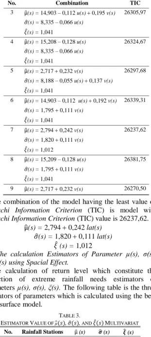
TABLE 2.
COMBINATION OF TREND SURFACE MODEL
No. Combination TIC
1 µ̂(s) = 14,903– 0,112 u(s) + 0,195 v(s) 26329,20 𝜎̂(s) = 8,195 – 0,059 u(s) 0,089 v(s) 𝜉̂(s) = 2 µ̂(s) = 15,208– 0,128 u(s) 26358,00 𝜎̂(s) = 8,195– 0,059 u(s)0,089 v(s) 𝜉̂(s) = 1,041 TABLE 2.(CONTINUED)
No. Combination TIC
3 µ̂(s) = 14,903 – 0,112 u(s) 0,195 v(s) 26305,97 𝜎̂(s) = 8,335– 0,066 u(s) 𝜉̂(s) = 1,041 4 µ̂(s) = 15,208– 0,128 u(s) 26324,67 𝜎̂(s) = 8,335– 0,066 u(s) 𝜉̂(s) = 1,041 5 µ̂(s) = 2,717 0,232 v(s) 26297,68 𝜎̂(s) = 8,188– 0,055 u(s)0,137 v(s) 𝜉̂(s) = 1,041 6 µ̂(s) = 14,903–0,112 u(s) 0,192 v(s) 26339,31 𝜎̂(s) = 1,7950,111 v(s) 𝜉̂(s) = 1,041 7 µ̂(s) = 2,794 0,242 v(s) 26237,62 𝜎̂(s) = 1,8200,111 v(s) 𝜉̂(s) = 1,012 8 µ̂(s) = 15,209– 0,128 u(s) 26381,75 𝜎̂(s) = 1,7950,111 v(s) 𝜉̂(s) = 1,041 9 µ̂(s) = 2,717 0,232 v(s) 26270,50 The combination of the model having the least value of
Takeuchi Information Criterion (TIC) is model with
Takeuchi Information Criterion (TIC) value is 26237,62.
µ̂(s) = 2,794 0,242 lat(s) 𝜎̂(s) = 1,820 0,111 lat(s)
𝜉̂ (s) = 1,012
6) The calculation Estimators of Parameter µ(s), σ(s), ξ(s) using Spacial Effect.
The calculation of return level which constitute the prediction of extreme rainfall needs estimators of parameters µ(s), σ(s), ξ(s). The following table is the three estimators of parameters which is calculated using the best trend surfacemodel.
TABLE 3.
ESTIMATOR VALUE OF µ̂(𝑠),𝜎̂(𝑠),AND 𝜉̂(𝑠)MULTIVARIAT
No. Rainfall Stations µ̂ (s) 𝝈̂ (s) 𝝃̂ (s) 1 Kendal 0,965 0,983 1,012 2 Legundi 0,988 0,994 1,012 3 Gentong 0,979 0,990 1,012 4 Paron 0,994 0,997 1,012 5 Gemarang 1,004 1,001 1,012 6 Kricak 1,005 1,002 1,012 7 Widodaren 1,007 1,003 1,012 8 Kedungharjo 1,007 1,003 1,012 9 Guyung 1,007 1,003 1,012 7) Validation Model
The calculation of validation is done by using Root Mean Square Error (RMSE) value which is acquired 32,078. The Mean Absolute Percent Error (MAPE) value which is acqiured 27,165%
IV.CONCLUSION
The parameter estimation Smith Model of Max-Stable Process (MSP) can be done by using Maximum Pairwise 0.0 0.1 0.2 0.3 0.4 1 .0 1 .2 1 .4 1 .6 1 .8 2 .0 h h
Likelihood Estimation (MPLE) method. This parameter estimation produces the equation which is not closed form so that it must be continued by using numerical iteration. One of them is by using Broyden-Fletcher Goldfarb-Shanno(BFGS) Quasi Newton method which has the over plus, it is faster to reach convergence. The trend surface model for Extreme rainfall data in Ngawi Regency is
µ̂(s) = 2,794 0,242 lat(s) 𝜎̂(s) = 1,820 0,111 lat(s)
𝜉̂ (s) = 1,012
Its TIC value is 26237,62, Root Mean Square Error
(RMSE) value is 32,078 , and Mean Absolute Percentage Error (MAPE) value is 27,165%.
REFERENCES
[1] A. C. Davison, S. A. Padoan, and M. Ribatet, “Statistical Modeling of Spatial Extremes 1,” vol. 27, no. 2, pp. 161–186, 2012.
[2] M. Gilli and E. këllezi, “An Application of Extreme Value Theory for Measuring Financial Risk,” Comput. Econ., vol. 27, no. 2, pp. 207–228, 2006.
[3] S. A. Padoan, M. Ribatet, and S. Sisson, “Likelihood-based inference for max-stable processes,” J. Am. Stat. Assoc., vol. 105, no. 489, pp. 263–277, 2010.
[4] A. F. Jenkinson, “The frequency distribution of the annual maximum (or minimum) values of meteorological elements,” Q. J. R. Meteorol. Soc., vol. 81, no. 348, pp. 158–171, 1955.
[5] J. Blanchet and A. C. Davison, “Spatial modeling of extreme snow depth,” Ann. Appl. Stat., vol. 5, no. 3, pp. 1699–1725, 2011. [6] R. L. Smith, “Max-Stable Processes and Spatial Extreme,” 1990. [7] M. Schlather and J. A. Tawn, “A dependence measure for
multivariate and spatial extreme values: Properties and inference,”
Biometrika, vol. 90, no. 1, pp. 139–156, 2003.
[8] K. Takeuchi, “Distribution of informational statistics and a criterion of model fitting,” Math. Sci., vol. 153, pp. 12–18, 1976.
[9] R. M. Kozelka, Elements of Statistical Inference. Addison-Wesley Pub. Co., 1961.
[10] S. Engmann, “Quantitative Methods Inquires Comparing Distributions : The Two-Sample Anderson-Darling Test as An Alternative to The Kolmogorov-Smirnoff Test,” J. Appl. Quant. Methods, vol. 6, no. 3, pp. 1–17, 2011.
[11] BMKG, “Daftar Istilah Klimatologi,” 2014. [Online]. Available: http://balai3.denpasar.bmkg.go.id/daftar-istilah-musim. [Accessed: 25-Feb-2016].