A Comparison of Two MCMC Algorithms for Estimating the 2PL IRT Models

Dissertations Theses and Dissertations

8-1-2017

A Comparison of Two MCMC Algorithms for

Estimating the 2PL IRT Models

Meng-I Chang

Southern Illinois University Carbondale, [email protected]

Follow this and additional works at:http://opensiuc.lib.siu.edu/dissertations

This Open Access Dissertation is brought to you for free and open access by the Theses and Dissertations at OpenSIUC. It has been accepted for inclusion in Dissertations by an authorized administrator of OpenSIUC. For more information, please [email protected].

Recommended Citation

Chang, Meng-I, "A Comparison of Two MCMC Algorithms for Estimating the 2PL IRT Models" (2017).Dissertations. 1446. http://opensiuc.lib.siu.edu/dissertations/1446

IRT MODELS

by Meng-I Chang

B.S., Chung Yuan Christian University, Taiwan, 2001 M.A., Southern Illinois University Carbondale, 2008

A Dissertation

Submitted in Partial Fulfillment of the Requirements for the Degree of Doctor of Philosophy

Department of Counseling, Quantitative Methods, and Special Education in the Graduate School

Southern Illinois University Carbondale August 2017

A COMPARISON OF TWO MCMC ALGORITHMS FOR ESTIMATING THE 2PL IRT MODELS

by Meng-I Chang

A Dissertation Submitted in Partial Fulfillment of the Requirements

for the Degree of Doctor of Philosophy

in the field of Counseling, Quantitative Methods, and Special Education

Approved by:

Yanyan Sheng, Ph.D., Chair Todd Headrick, Ph.D. Rhonda Kowalchuk, Ph.D.

David Olive, Ph.D. John Reeve, Ph.D.

Graduate School

Southern Illinois University Carbondale June 2, 2017

MENG-I CHANG, for the Doctor of Philosophy degree in Counseling, Quantitative Methods, and Special Education, presented on June 2, 2017 at Southern Illinois University Carbondale. TITLE: A COMPARISON OF TWO MCMC ALGORITHMS FOR ESTIMATING THE 2PL IRT MODELS

MAJOR PROFESSOR: Dr. Yanyan Sheng

The fully Bayesian estimation via the use of Markov chain Monte Carlo (MCMC) techniques has become popular for estimating item response theory (IRT) models. The current development of MCMC includes two major algorithms: Gibbs sampling and the No-U-Turn sampler (NUTS). While the former has been used with fitting various IRT models, the latter is relatively new, calling for the research to compare it with other algorithms. The purpose of the present study is to evaluate the performances of these two emerging MCMC algorithms in estimating two two-parameter logistic (2PL) IRT models, namely, the 2PL unidimensional model and the 2PL multi-unidimensional model under various test situations. Through investigating the accuracy and bias in estimating the model parameters given different test lengths, sample sizes, prior specifications, and/or correlations for these models, the key

motivation is to provide researchers and practitioners with general guidelines when it comes to estimating a UIRT model and a multi-unidimensional IRT model. The results from the present study suggest that NUTS is equally effective as Gibbs sampling at parameter estimation under most conditions for the 2PL IRT models. Findings also shed light on the use of the two MCMC algorithms with more complex IRT models.

There are many individuals whom I would like to thank for helping me in completion of this dissertation. First, I would like to express my sincere gratitude and thanks to my advisor, Dr. Yanyan Sheng. Without her encouragement, guidance, and patience throughout my entire doctoral study, this dissertation would never have taken shape. She always made time for me no matter how busy she was when I needed her help. I really appreciate her for unsparingly

imparting her knowledge and expertise in this dissertation. I also would like to thank my other committee members, Dr. David Olive, Dr. John Reeve, Dr. Rhonda Kowalchuk, and Dr. Todd Headrick for their insightful comments and valuable suggestions, which inspired me to widen my dissertation from various perspectives.

My appreciation would also goes to my colleagues in the department, present and past, who provided a friendly and supportive environment to work and learn. Also, I would like to thank my friend, Tzu-Chun Kuo who has provided tremendous encouragement and help during my doctoral life.

Last but not the least, I would like to express my gratitude to my parents, brothers, and sister-in-law for their unconditional love and support even though they are 8000 miles away. Thank them for believing in me and helping me achieve my dreams.

CHAPTER PAGE

ABSTRACT....……….……….……….. i

ACKNOWLEDGMENTS ……….………....……… ii

LIST OF TABLES………….……… vi

LIST OF FIGURES ……….………...………...ix

CHAPTERS CHAPTER 1 – INTRODUCTION………...……….………..…1

1.1Statement of the Problem……….………..…7

1.2Purpose of the Study………..8

1.3Research Questions………....8

1.4Definition of Terms………...….8

1.5Significance of the Research………...………...…..11

1.6Delimitation of the Study………...………..…11

1.7Overview of Subsequent Chapters………...………..…..12

CHAPTER 2 – LITERATURE REVIEW….………..……….………..…...13

2.1 Item Response Theory…………..………..…….13

2.1.1 IRT Major Assumptions.…….………..………..…. 14

2.1.2 Unidimensional IRT (UIRT) Models…….………..………..…...15

2.1.3 Multidimensional IRT (MIRT) Models……….…..………..18

2.1.4 Multi-unidimensional IRT Model ………...………..19

2.2 Parameter Estimation of UIRT Model...20

2.2.1 Joint Maximum Likelihood (JML)……….21

2.2.3 Bayesian Estimation………...23

2.3 Parameter Estimation of MIRT Models………...26

2.4 MCMC Algorithms………....27

2.4.1 Random Walk MCMC Algorithms………....29

2.4.2 Other MCMC Algorithms………..31

2.4.3 Implementation of MCMC……….32

2.5 Prior Research Using Fully Bayesian with IRT Models………....34

2.5.1 UIRT Models Using Random Walk MCMC Algorithms………..34

2.5.2 MIRT Models Using Random Walk MCMC Algorithms……….35

2.5.3 IRT Models Using NUTS………...37

CHAPTER 3 – METHODOLOGY….………..…...……….39

3.1 Research Questions………....39

3.2 Simulation Study 1………... .39

3.2.1 Model……….40

3.2.2 Simulation Procedure……….40

3.2.3 Measures of Estimation Accuracy………...42

3.3 Simulation Study 2……….45

3.3.1 Model……….45

3.3.2 Simulation Procedure……….45

3.3.3 Measures of Estimation Accuracy……….47

CHAPTER 4 – RESULTS……….48

4.1 Results for the 2PL UIRT Model…… ……….………....48

4.1.2 Person Ability Parameter Recovery……….………...……..55

4.1.3 Analysis of Variance (ANOVA) Results for the 2PL UIRT Model……….57

4.2 Results for the 2PL Multi-unidimensional IRT Model….………59

4.2.1 Item Parameter Recovery………..………59

4.2.2 Person Ability Parameter Recovery…..………...….68

4.2.3 ANOVA Results for the 2PL Multi-unidimensional IRT Model………..71

CHAPTER 5 − DISCUSSION AND CONCLUSION……….………....77

5.1 Comparison of Gibbs Sampling and NUTS for the 2PL IRT Models….………..77

5.1.1 Model Parameters Recovery for the 2PL UIRT Model………..……….77

5.1.2 Model Parameters Recovery for the 2PL Multi-unidimensional IRT Model..…80

5.1.3 Computational Speed of Gibbs Sampling and NUTS………..…………82

5.2 Limitations and Directions for Future Studies………..83

REFERENCES……….………..………...86 APPENDICES Appendix A ………...102 Appendix B ………...107 VITA………...………..………...115 v

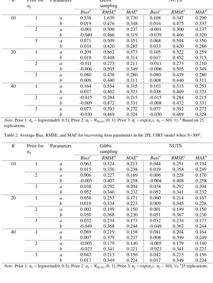
Table 1 Average Bias, RMSE, and MAE for recovering item parameters in the 2PL UIRT

model when N=100. ……….….53

Table 2 Average Bias, RMSE, and MAE for recovering item parameters in the 2PL UIRT

model when N=300. …..………..……….…….53

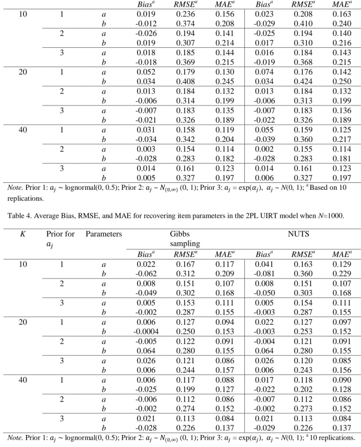
Table 3 Average Bias, RMSE, and MAE for recovering item parameters in the 2PL UIRT

model when N=500. .……….………..54

Table 4 Average Bias, RMSE, and MAE for recovering item parameters in the 2PL UIRT

model when N=1000…………...… … ………....54

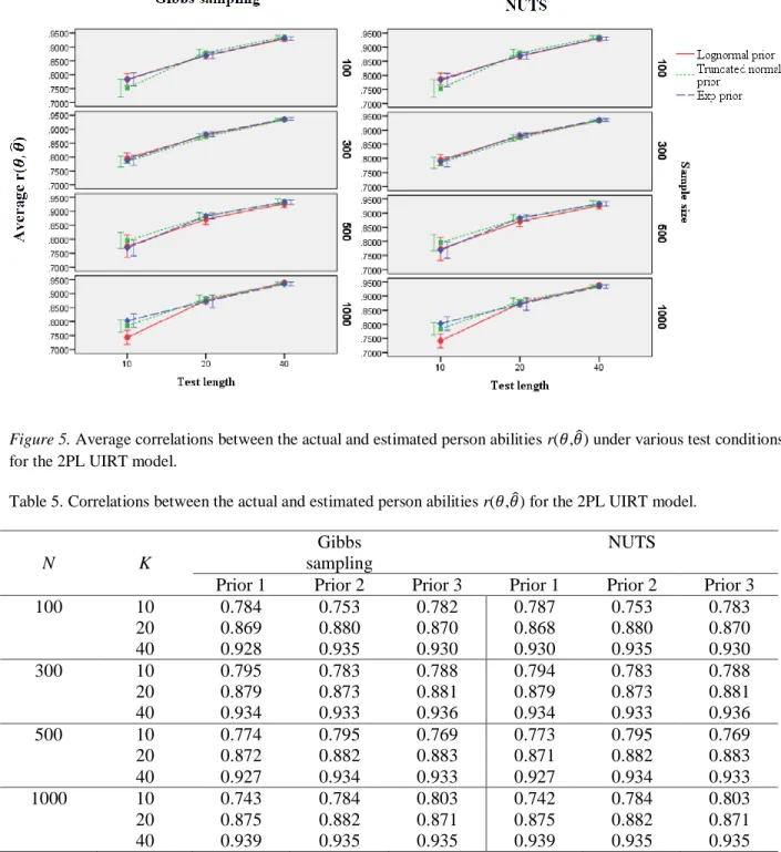
Table 5 Correlations between the actual and estimated person abilities r(𝜃,𝜃̂) for the 2PL

UIRT model…………...……….56

Table 6 ANOVA effect sizes (𝜔̂2_{) for logRMSE and logMAE in estimating the discrimination}

(a), difficulty (b) parameters, and 𝑟(𝜃, 𝜃̂) in the 2PL UIRT model…....…...………..58

Table 7 Average Bias, RMSE, and MAE for recovering item parameters in the 2PL multi-

unidimensional IRT model when N=100.……….………..……….. 64

Table 8 Average Bias, RMSE, and MAE for recovering item parameters in the 2PL multi-

unidimensional IRT model when N=300. ………...……….65

Table 9 Average Bias, RMSE, and MAE for recovering item parameters in the 2PL multi-

unidimensional IRT model when N=500. ………...…………...…………..66

Table 10 Average Bias, RMSE, and MAE for recovering item parameters in the 2PL multi-

unidimensional IRT model when N=1000………... ………67

Table 11 Correlations between the actual and estimated person abilities r(𝜃1,𝜃̂1) and

r(𝜃₂,𝜃̂₂) for the 2PL multi-unidimensional IRT model. ………..…...………. 71

Table 12 ANOVA effect sizes (𝜔̂2_{) for logRMSE in estimating the discrimination (𝑎}

1,𝑎2),

difficulty (𝑏_1,𝑏₂) parameters, r(𝜃₁,𝜃̂₁), and r(𝜃₂,𝜃̂₂) in the 2PL multi-unidimensional

IRT model………...………..………..75 Table A1 The true and estimated values of the item parameters in the 2PL UIRT model

using MML, Gibbs sampling, and NUTS when N=10. …………...……….104

Table A2 The true and estimated values of the item parameters in the 2PL UIRT model

using MML, Gibbs sampling, and NUTS when N=50. ………....………...……….105

Table A4 The true and estimated values of the item parameters in the 2PL UIRT model using

MML, Gibbs sampling, and NUTS when N=1000 and extremely easy items……..106

Table A5 The true and estimated values of the item parameters in the 2PL UIRT model using

MML, Gibbs sampling, and NUTS when N=1000 and extremely difficult items…106

Table B1 ANOVA effect sizes (𝜔̂2_{) for logRMSE in estimating the discrimination (a)}

parameters in the 2PL UIRT model. …………....………107

Table B2 ANOVA effect sizes (𝜔̂2) for logMAE in estimating the discrimination (a)

parameters in the 2PL UIRT model. …………...………..………...107

Table B3 ANOVA effect sizes (𝜔̂2) for logRMSE in estimating the difficulty (b)

parameters in the 2PL UIRT model.………..………...108

Table B4 ANOVA effect sizes (𝜔̂2_{) for logMAE in estimating the difficulty (b)}

parameters in the 2PL UIRT model. …………..………..108

Table B5 ANOVA effect sizes (𝜔̂2) for correlations between 𝜃 and 𝜃̂ in the 2PL UIRT

Model...………..109

Table B6 ANOVA effect sizes (𝜔̂2) for logRMSE in estimating the discrimination (𝑎₁)

parameters in the 2PL multi-unidimensional IRT model. …………..……….109

Table B7 ANOVA effect sizes (𝜔̂2) for logMAE in estimating the discrimination (𝑎1)

parameters in the 2PL multi-unidimensional IRT model. …...………...…….……110

Table B8 ANOVA effect sizes (𝜔̂2_{) for logRMSE in estimating the discrimination (𝑎}

2)

parameters in the 2PL multi-unidimensional IRT model. …………..……….……110

Table B9 ANOVA effect sizes (𝜔̂2) for logMAE in estimating the discrimination (𝑎₂)

parameters in the 2PL multi-unidimensional IRT model. …..…………..…..…….111

Table B10 ANOVA effect sizes (𝜔̂2) for logRMSE in estimating the difficulty (𝑏1)

parameters in the 2PL multi-unidimensional IRT model. ...………...……111

Table B11 ANOVA effect sizes (𝜔̂2) for logMAE in estimating the difficulty (𝑏1)

parameters in the 2PL multi-unidimensional IRT model.……...………..……….112

Table B12 ANOVA effect sizes (𝜔̂2_{) for logRMSE in estimating the difficulty (𝑏}

2)

parameters in the 2PL multi-unidimensional IRT model. ……….………112

Table B13 ANOVA effect sizes (𝜔̂2) for logMAE in estimating the difficulty (𝑏2)

Table B14 ANOVA effect sizes (𝜔̂2) for correlations between 𝜃1 and 𝜃̂1 in the 2PL

multi-unidimensional IRT model. ……….…………..……….113

Table B15 ANOVA effect sizes (𝜔̂2) for correlations between 𝜃2 and 𝜃̂2 in the 2PL

multi-unidimensional IRT model. ……….114

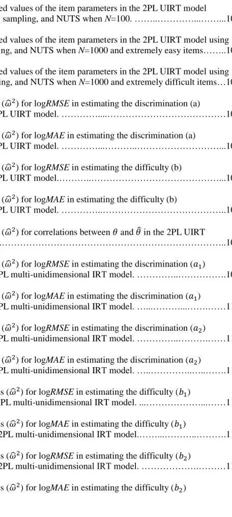
Figure 1 Trace plots of the discrimination parameterand difficulty parameter for one item in the 2PL UIRT model using Gibbs sampling (top) and NUTS (bottom). …..……… 49

Figure 2 Gelman-Rubin plots of the discrimination parameterand difficulty parameter for one

item in the 2PL UIRT model using Gibbs sampling (top) and NUTS (bottom). ……49

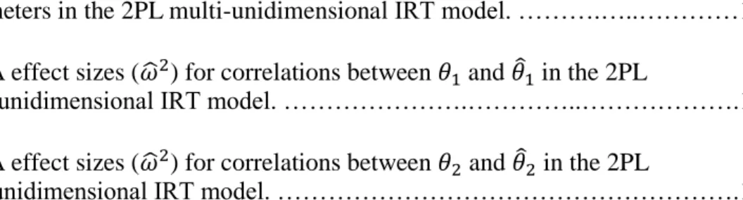
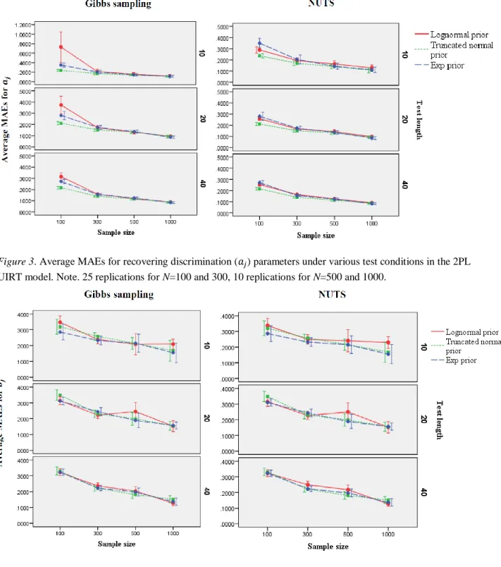
Figure 3 Average MAEs for recovering discrimination (𝑎_𝑗) parameters under various test

conditions in the 2PL UIRT model……….………..52

Figure 4 Average MAEs for recovering difficulty (𝑏𝑗) parameters under various test conditions

in the 2PL UIRT model….………52

Figure 5 Average correlations between the actual and estimated person abilities r(𝜃,𝜃̂) under

various test conditions for the 2PL UIRT model…..………56

Figure 6 Theinteractions ofsample size and prior specifications for 𝑎_𝑗 under different test

lengths in logRMSEa (left) and logRMSEb (right)…..………59

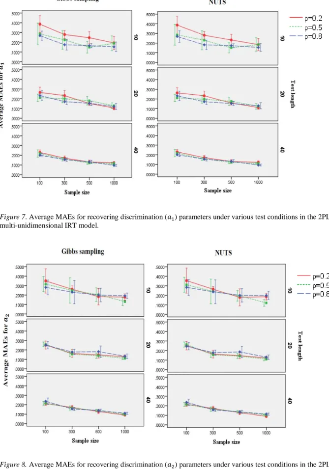
Figure 7 Average MAEs for recovering discrimination (𝑎₁) parameters under various test

conditions in the 2PL multi-unidimensional IRT model ……….62

Figure 8 Average MAEs for recovering discrimination (𝑎2) parameters under various test

conditions in the 2PL multi-unidimensional IRT model………..62

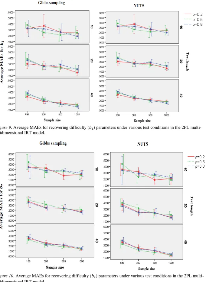
Figure 9 Average MAEs for recovering difficulty (𝑏₁) parameters under various test conditions

in the 2PL multi-unidimensional IRT model………63

Figure 10 Average MAEs for recovering difficulty (𝑏2) parameters under various test

conditions in the 2PL multi-unidimensional IRT model..………..63

Figure 11 Average correlations between the actual and estimated person abilities r(𝜃1,𝜃̂1) under

various test conditions for the 2PL multi-unidimensional model……….70

Figure 12 Average correlations between the actual and estimated person abilities r(𝜃2,𝜃̂2) under

various test conditions for the 2PL multi-unidimensional model……….……70

Figure 13 Theinteractions ofsample size and intertrait correlation under different test lengths

in logRMSE𝑎1 (left) and logRMSE𝑎2 (right)………...75

Figure 14 Theinteractions ofsample size and intertrait correlation under different test lengths

in logRMSE𝑏₁ (left) and logRMSE𝑏₂ (right)………...76

Figure 15 The probability density plot of lognormal(0, 0.5) distribution (left) and truncated

CHAPTER 1 INTRODUCTION

Educational and psychological measurement is a field of interest for many researchers to construct objective measurement of individuals’ skills, knowledge, and abilities. Classical test theory (CTT, Traub, 1997) is a psychometric theory that can be used to develop and further validate such measurement. The goal of CTT is to understand the characteristics of developed instruments, investigate the performance of individual items, and possibly improve the test’s reliability and validity. Although CTT has been broadly used in measurement for decades, it has its shortcomings. The major ones include (a) the person ability (e.g., observed scores) depends on items selected, and (b) the item characteristic (e.g., item difficulty or item discrimination) depends on groups selected (Hambleton & Swaminathan, 1985). Due to these, applications such as test equating and construction (Skaggs & Lissitz, 1986), computerized adaptive testing (CAT; Linden & Glas, 2000), differential item functioning (DIF; Holland & Wainer, 1993), linking and building item banks would be difficult to perform in CTT (Fan, 1998; Güler, Uyanık, & Teker, 2014). Item response theory (IRT; Lord, 1980), an extension of CTT, provides a solution. Instead of focusing on information at the test level as CTT does, IRT mainly postulates the probabilistic relationship between a person’s latent trait and the test at the item level. Latent traits are a specific type of constructs that refer to unobservable or unmeasurable objects. They include entities such as attitudes, preferences, and disposition and various underlying processes that educators are interested in measuring such as ability, aptitude, expertise, and intelligence. For example, we can use achievement tests to measure individuals’ constructs such as memory. Because of IRT’s advantages over CTT, it has gained increased popularity in large-scale

educational and psychological testing settings (e.g., Baker & Kim, 2004; De Ayala, 2009; Hambleton & Jones, 1993).

Based on the number of latent constructs being measured, IRT models can be conceived as being unidimensional or multidimensional. Unidimensional IRT (UIRT) models are utilized in circumstances when all test items measure one single latent trait. Dichotomous UIRT models (e.g., Birnbaum, 1969; Lord, 1980; Lord & Novick, 1968; Rasch, 1960) can be applied to

cognitive/achievement tests where two response categories such as correct/incorrect or true/false responses are used. Various such models have been developed in the literature, including the conventional one-, two-, and three-parameter models. The one-parameter model (Rasch, 1960; Wright & Stone, 1979) is the simplest IRT model because it only contains the difficulty

parameter (i.e., the ability required for individuals to have a probability of 50% to respond to the item correctly). The two-parameter model (Lord, 1952) extends the one-parameter model by adding the discrimination parameter, which is proportional to the slope at the point of the difficulty level. Items with steeper slopes are more useful for separating individuals with different ability levels than are items with less steep slopes. The three-parameter model extends the two-parameter model by adding the pseudo-guessing parameter, which is the probability of individuals with low ability answering the item correctly. With a logit or a probit link, these dichotomous UIRT models can be defined in either logistic or normal ogive forms. In the literature, such models are equivalent (Edelen & Reeve, 2007) in providing similar item characteristic curves (ICCs), which specify that as the level of latent trait increases, the probability of a correct response to an item increases (Hambleton, Swaminathan, & Rogers, 1991). Dichotomous UIRT models have been broadly studied in the literature (e.g. Kang & Cohen, 2007; Rizopoulos, 2006) and are the focus of this dissertation.

UIRT models have two major assumptions: unidimensionality and local independence (Lord, 1980). Unidimensionality states that only one single latent trait is measured by a set of

test items. This assumption is related to the assumption of local independence, which means that when the latent trait is held constant, individuals’ responses to any pair of items are independent. In other words, the latent trait measured by a test is the only factor that affects the probability of correct responses to individual items. In most situations, all test items are designed to measure one trait and hence it is appropriate to use UIRT models. However, when multiple traits are being measured or the test dimensionality structure is not obvious, using a UIRT model becomes problematic because measurement error inflates and incorrect inferences about an individual’s proficiency in a given subject may be made (e.g., Walker & Beretvas, 2000). In such cases, multidimensional IRT (MIRT; Reckase, 1997, 2009) models should be considered.

There are two general forms of MIRT models: compensatory and noncompensatory. For compensatory MIRT models, a lack of one trait dimension can be compensated by an increase of other trait dimensions (e.g., Ackerman, Gierl, & Walker, 2003; Reckase, 1985). However, for noncompensatory MIRT models, a lack of one cannot be offset by an increase of others (e.g., Sympson, 1978; Whitely, 1980). Due to the estimation complexity in noncompensatory MIRT models, most research has focused on compensatory MIRT models (De Ayala, 1992). By using the compensatory form, the multidimensional one-, two-, and three-parameter models can be extended from unidimensional models (De Ayala, 1992; DeMars, 2010). A special case of MIRT models is known as the multi-unidimensional IRT model when the overall test is multidimensional but each item measures only one latent trait (Sheng & Wikle, 2007).

To date, many estimation techniques have been developed for various IRT models with early focus being on using the joint maximum likelihood (JML; Birnbaum, 1969). The JML estimation begins with the joint probability (likelihood) of the item response vector given the person parameters. This procedure treats both item and person parameters as unknown and

simultaneously estimates them by maximizing the joint likelihood. The JML, however, tends to result in inconsistent and biased estimates (Andersen, 1970; Gruijter, 1990; Ghosh, 1995; Neyman & Scott, 1948).

The marginal maximum likelihood (MML; Bock & Aitkin, 1981) method based on the expectation maximization (EM) algorithm was developed in the early 1980’s to overcome the problems resulting from using the JML estimation. It treats persons as random effects and derives a marginal probability of observing the item response vector by integrating the person effects out of the joint likelihood in order to separate item parameters from person parameters. Therefore, in MML, two steps are taken where item parameters are first estimated using the EM algorithm after integrating out person parameters, and then person parameters can be

subsequently estimated by fixing the estimated item parameters as known. Given that both JML and MML produce estimators related to the maximum likelihood, they may result in either infinite or impossible parameter estimates in circumstances where unusual response patterns are observed (e.g., perfect or zero scores).

With the help of modern computer techniques, the estimation methods of IRT models have gradually shifted to the fully Bayesian estimation, which can simultaneously obtain posterior estimates for both item and person parameters. The fully Bayesian estimation via the use of Markov chain Monte Carlo (MCMC; Hastings, 1970) simulation techniques has

demonstrated its advantages over traditional maximum likelihood for IRT models (e.g., Kim, 2007; Mislevy, 1986; Swaminathan & Gifford, 1983). Unlike JML and MML, the Bayesian method can avoid unreasonable parameter estimates occurring. In addition, the Bayesian approach controls the parameters within a reasonable range via specifying appropriate prior distributions. Further, the fully Bayesian estimation, with the use of MCMC methods, is highly

flexible and has demonstrated its practical usefulness in all aspects of Bayesian inferences, such as parameter estimation or model comparisons.

As the name indicates, MCMC combines Monte Carlo with Markov chain. Monte Carlo is a computational simulation technique with the name coming from the Monte Carlo casino in Monaco. A Markov chain is a stochastic process that satisfies the Markov property if one can make predictions for the future process based solely on its present value. In other words, what happens next in the chain depends only on the current state of the system and not on how it reached the current state. An important feature of a Markov chain is its stationary distribution. The stationary state allows one to define the probability for every state of a system at a random time. Therefore, MCMC methods are a class of algorithms that can be used to simulate samples from a probability distribution via constructing a Markov chain that has the desired distribution (i.e., the posterior distribution) as its stationary distribution.

Common MCMC algorithms include Gibbs sampling (Geman & Geman, 1984) and Metropolis-Hastings (MH; Hastings, 1970; Metropolis & Ulam, 1949). These methods engage in random walk behaviors where at each step, the direction of the proposed move is random. If the relative probability of the proposed position is less than that of the current position, the acceptance of the proposed move is by chance. Due to the randomness, if the process were started over again, then the movement would certainly be different. Gibbs sampling is the simplest MCMC algorithm that requires the marginal distribution of each parameter conditional on the values of all the others to be in closed form. The algorithm works by drawing random samples of each parameter from its full conditional distribution based on the previously generated values of all the other parameters. Then, the joint posterior distribution can be

is not in closed form or is difficult to simulate, one has to use a more general MH algorithm, which chooses a proposal or candidate distribution by the current value of the parameters. Then, a proposal value is generated from the proposal distribution and accepted in the Markov chain with a certain amount of probability. Although the MH method can be applied in many situations, finding an appropriate proposal distribution for each parameter could sometimes be inefficient in the Markov chain. In addition, both Gibbs sampling and MH utilizing random walks have the general problem of possibly requiring too much time to reach convergence to the target distribution for complicated models with many parameters. These methods tend to explore the parameter space via inefficient random walks (Neal, 1992).

Other MCMC methods such as Hamiltonian Monte Carlo (HMC; Duane, Kennedy, Pendleton, & Roweth, 1987) and No-U-Turn Sampler (NUTS; Hoffman & Gelman, 2014) have been developed to avoid the random walk behavior that Gibbs sampling or MH exhibits by introducing an auxiliary momentum vector and implementing Hamiltonian dynamics so the potential energy function is the target density. HMC generates a proposal in a way similar to rolling a small marble on a hilly surface (the posterior distribution). The marble gains kinetic energy when it falls down the hill and earns potential energy when it climbs back up the hill. The proposed point is then accepted or rejected according to the Metropolis rule. HMC obtains a sequence of random samples from a probability distribution for which direct sampling is

difficult. This sequence can be used to approximate the distribution (i.e., to generate a

histogram), or to compute an integral (such as an expected value). NUTS further improves HMC by eliminating the need to manually set the number of steps in HMC at each iteration. The algorithm gets its name “no-U-turn” sampler because it prevents inefficiencies that would arise from letting the trajectories make a U-turn. NUTS generalizes the notion of the U-turn to high

dimensional parameter spaces and estimates when to stop the trajectories before they make a U-turn back toward the starting point. Gibbs sampling and NUTS can be implemented in software such as JAGS (Plummer, 2003) and Stan (Stan Development Team, 2016), respectively.

1.1Statement of the Problem

In the IRT literature, many studies have been conducted on the development and

application of Bayesian IRT models using Gibbs sampling or MH (e.g., Albert, 1992; Albert & Chib, 1993; Béguin & Glas, 2001; Patz & Junker, 1999a, 1999b; Sheng & Wikle, 2007, 2008, 2009) as well as using NUTS (Caughey & Warshaw, 2014; Zhu, Robinson, & Torenvlied, 2014). Also, studies comparing fully Bayesian and maximum likelihood estimation (MLE) have found that Gibbs sampling performs better than MH (e.g., Sahu, 2002) with the use of data

augmentation (Tanner & Wong, 1987) and MLE (e.g., Albert & Chib, 1993) with the small sample size situation. Recently, Grant, Furr, Carpenter, and Gelman (2016) tried to fit the one-parameter IRT model (Rasch, 1960) using both Gibbs sampling and NUTS. Although their results showed that NUTS performed better than Gibbs sampling, their study only focused on the computation speed and scalability. To date, no research has actually investigated the comparison of Gibbs sampling and NUTS in estimating the dichotomous UIRT and multi-unidimensional IRT models. Hence, given the increased popularity of fully Bayesian estimation using Gibbs sampling and NUTS, and the ease in implementing them via two computer programs, JAGS and Stan, it is important and necessary to investigate how these two types of MCMC algorithms perform in estimating item and person ability parameters in such models especially when different sample size, test length, prior specification, and/or intertrait correlation conditions for these IRT models are considered.

1.2Purpose of the Study

The purpose of the study is to evaluate the performances of two emerging MCMC algorithms, Gibbs sampling and NUTS, in estimating the two-parameter logistic (2PL) UIRT model and the 2PL multi-unidimensional IRT model under various test situations. The

parameter estimates were obtained using these two algorithms, which can be implemented in two computer programs, JAGS and Stan, respectively. The key motivation for this investigation is to provide researchers and practitioners with general guidelines when it comes to estimating a UIRT model and a multi-unidimensional IRT model using Gibbs sampling and NUTS. Moreover, the accuracy and bias in estimating the model parameters were investigated given different test lengths, sample sizes, prior specifications, or correlations for these models. 1.3 Research Questions

The general research question is to compare two types of MCMC algorithms, i.e., Gibbs sampling where random walk is utilized with NUTS where random walk behaviors are avoided for the 2PL IRT models. Each algorithm was implemented to the 2PL UIRT and

multi-unidimensional IRT models. The specific research questions related to the performance of the model and parameter estimations are as follows

1. How does Gibbs sampling compare with NUTS in estimating the 2PL UIRT model under

various test conditions where sample sizes, test lengths, and prior specifications differ?

2. How does Gibbs sampling compare with NUTS in estimating the 2PL

multi-unidimensional IRT model under various test conditions where sample sizes, test lengths, and intertrait correlations differ?

1.4 Definition of Terms

 Item response theory (IRT) − Item response theory, also known as the latent trait theory, is the theory used in educational and psychological measurement (e.g., achievement tests, rating scales, and inventories) that investigates a mathematical relationship between individuals’ abilities (or other mental traits) and item responses.

 Unidimensional IRT (UIRT) − UIRT assumes each of the individual trait level varies

continuously along a single dimension. A person’s response to a specific item is determined by a single unified latent trait.

 Multidimensional IRT (MIRT) − MIRT assumes multiple traits are measured by each

item.

 Multi-unidimensional IRT − It is a special case of MIRT. It assumes that an overall test

measures multiple latent traits, with each subtest measuring one of them. This implies that the overall test is multidimensional while each subtest is unidimensional. The latent traits can be correlated.

 Dichotomous IRT models − A dichotomous IRT model is used when a test involves

items with two response categories (e.g., true/false items).

 Fully Bayesian− It is a branch of mathematical probability theory that allows one to

model uncertainty about the world and outcomes of interest by combining common-sense (prior) knowledge and observational evidence (likelihood).

 Markov chain Monte Carlo (MCMC) − MCMC methods are a class of algorithms for

generating samples from a probability distribution via constructing a Markov chain that has the desired distribution as its stationary distribution. MCMC methods are used in data modeling for Bayesian inference and numerical integration.

 Random walk Monte Carlo methods – A MCMC algorithm can be a random walk that uses either an acceptance or rejection rule to converge to the target distribution.

Algorithms such as Gibbs sampling and Metropolis-Hastings algorithm are considered as random walk Monte Carlo methods.

 Gibbs sampling − This is one of the simplest MCMC algorithms. Gibbs sampling is

applicable when the joint posterior distribution is not known explicitly, but the conditional posterior distribution of each parameter is known. The idea of a Gibbs sampler is to obtain the joint posterior distribution by iteratively generating a random sample from the full conditional distribution for each parameter.

 Metropolis-Hastings (MH) − This is more general than Gibbs sampling and used when

any of the conditional posterior distributions do not have an obtainable closed form. The idea of MH is to generate a proposed value from a proposal distribution. Then the proposed value is accepted as the next value in the Markov chain with a certain probability.

 Hamiltonian Monte Carlo (HMC) −HMC is a MCMC algorithm that uses an auxiliary

momentum vector and implements Hamiltonian dynamics so the potential energy function is the target density.

 No-U-Turn Sampler (NUTS) – NUTS is one of the MCMC algorithms that build a set of

likely candidate points that span a wide swath of the target distribution, stopping automatically when it starts to double back and retrace its steps.

 JAGS – JAGS stands for just another Gibbs sampler and is a program for analysis of

Bayesian models with MCMC simulation using Gibbs sampling.

1.5 Significance of the Research

The significance of the study lies in the comparison between two MCMC algorithms for the 2PL dichotomous UIRT and multi-unidimensional IRT models under various test conditions. The results of the study provide researchers and practitioners with a set of guidelines on using Gibbs sampling and NUTS in estimating the two IRT models. Understanding the performance of the two algorithms for IRT models in various test situations would further provide guidance to future research when it comes to parameter estimation for IRT models using the algorithms under investigation. Findings from this study also provide empirical evidence on the use of Gibbs sampling or NUTS with more complicated IRT models.

1.6 Delimitation of the Study

The delimitations in this dissertation are described as follows.

1. This dissertation focuses on the two-parameter dichotomous IRT model. More item

parameters such as three-parameter IRT models, or polytomous IRT models such as the partial credit and the rating scale models are not considered.

2. This dissertation only compares two MCMC algorithms under the fully Bayesian

framework. Other MCMC algorithms such as Metropolis-Hastings or Hastings-within-Gibbs, or other estimation methods such as JML or MML are not considered.

3. When implementing the IRT models, this dissertation focuses only on simulated data not

real data because with simulations, the model parameters can be specified, which makes it possible to evaluate the performance of each estimation algorithm.

4. The two-parameter multi-unidimensional IRT model is a special case of the

corresponding MIRT model. It is noted that the multi-unidimensional model does not apply to situations where each item measures multiple latent traits.

5. The simulation study for the multi-unidimensional IRT model in this dissertation only considers situations where a test involves two subscales. The algorithms, however, can be applied to situations where more than two dimensions are involved.

1.7 Overview of Subsequent Chapters

The subsequent chapters are organized as follows. Chapter 2 reviews the related literature on the IRT models, estimation procedures, and the algorithms of implementing IRT models under the fully Bayesian framework. Chapter 3 describes the procedures of fitting the models with simulated datasets. Chapter 4 presents the results of simulation studies for the 2PL UIRT and multi-unidimensional IRT models. Finally, Chapter 5 summarizes the conclusion of findings, implication of this study, and the discussion for future research.

CHAPTER 2 LITERATURE REVIEW

The review of literature starts with the basic concept of item response theory. Five main sections are included in this chapter. The first section reviews the unidimensional and

multidimensional IRT models, with the multi-unidimensional model as a special case. The second section focuses on the estimation procedures with UIRT models. Section 3 reviews the estimation procedures with MIRT models. Section 4 concentrates on a few major Markov chain Monte Carlo (MCMC) algorithms and programs that can be used to implement these algorithms. The last section reviews prior research estimating unidimensional and multidimensional IRT models using fully Bayesian estimation via MCMC.

2.1 Item Response Theory

Item response theory (IRT; Lord, 1980) is a measurement theory used in educational and psychological assessments (e.g., achievement tests, rating scales, and inventories) that assumes a mathematical relationship between individuals’ abilities (or other mental traits) and item

responses (Baker & Kim, 2004; Hambleton et al., 1991; Wainer, Bradlow, & Wang, 2007). IRT is constructed on the concept that the probability of a correct response to an item is a

mathematical function of both person and item parameters (Hemker, Sijtsma, & Molenaar, 1995). It is generally considered as an improvement over classical test theory (CTT), which has become the norm for test measurement since the 1930s and has been the predominant

psychometric method with psychological instruments for most of the last century (Gulliksen, 1987). For tests that can be performed using CTT, IRT generally provides more flexibility and offers additional test information. Some applications, such as computerized adaptive testing (CAT), are enabled by IRT and cannot reasonably be performed using CTT only. Although CTT

has been used in educational and psychological measurement for decades, it has its own

limitations. For example, for CTT, the item characteristics are sample dependent, and hence can change based on the groups of individuals that are being selected. Another limitation of CTT is that the traits of individuals depend on the items selected. Thus, it is difficult to compare individuals’ latent traits if the test forms are not exactly parallel. IRT was developed to tackle the limitations of CTT and offered more information on test scores. IRT differs from CTT in that it has the property of invariance of item and latent trait characteristics, which indicates that the corresponding estimates are not sample or item dependent. In other words, latent trait

estimates from different item sets evaluating the same fundamental construct are similar and vary only because of the examinee measurement error. Item estimates from different respondent groups in the same population are similar and vary only because of the sampling error. The comparisons between IRT and CTT have been widely explored in the literature (see e.g., De Ayala, 2009; Hambleton & Jones, 1993; Thissen & Wainer, 2001).

2.1.1 IRT Major Assumptions

There are two main assumptions with conventional IRT models, including

unidimensionality and local independence. Unidimensionality states that only one single latent

trait 𝜃 is measured with a set of test items. In reality, this assumption can be difficult to meet

because several cognitive, personality, and test taking factors directly affect individuals’ test performance. To overcome this, a “dominant” factor that affects the test performance is

required. Once the assumption of unidimensionality is met, local independence is also obtained. To some extent, these two concepts are equivalent (Lord, 1980). Local independence means that when individuals’ latent traits are held constant, their responses to any pairs of items are

statistically independent. In other words, after taking individuals’ abilities into account, no relationship exists between individuals’ responses to test items.

Due to these assumptions, IRT models can be generally divided into two categories: unidimensional and multidimensional IRT models. Unidimensional IRT models assume each of

the latent traits varies continuously along a single dimension 𝜃, while multidimensional IRT

models are used to measure multiple traits (Reckase, 1997, 2009). However, given the greatly increased complexity involved with multidimensional IRT models, the majority of IRT research and applications focuses on unidimensional IRT models. In addition, based on the number of scored responses, IRT models can also be categorized as models for dichotomous outcomes (e.g., true/false; correct/incorrect), and those for polytomous outcomes, where each response has a different score value. A common example of the latter is Likert-type items (e.g., “Rate on a scale of 1 to 5”). Given that this dissertation focuses on dichotomous models, interested readers can refer to Samejima (1969, 1972), Masters (1982), and Muraki (1992) for polytomous models. 2.1.2 Unidimensional IRT (UIRT) Models

Common dichotomous UIRT models are described by the number of item parameters they consist of. The one-parameter model is the simplest UIRT model. The model contains an

item difficulty parameter (𝑏_𝑗), which corresponds to the ability required for individuals to

respond to the item correctly at a probability of 0.5. The one-parameter logistic (1PL) model, also known as the Rasch model (Rasch, 1960), is defined as the probability of a correct response

for person i to item j (𝑌_𝑖𝑗= 1):

P(𝑌_𝑖𝑗= 1|𝜃_𝑖, 𝑏_𝑗) = exp (𝜃𝑖−𝑏𝑗)

1+exp (𝜃_𝑖−𝑏_𝑗) , (2.1.1)

where 𝜃_𝑖 is the latent variable of person i (i = 1,…, N). 𝜃_𝑖 ranges from −∞ to +∞ and follows a

from −3 to 3 (DeMars, 2010). The range of 𝑏𝑗 (j = 1,…, K) is from −2 to 2 in practice when 𝜃𝑖

is assumed to be between −3 and 3 (Hambleton & Cook, 1977). Given that 𝑏_𝑗 denotes item

difficulty, the larger its value is, the more difficult this item becomes since it requires individuals’ greater ability to attain a 50% correct response. With a probit form, the one-parameter model can be defined as the one-one-parameter normal ogive model:

P(𝑌𝑖𝑗 = 1|𝜃𝑖, 𝑏𝑗) = Φ (𝜃𝑖− 𝑏𝑗), (2.1.2)

where Φ(∙) is the standard normal cumulative density function.

The two-parameter model assumes that items can vary in terms of difficulty (𝑏_𝑗) and

discrimination (𝑎𝑗). The two-parameter logistic (Lord & Novick, 1968) and normal ogive

models are defined as follows:

P(𝑌_𝑖𝑗= 1|𝜃_𝑖, 𝑎_𝑗, 𝑏_𝑗) = exp [𝑎𝑗(𝜃𝑖−𝑏𝑗)]

1+exp [𝑎_𝑗(𝜃_𝑖−𝑏_𝑗)] , and (2.1.3) P(𝑌_𝑖𝑗 = 1|𝜃_𝑖, 𝑎_𝑗, 𝑏_𝑗) = Φ[𝑎_𝑗(𝜃_𝑖− 𝑏_𝑗)], (2.1.4)

where 𝑎_𝑗 is referred to as the discrimination parameter for item j. The value of 𝑎_𝑗 can range from

−∞ to +∞, but in practice, it ranges from 0 to 2 (DeMars, 2010; Hambleton & Cook, 1977). An

item with a negative discrimination parameter suggests that individuals with greater abilities are less likely to answer the item correctly. Hence, such items should be revised or removed. The three-parameter model is an extension of the two-parameter model by adding a

pseudo-guessing parameter 𝑐_𝑗 for item j. The three-parameter logistic and normal ogive models

are described as

P(𝑌𝑖𝑗= 1|𝜃𝑖, 𝑎𝑗, 𝑏𝑗, 𝑐𝑗) = 𝑐𝑗+ (1 − 𝑐𝑗)

exp [𝑎_𝑗(𝜃_𝑖−𝑏_𝑗)]

1+exp [𝑎𝑗(𝜃𝑖−𝑏𝑗)] , (2.1.5) P(𝑌𝑖𝑗 = 1|𝜃𝑖, 𝑎𝑗, 𝑏𝑗, 𝑐𝑗) = 𝑐𝑗+ (1 − 𝑐𝑗) Φ[𝑎𝑗(𝜃𝑖− 𝑏𝑗)]. (2.1.6)

If a five-option multiple choice item is used, 𝑐𝑗 would be approximately 0.2, which is the chance

that an individual with an extremely low latent trait could answer this item correctly. For

example, in multiple-choice aptitude tests, even the least competent people can score by guessing

(Drasgow & Schmitt, 2002). For 𝑐_𝑗 > 0, the item difficulty is not the trait level at which the

probability that an individual answers correctly is 0.5. Instead, the inflation point (1+𝑐_𝑗)/2 is

shifted by the lower asymptote.

In summary, the three-parameter model gets its name because it contains three item

parameters, including the difficulty (𝑏𝑗), discrimination (𝑎𝑗), and guessing (𝑐𝑗) parameters. The

two-parameter model assumes that items can differ in terms of difficulty (𝑏𝑗) and discrimination

(𝑎_𝑗) with no guessing. The one-parameter model assumes that all items have comparable

discriminations and that guessing is a part of the ability, and hence items can be described by a

single parameter (𝑏_𝑗).

In addition to the three conventional IRT models, there is a hypothetically four-parameter

model (Barton & Lord, 1981), which adds an upper asymptote, represented by 𝑑𝑗. The upper

asymptote 𝑑_𝑗 allows high-ability students to miss an easy item without their ability being

drastically underestimated (Barton & Lord, 1981). Therefore, 1−𝑐𝑗 in the three-parameter model

is replaced by 𝑑_𝑗 − 𝑐_𝑗. This model, however, is rarely used. Note that the alphabetical order of

the item parameters does not necessarily suggest their practical or psychometric importance. The

difficulty parameter (𝑏𝑗) is clearly the most important because it is included in all four models.

The one-parameter model only has 𝑏_𝑗, the two-parameter model has 𝑏_𝑗and 𝑎_𝑗, the

The three-parameter model is equivalent to the two-parameter model with 𝑐𝑗 = 0, which is

appropriate for testing items where guessing the correct answer is highly unlikely, such as fill-in-the-blank questions (“What is the square root of 121?”), or where the concept of guessing does not apply, such as personality, attitude, or interest items (e.g., “Do you like Broadway musicals? Yes/No”).

2.1.3 Multidimensional IRT (MIRT) Models

When multiple latent traits are being measured or the test dimensionality structure is not obvious, it could be problematic to fit the data with a UIRT model since measurement error increases and incorrect inferences about an individual’s proficiency may be made (Walker & Beretvas, 2000). In such cases, multidimensional IRT (MIRT, Reckase, 1997, 2009) models should be used for dealing with this type of complicacy in educational and psychological measurement.

MIRT models have been developed to explain how test items interact with an individual when characteristics of an individual are defined using a vector of hypothetical constructs rather than a single unified trait (Reckase, 1997). The two most common MIRT models are

compensatory (e.g., Ackerman et al., 2003; Reckase, 1985) and non-compensatory (e.g., Sympson, 1978; Whitely, 1980) MIRT models. In compensatory MIRT models, a lack of one dimension can be compensated by an increase in other trait dimensions. For example,

individuals with a higher arithmetic problem-solving ability might be able to use it to

compensate for their lower algebraic symbol manipulation ability in order to correctly respond to a mathematical problem. In contrast, in non-compensatory multidimensional IRT models, a lack of one trait dimension usually cannot be compensated by an increase of others. For example, an individual with a very low reading proficiency attempts solving a math problem. Even with

extremely high mathematical skills, that individual will still be unable to solve the math problem described in words.

Due to the difficulties in estimation, more studies have focused on compensatory MIRT models rather than on non-compensatory models (De Ayala, 1992; Knol & Berger, 1991). For

example, in an m-dimensional test, the compensatory two-parameter logistic MIRT model can be

defined as (Reckase, 1985)

P(𝑦_𝑖𝑗=1|𝜽_𝑖, 𝜶_𝑗, 𝛾_𝑗) = logit(∑𝑚 𝑎_𝑣𝑗𝜃_𝑣𝑖− 𝛾_𝑗

𝑣=1 ) =

1

1+exp [−(∑𝑚_𝑣=1𝑎_𝑣𝑗𝜃_𝑣𝑖−𝛾_𝑗)] , (2.1.7)

where P(𝑦𝑖𝑗=1|𝜽𝑖, 𝜶𝑗, 𝛾𝑗) is the probability of a correct response of person i for item j, 𝜽𝑖=

(𝜃_𝑖1,…, 𝜃_𝑖𝑚)′ is an ability vector of person i for each of the m dimensions, 𝜶_𝒋 is a vector of

discrimination parameters where 𝜶_𝑗 = (𝛼_1𝑗,…, 𝛼_𝑚𝑗)′_{, and 𝛾}

𝑗 is a scalar parameter representing

the location in the latent space where the item is maximally informative. When the link function

is probit (Φ) rather than logit, the model is called the compensatory two-parameter normal ogive

MIRT model. The compensatory two-parameter logistic or normal ogive MIRT models are an extension of the two-parameter logistic or normal ogive UIRT models. Similarly, the

compensatory three-parameter logistic (normal ogive) MIRT models can also be extended from the three-parameter logistic (normal ogive) UIRT models (see De Ayala, 1992, for detailed descriptions and equations).

2.1.4 Multi-unidimensional IRT Model

The multi-unidimensional IRT model (Sheng & Wikle, 2007), also known as the

between-item MIRT model, can be considered as a special case of MIRT models. For the multi-unidimensional IRT model, items measure only one of the multiple latent abilities, which are commonly in the form of an overall test containing multiple unidimensional subsets or domains (e.g., de la Torre & Patz, 2005; Oshima, Raju, & Flowers, 1997; Sheng & Wikle, 2007; Wang,

Wilson, & Adams, 1997). For the multi-unidimensional IRT model, the vector of discrimination

parameters in the MIRT model as defined in (2.1.7) is simplified to 𝜶_𝑗 = (0,…, 0, 𝛼_𝑣𝑗, 0, … ,0)′_.

Specifically, suppose a K-item test containing m subtests, each having 𝑘𝑣 multiple-choice items

that measure one trait dimension. With a logit link, the probability of person i obtaining a

correct response for item j of the vth subtest can be defined as follows (Lee, 1995):

P(𝑦_𝑣𝑖𝑗 = 1|𝜃_𝑣𝑖, 𝛼_𝑣𝑗, 𝛾_𝑣𝑗) = logit (𝛼_𝑣𝑗𝜃_𝑣𝑖− 𝛾_𝑣𝑗) = 1

1+exp [−(𝛼𝑣𝑗𝜃𝑣𝑖−𝛾𝑣𝑗)] , (2.1.8)

where 𝛼𝑣𝑗 and 𝜃𝑣𝑖 are scalar parameters representing the item discrimination and the examinee

ability in the vth ability dimension, and 𝛾_𝑣𝑗 is a scalar parameter indicating the location in that

dimension where the item provides maximum information. With a probit link, the two-parameter normal ogive multi-unidimensional IRT model can be defined as

P(𝑦𝑣𝑖𝑗 = 1|𝜃𝑣𝑖, 𝛼𝑣𝑗, 𝛾𝑣𝑗) = Φ (𝛼𝑣𝑗𝜃𝑣𝑖− 𝛾𝑣𝑗) = ∫ 1 √2𝜋𝑒 −𝑡2 2 𝑑𝑡 𝛼_𝑣𝑗𝜃_𝑣𝑖−𝛾_𝑣𝑗 −∞ . (2.1.9)

2.2 Parameter Estimation of UIRT Models

Accurate recovery of model parameters from response data is a central problem in the IRT models. In fact, successful applications of IRT highly rely on finding appropriate

procedures for estimating the model parameters (Hambleton et al., 1991). Numerous estimation techniques have been developed for various IRT models in the past decades. The early method focused on using joint maximum likelihood (JML) and conditional maximum likelihood (CML) estimations. The problem with estimating the item parameters using JML was its tendency to obtain inconsistent estimators (Andersen, 1973). Compared with JML, CML produced more consistent and efficient parameter estimates by removing the trait level parameters from the likelihood equations (Si & Schumacker, 2004). However, when applying the CML estimation to the Rasch model, the parameter estimates are inconsistent due to the loss of item information

from the marginal distribution (Andersen, 1973). Bock and Aitkin (1981) presented an

algorithm based on the expectation maximization (EM) and since then, the standard approach has been the marginal maximum likelihood (MML) estimation. Modern computer technologies also helped the development of parameter estimation (see Zhao & Hambleton, 2009, for a comparison of the current computer software for IRT analysis) and made it possible to move to the fully Bayesian estimation (e.g., Chib & Greenberg, 1995). Lord (1980) and Baker and Kim (2004) provided a comprehensive review of the methods for parameter estimation with UIRT models. Three main estimation methods, including the JML, MML, and Bayesian estimation are

reviewed as follows.

2.2.1 Joint Maximum Likelihood (JML)

The joint maximum likelihood (JML) method relies on the assumption of local independence that individuals’ traits are independent of one another and item responses of an

individual are independent given the individual’s trait 𝜃𝑖. Therefore, the joint probability

(likelihood) of the person parameter 𝜃_𝑖 given 𝒚_𝑖is

L(𝜃𝑖|𝒚𝑖, 𝝃) = P(𝒚𝑖|𝜃𝑖, 𝝃) = ∏𝑘𝑗=1𝑃(𝒚𝑖𝑗|𝜃𝑖,𝝃𝑗), (2.2.1)

where 𝝃_𝑗 is the vector of all item parameters for item j in the IRT model. For example, for the

unidimensional two-parameter logistic (2PL) model, 𝝃𝑗 = (𝑎𝑗, 𝑏𝑗)′ and the likelihood for 𝜃𝑖 is

L(𝜃_𝑖|𝒚_𝑖, 𝝃) = exp {𝜃𝑖∑ 𝑦𝑗 𝑖𝑗𝑎𝑗−∑ 𝑦𝑗 𝑖𝑗𝑎𝑗𝑏𝑗}

∏ (1+exp{𝑎_{𝑗 𝑗}(𝜃_𝑖−𝑏_𝑗)}) . (2.2.2)

The JML method maximizes the joint likelihood function in equation (2.2.1) via simultaneously estimating both item and person parameters. The method treats both item and individual

parameters as unknown so the model is unidentified. Therefore, there is no unique solution to find the maximization. To overcome this, constraints have to be placed on the parameters of the model in order to ensure the existence of a solution. Even with constraints, the problem is that

the maximization equation cannot be solved analytically unless a numerical method is used. Another problem with the JML method is that the estimations could be inconsistent (Andersen, 1970; Ghosh, 1995; Neyman & Scott, 1948). This is because a limited number of item

parameters are estimated in the presence of many person parameters. In that case, regardless of how many individuals are included in the data, the estimation of the item parameters may still be biased (Gruijter, 1990). The JML method is implemented in the LOGIST (Wingersky, 1992) software for one-, two-, and three-parameter IRT models.

2.2.2 Marginal Maximum Likelihood (MML)

The marginal maximum likelihood (MML) method takes a different approach to

eliminate the problems encountered in the JML method by treating individuals as random effects and separating person parameter estimation from item parameter estimation via estimating item

parameters first. In MML, it is assumed that person parameters 𝜃_𝑖 are random effects sampled

from a large continuous distribution, denoted F(𝜃). The marginal probability of observing the

item response vector 𝒚𝐢 is derived by integrating the random person effects out of the joint

likelihood defined in (2.2.1), i.e.,

P(𝒚i| 𝝃) = ∫ 𝐿(𝜃_𝜃𝑖 𝑖|𝒚𝑖, 𝝃)𝑑𝐹(𝜃𝑖). (2.2.3)

Taking the product of the probabilities in (2.2.3) over individuals i defines the marginal

likelihood of the item parameter vector 𝝃:

L(𝝃|y) = ∏ 𝑃(𝒚_{𝑖 𝑖}|𝝃). (2.2.4)

The MML estimates for the item parameter 𝝃 can be acquired by maximizing the marginal

likelihood in (2.2.4) using the EM algorithm. Then, the person parameters 𝜃_𝑖 can be obtained

using the item parameter estimates. Like the JML method, constraints are needed to identify the model. The constraints can either be placed on the mean and standard deviation of the

propensity distribution F or on the item parameters. Typically, the distribution F is assumed to be the standard normal distribution, but the normal distribution does not necessarily work for all

situations. Therefore, it becomes difficult to specify the distribution F (Johnson, 2007). In

addition, both JML and MML methods encounter the problems that they may result in infinite or impossible parameter estimates. The MML method is directly implemented in BILOG-MG (Zimowski, Muraki, Mislevy, & Bock, 2003) for the one-, two-, and three-parameter logistic IRT.

2.2.3 Bayesian Estimation

In the IRT literature, the Bayesian estimation includes a marginal Bayes and a fully Bayesian method. Generally speaking, in the Bayesian approach, model parameters are considered random variables and have prior distributions that reflect the uncertainty about the true values of the parameters before observing the data. The item response models discussed for the observed data are referred to as likelihood models and are the part of the model that presents the density of the data conditional on the unknown model parameters. Therefore, two modeling stages can be recognized: (1) the specification of a prior and (2) the specification of a likelihood model. After observing the data, the prior information is combined with the information from the data and a posterior distribution is constructed. Bayesian inferences are made conditional on the data, and inferences about parameters can be made directly from their posterior densities. The marginal Bayes estimation uses similar ways for estimating IRT models as the MML method, but the difference is that it places a prior distribution for each parameter in the model. For example, in the three-parameter logistic (3PL) model, the discrimination parameter can be specified to follow a log normal distribution, the difficulty parameter is specified to follow a normal distribution, and the guessing parameter can follow a beta distribution. Then, with

information from data (the likelihoods), posterior estimates of item parameters (usually in the form of the mode of the posterior distribution) can be obtained using these priors.

On the other hand, the fully Bayesian estimation can simultaneously obtain posterior estimates for both item and person parameters, and can find the mean of the posterior

distribution. Wollack, Bolt, Cohen, and Lee (2002) suggested that fully Bayesian estimation provides a solution when the MML method is not applicable. For decades during the early stage of the development of IRT, the fully Bayesian estimation was not computationally practical for models with a very large number of parameters such as IRT models and therefore, the MML and the marginal Bayes have been the standard estimation methods. Modern computational

technology and the development of Markov chain Monte Carlo (MCMC; Hastings, 1970; Metropolis, Rosenbluth, Rosenbluth, Teller, & Teller, 1953; Metropolis & Ulam, 1949) algorithms, however, have made the fully Bayesian estimation applicable to fit different IRT models (e.g., Béguin & Glas, 2001; Bolt & Lall, 2003; Bradlow, Wainer, & Wang, 1999; de la Torre, Stark, & Chernyshenko, 2006; Fox & Glas, 2001; Johnson & Sinharay, 2005; Patz & Junker, 1999a). MCMC methods are a class of algorithms for sampling from a probability distribution (e.g., the posterior distribution) based on constructing a Markov chain that has the desired distribution as its stationary distribution. At each state of the Markov chain, random samples of model parameters are generated from the distribution based on those generated from a previous state. Since early samples may be affected by initial values, they are discarded in the so-called burn-in stage. After the burn-in stage, the quality of the sample becomes

approximately stable. Different MCMC algorithms have been developed in the last two decades, and a review of the major ones is made in a later section of this chapter. MCMC methods have been proven useful in practically all aspects of fully Bayesian inference, such as parameter

estimation and model comparisons. Albert (1992) was the first to apply the fully Bayesian estimation with IRT by fitting the two-parameter normal ogive (2PNO) IRT model using an MCMC algorithm. Since then, other UIRT models have been developed under the fully Bayesian framework such as two- and three-parameter logistic models (Patz & Junker, 1999a, 1999b) and three-parameter normal ogive models (Sahu, 2002).

Many studies have demonstrated advantages of Bayesian estimation, including the marginal Bayes and the fully Bayesian estimation, over MML and JML methods (e.g., Kim, 2007; Mislevy, 1986; Swaminathan & Gifford, 1983; also see Appendix A for a demonstration of the advantages of fully Bayesian estimation over MML). For example, with the specified prior distribution of item parameters, the Bayesian method avoids the possibility of having unreasonable parameters using MML and JML methods. The specified priors can pull extreme estimates back toward the center of their respective distributions and stop them from assuming unreasonable values. This effect should be more noticeable for small samples and short tests (e.g., Lim & Drasgow, 1990). Even with larger samples and longer tests, however, Bayesian estimation is still superior to JML and MML methods when unusual response patterns occur. For example, individuals may answer all items correctly or incorrectly, or they may answer easy items incorrectly while answering difficult items correctly. Under these circumstances, JML and MML methods would not be able to find an estimate while the Bayesian method will still

estimate the parameters within a reasonable range (Baker, 1987; Swaminathan & Gifford, 1983). The fully Bayesian method also has advantages over the marginal Bayes estimation.

Specially, in the marginal Bayes method, person parameters 𝜃_𝑖 are treated as random variables

and integrated out from the joint likelihood of item and person parameters. However, when the

to implement marginal Bayes. On the other hand, the fully Bayesian approach circumvents the

problem of integrating out 𝜃_𝑖 since it simultaneously draws samples from the posterior

distributions of model parameters.

2.3 Parameter Estimation of MIRT Models

The estimation procedures for MIRT models are relatively complicated for the following reasons (Reckase, 2009). First, as with UIRT, the models contain both person and item

parameters and generally, it is difficult to estimate the two sets of parameters independent of each other. Second, compared to UIRT models, MIRT models have more parameters that need to be estimated and hence are more complex. A third reason is that there are indeterminacies in the models such as the location of the origin of the space, the units of measurement for each coordinate axis, and the orientation of the coordinate axes relative to the locations of the persons. All of these issues must be addressed in the construction of an algorithm for estimating the

model parameters.

Bock and Aitkin (1981) developed an EM algorithm (Dempster, Laird, & Rubin, 1977) to estimate the parameters of the one-, two-, and three-parameter normal ogive MIRT models for dichotomous items. The algorithm, however, is limited to small testing situations (Baker & Kim, 2004) and it does not work well with a large number of dimensions, either. More estimation methods and computer software have subsequently been developed using the MML technique. For example, Bock, Gibbons, and Muraki (1988) used the MML method and EM algorithm for dichotomous MIRT models and discussed technical problems of its implementation for a number of simulated and real datasets. TESTFACT (Wilson, Wood, & Gibbons, 1991) is a computer program that can be used to implement a nonlinear, exploratory factor analysis for dichotomous test items. The program uses the MML method with an EM algorithm to estimate item

parameters in the MIRT model. Then, person parameters are estimated using the Bayesian method by fixing the item parameters.

Trying to use the MML method for MIRT models has been impeded by the fact that the computations involve a numerical integration over the latent ability distribution. With an increased dimensionality, the ability is a multivariate distribution involving more parameters. This makes integration to be computationally demanding such that the applicability of higher dimensional IRT models is impossible in practical settings (Rijmen, 2009). Therefore, more and more researchers have resorted to the fully Bayesian estimation for MIRT models. For example, the algorithm introduced by Albert (1992) for the unidimensional two-parameter normal ogive model was extended to the dichotomous MIRT models (Béguin & Glas, 2001). Other

applications of Bayesian estimation of multidimensional dichotomous IRT models can be seen in various studies (e.g., Lee, 1995; Sheng & Headrick, 2012; Sheng & Wikle, 2007, 2008, 2009; Yao & Boughton, 2007; Zheng, 2000).

2.4 MCMC Algorithms

The concept of MCMC methods is to generate samples from a probability distribution via constructing a Markov chain that has the desired distribution as its stationary distribution. As the name shows, MCMC starts with Monte Carlo, a computational simulation technique with a catchy name, i.e., the Monte Carlo casino in Monaco. A Markov chain is a sequence of random

variables, {𝑋₀, 𝑋₁, 𝑋₂,…}, sampled from the distribution p(𝑋_𝑘+1|𝑋_𝑘). Then, each subsequent

sample 𝑋_𝑘+1 depends on the current state 𝑋_𝑘 rather than on previous history {𝑋₀, 𝑋₁, 𝑋₂,…,

𝑋𝑘−1}. An important concept of a Markov chain is its stationary distribution. The stationary

state allows one to define the probability for every state of a system at a random time. Under the fully Bayesian framework, MCMC methods are a class of algorithms that can be used to simulate

samples from the posterior distribution and these posterior samples can then be used to summarize the posterior distribution.

Using MCMC-based fully Bayesian methods for estimating complex psychometric models such as IRT models has become popular in recent years. These sampling based methods are more flexible and can provide a more complete picture of the posterior distribution of all parameters in the model than JML or MML does. They can be applied in situations (e.g., small sample size) where the likelihood methods fail or are difficult to implement. The samples produced by the MCMC procedure can also be used for conducting model fit diagnosis, model selection, and model-based prediction.

Common MCMC methods are performed under the notion of random walks, which imply that at each step, the direction of the proposed move is random. If the relative probability of the proposed position is more than that of the current position, then the proposed move is always accepted. If the relative probability of the proposed position, however, is less than that of the current position, the acceptance of the proposed move is by chance. Due to the randomness, if the process were started over again, then the movement would certainly be different. However, regardless of the specific movement, in the long run the relative frequency of visits will be close to the target distribution. The random walk nature of the algorithms can greatly increase the number of iterations required before convergence is reached and/or the number of subsequent iterations that are needed to gather a sample of states from which accurate estimates for the quantities of interest can be obtained. To overcome such inefficiency, other MCMC algorithms such as Hamiltonian Monte Carlo (HMC; Duane et al., 1987) have been developed to reduce random walk behaviors. These algorithms are reviewed as below.