Title of Thesis: Interactive Illumination Using Large Sets of Point Lights
Name of Candidate: Joshua David Barczak
Master of Science, 2006
Thesis and Abstract Approved: _________________________________________
Marc Olano
Assistant Professor
Dept. of Computer Science and Electrical
Engineering
Curriculum Vitae
Name:
Joshua Barczak
Permanent Address:
14 S. Belle Grove Rd, Apt. B. Catonsville, MD 21228
Degree and Date Conferred:
Master of Science, 2006
Date of Birth:
July 22, 1981
Place of Birth:
Baltimore, MD
Secondary Education:
Perryville High School
Perryville, MD
Graduated May 1999
Collegiate Institutions Attended:
University of Maryland, Baltimore County. Master of Science. 2006
University of Maryland, Baltimore County. Bachelor of Science. 2003
Major: Computer Science
Professional Publications:
NEHAB, D. BARCZAK, J. SANDER, P. 2006. Triangle Order Optimization
for Graphics Hardware Occlusion Culling. Proceedings of the SIGGRAPH 2006
Symposium on Interactive 3D Graphics and Games (to appear)
Professional Positions Held:
Research Intern ATI Research, Inc. Marlborough, MA (June-August 2005)
Research Intern. ATI Research, Inc. Santa Clara, CA (June-August 2004)
Title of Thesis:
Joshua Barczak, Master of Science, 2006
Thesis Directed by: Marc Olano, Assistant Professor, Computer Science and
Electrical Engineering
There are a number of techniques in the field of computer graphics in which the illumination in a scene is approximated by a set of point light sources. These techniques are not well-suited to interactive applications, because evaluating the contribution of large sets of point lights can require a great deal of computation.
In this work we present an approach to rendering scenes containing large numbers of lights, using programmable graphics hardware. Our approach uses a geometric visibility determination algorithm in order to avoid performing visibility computation at the pixel level. In addition, by pre-computing and storing visibility information, and amortizing the update cost over several frames, we are able to support scenes containing moving objects.
We apply our techniques to the problems of rendering soft shadows from area light sources, and diffuse indirect illumination, and are able to render screen-sized images of scenes with several hundred lights at interactive speeds. Our optimization techniques allow us to render a significantly larger number of shadowed point lights than previous interactive systems. We present experimental results showing a significant performance improvement over a more straightforward baseline implementation.
Interactive Illumination Using Large Sets of Point
Lights
By.
Joshua David Barczak
Thesis submitted to the Faculty of the Graduate School of the University of Maryland in
partial fulfillment of the requirements for the degree of Master of Science 2006
Acknowledgements
Thanks to my parents for their continued love and support, especially to my father, for
proofreading this entire thing.
Thanks to my fiancée for her constant encouragement, and for not tolerating any
procrastination.
Table Of Contents
1 Overview... 1
2 Background... 4
2.1 Graphics Hardware ... 4
2.1.1 Modern GPU Architectures ... 4
2.1.2 Programmable Shaders... 7
2.2 Global Illumination... 8
3 Related work ... 11
3.1 Classical Global Illumination Algorithms... 11
3.2 Shadowing Algorithms... 13
3.3 Global Illumination in Interactive Applications... 15
3.4 Instant Radiosity ... 16
4 Method... 18
4.1 Light Sample Generation ... 18
4.2 Shadow Mapping ... 19
4.2.1 Shadow Map Parameterization ... 20
4.2.2 Shadow Map Rendering ... 22
4.3 Rendering Illuminated Scenes... 23
4.3.1 Visibility Determination ... 24
4.3.2 Light Mapping... 26
4.3.3 Lowres Pass... 27
4.3.4 Multi-pass Rendering implementation... 28
4.3.5 Render Pass Optimization... 30
4.4 Rendering Complex Meshes ... 33
4.4.2 Limitations of PRT... 35
4.5 Handling Dynamic Objects ... 36
4.5.1 Updates to Visibility Information ... 36
4.5.2 Light maps... 38
4.5.3 Shadow Maps ... 38
5 Results... 40
5.1 Static Scene Performance... 40
5.2 Dynamic Scene Performance ... 42
5.3 Direct Illumination Quality ... 44
5.4 Indirect Illumination Quality... 47
6 Conclusions, Limitations and Future Work... 49
6.1 Limitations of Instant Radiosity... 49
6.2 Improving Scalability... 51
6.3 Dynamic Light Sets... 51
List of Figures
Figure 1-1 ... 2 Figure 1-2 ... 2 Figure 1-3 ... 3 Figure 2-1 ... 5 Figure 3-1 ... 13 Figure 4-1 ... 20 Figure 4-2 ... 20 Figure 4-3 ... 21 Figure 4-4 ... 22 Figure 4-5 ... 25 Figure 4-6 ... 25 Figure 4-7 ... 27 Figure 4-8 ... 28 Figure 4-9 ... 30 Figure 4-10... 31 Figure 4-11... 32 Figure 4-12... 32 Figure 4-13... 34 Figure 4-14... 35 Figure 4-15... 36 Figure 4-16... 39 Figure 5-1 ... 41 Figure 5-2 ... 41Figure 5-3 ... 42 Figure 5-4 ... 42 Figure 5-5 ... 43 Figure 5-6 ... 44 Figure 5-7 ... 45 Figure 5-8 ... 46 Figure 5-9 ... 47 Figure 5-10... 48 Figure 6-1 ... 50 Figure 6-2 ... 51
List of Tables
1 Overview
Although the field of computer graphics has had great success in rendering plausible illumination in interactive applications, the quality of the illumination leaves much to be desired. Interactive computer graphics still struggles with the problem of reproducing global illumination effects, in which the objects in the scene influence each other’s appearance by changing the amount of light that reaches the surfaces. One important example is the state of shadow rendering. Modern interactive applications can render direct shadows from a small number of point light sources, but the shadows that are produced typically have rigid, geometric edges. These types of shadows are often referred to as “hard” shadows. In real scenes, most shadows are “soft”, and exhibit a gradual transition from light to dark regions (see Figure 1-1).
Figure 1-1 : Direct illumination with hard shadows (left) and soft shadows (right).
Indirect illumination is another effect which is important in real life, but which is typically badly approximated in interactive applications. Indirect illumination occurs when a surface is illuminated by light that is first reflected by another surface, rather than emitted directly from the source. Much of the illumination that humans observe is indirect, especially in indoor environments. The traditional (and least correct) solution to the indirect illumination problem is to add a constant term to every illumination computation to take into account the “ambient” illumination in the environment. This is often better than ignoring indirect illumination, but the results are obviously inaccurate, especially when compared to a rendering which better approximates the indirect illumination (Figure 1-2). In static environments, illumination can be pre-computed using a global illumination algorithm and used to render interactive walkthroughs (light mapping), but this method is only correct if light sources and objects remain in a fixed configuration. In scenes with moving objects, light mapping will be inaccurate. Many interactive applications, especially games, use light mapping for static geometry such as walls, and less accurate techniques for characters and moving objects.
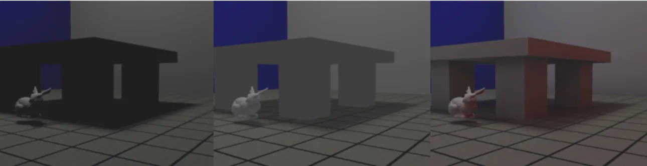
Figure 1-2 : A scene rendered with direct illumination (left), constant ambient illumination (middle), and our method (right). The red light in the right image is due to reflection from a red
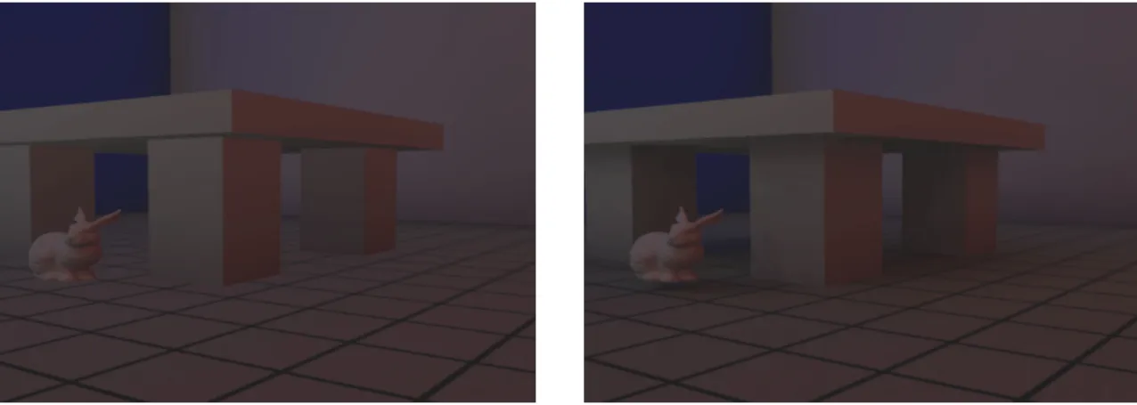
Indirect illumination computations are especially problematic if occlusion is to be considered. Although some previous work has chosen to ignore shadowing in indirect illumination, we believe that its effect is far too important to ignore, as shown in Figure 1-3.
Figure 1-3 : A scene rendered with only indirect illumination. Left: Without occlusion. Right: With Occlusion.
In this master’s thesis, we present a rendering system which is able to handle soft shadowed direct illumination, and indirect illumination with occlusion, while rendering at interactive rates. We accomplish this by adapting the instant radiosity algorithm [Keller 1997] to run efficiently on modern programmable graphics hardware. Our solution to the problems of indirect illumination and soft shadows is to simply apply standard direct illumination techniques on a large scale. We employ a number of optimization techniques which allow us to achieve an order of magnitude speedup over a naïve, brute force implementation for scenes with several hundred lights. We are able to support moving objects, to some extent, by carefully limiting the amount of re-computation that is performed in response to a change in the scene, and by amortizing the cost over multiple frames.
The remainder of this thesis is organized as follows: Chapter 2 describes the capabilities of programmable graphics hardware, and provides a primer on global illumination. Chapter 3 provides a review of relevant prior work. Chapter 4 describes the techniques employed in our rendering system. Chapter 5 provides an analysis of our rendering performance and image quality. Chapter 6 describes the limitations of the current system and suggests avenues for futures work.
2 Background
We begin by presenting a basic introduction to the capabilities of modern graphics hardware. We then give a brief description of global illumination, as it is understood in computer graphics. We describe the classical global illumination algorithms, and recent attempts to accelerate global illumination techniques using graphics hardware.
2.1 Graphics Hardware
In this section, we present a brief, high-level overview of the capabilities of modern graphics accelerators (GPUs). We begin by giving a high-level description of the rendering pipeline that is implemented by modern GPUs, such as the NVIDIA GeForce 5900 or 6800 series, or the ATI Radeon X800 or X1800 series. We then discuss the user-programmable portions of the pipeline in more detail, and present an overview of the programming model that is exposed by graphics APIs such as DirectX.
2.1.1 Modern GPU Architectures
Commercial graphics accelerators use specially designed hardware to produce images by rendering lines or polygons using a scanline rendering (rasterization) algorithm. The rendering pipeline that these accelerators implement can be
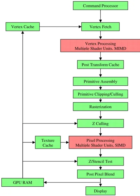
broken down into several stages, some of which are user-programmable. In the first stages, polygon vertices are fetched from GPU memory, and are transformed to align the polygons to a particular viewpoint and account for perspective. In addition to the transformation of vertex positions, other computations such as animation or lighting are sometimes performed at this stage, using additional information that is stored with the vertex positions. On modern graphics accelerators, there are generally a number of floating-point vector processors which perform vertex processing in a MIMD fashion. Modern accelerators also contain a dedicated cache to store the results of the computation for several previous vertices, allowing redundant computation to be skipped if vertices in a model are repeated (as they often are).
Figure 2-1: The rendering pipeline implemented by a modern GPU. Components colored green are implemented using fixed hardware. Components colored red are user-programmable.
Primitive Clipping/Culling Rasterization Vertex Processing Multiple Shader Units, MIMD
Primitive Assembly Post Transform Cache
Pixel Processing Multiple Shader Units, SIMD Texture
Cache
GPU RAM
Z Culling
Z/Stencil Test Post Pixel Blend
Vertex Fetch Vertex Cache
Command Processor
After vertex processing, the vertices of each triangle are collected and passed to dedicated rasterization hardware, which is responsible for determining the set of pixels covered by a given primitive. In addition to positions, additional values such as colors, surface normals, and texture coordinates can be generated for each vertex by the vertex processors, and interpolated between the vertices as the pixels of the polygon are plotted. Modern hardware is typically able to interpolate up to thirty-two floating-point values, organized as eight four-component vectors, in addition to the vertex position. Prior to rasterization, polygons which are only partly visible have their invisible portions discarded, through a process called clipping. In addition, polygons which are completely outside the screen area, or which face away from the viewer, are detected and discarded. In addition to the fixed-function clipping and culling, modern hardware allows the user to specify user-defined clipping planes, which can be used to clip geometry in a variety of ways. We make use of these clipping planes during our shadow map rendering.
After rasterization, additional computation must be performed for each rasterized pixel in order to determine its final color. Most of the transistors in modern GPUs are dedicated to pixel processing. Pixel-processing is carried out by a set of vector processors (between 12 and 24 on current models), which operate on blocks of pixels in a SIMD fashion. The pixel processors can perform arbitrary computations using the interpolated outputs of the vertex processors, and can also access additional data by reading pixels from a set of images known as texture maps. Texture maps are blocks of image data which can be stored in a variety of formats. This functionality is typically used to map images onto a polygon in order to add fine detail to the scene. For example, a surface which represents a wall may have a brick image mapped onto it. There are a myriad of other uses for texture mapping, such as storing illumination values (light mapping) or applying detailed, small-scale displacements to a surface (bump mapping). Modern graphics hardware typically supports a variety of filtering operations on texture data in order to eliminate certain kinds of artifacts that can occur in the image, but filtering is generally not supported on all texture formats.
In addition to rasterization, graphics hardware must also perform hidden surface elimination, in order to ensure that polygons which overlap on the screen are properly occluded, regardless of the order in which they are drawn. This is accomplished by using a technique called Z-buffering. A screen-aligned buffer is used to store a depth value for each pixel, which represents the distance from the eye to the point on the nearest polygon. The depth value is a function of the Z-component of the pixel’s position, relative to the camera. When a pixel is plotted, its depth value is compared to the depth value currently in the Z-buffer, and if its depth value is higher, the pixel is discarded. On modern graphics hardware, the Z test can usually be performed early, prior to pixel processing, which allows the potentially expensive pixel processing operations to be skipped for occluded pixels. Current GPUs also employ hierarchical Z buffering techniques [Green et al. 1993, Xi and Schantz 1999] which allow them to efficiently discard occluded pixels during rasterization.
In addition to the Z-buffer, modern accelerators offer an additional buffer which is known as the stencil buffer. The name is derived from the fact that the intended use of this functionality was to mask out pixels which are covered by user-interface elements, and which should not be modified when rendering a frame. The stencil buffer is essentially a single-byte counter for each pixel, which can be set to automatically increment or decrement whenever a pixel is plotted in the given location. In addition, a test can be specified for the stencil value to disable writing to pixels under certain conditions. The most common use of this functionality is for shadow rendering, using the shadow volume technique [Heidmann 1991, Everett and Kilgard 2002], but it can be used for a variety of other purposes. Stencil testing occurs immediately after Z testing, and the stencil bits are often stored in the same memory word as the depth buffer bits (using 24 bits for depth and eight for stencil).
After pixel processing, a variety of post-processing operations are available which can be used to combine the colors of the resulting pixel with the colors already in the render target. This post-processing stage is commonly referred to as the alpha-blending stage, because it is most often used to implement transparency by using an ‘alpha’ term to interpolate between two colors. Alpha blending can also be used to sum the results of several rendering passes, or to modulate one set of pixel values by another.
After post-processing, the final values for all pixels are written into a fixed location in GPU memory (the exact location is determined by the rasterization process). Current graphics accelerators do not have the ability to perform so-called “scatter” writes, in which a shader unit writes to an arbitrary memory location. In addition to writing to the frame buffer that is used to drive the display, modern hardware can also write pixels to a texture map, so that the results of the computation can be used in subsequent rendering operations.
2.1.2 Programmable Shaders
During the past few years, the flexibility of commercial GPUs has been significantly increased by the advent of user-programmable architectures. Modern graphics APIs such as DirectX or OpenGL expose this functionality to application developers by providing an interface to supply user-defined programs (shaders), written in a special-purpose language. The shader languages range from abstract instruction sets that resemble assembly language, to high level languages. The most popular shader languages, at the time of this writing, are HLSL, Cg, and the OpenGL shading language, GLSL.
Shaders can be used to control the computation that is performed by the vertex or pixel processing stages. Shading languages typically operate on scalar values, or vectors with up to four components. The parameters to a shader can be classified into uniform parameters, which have a constant value that the application may change between rendering
passes, and varying parameters, whose values depend on the vertex or pixel being processed. The numbers of uniform and varying parameters available to a shader are limited, and depend on the number of registers available in the underlying hardware. The languages offer a variety of built-in functions for mathematical operations such as dot products, cross products, vector normalization, square roots, and texture access. These operations are mapped by the GPU driver to its native instruction set. Shaders can perform any computation they desire, but are generally required to produce a minimal set of outputs, such as a vertex position for vertex shaders, or a color value for pixel shaders. The instruction sets of current hardware suffer from a number of limitations. Older hardware has limited memory available for storing shader instructions, and imposes a limit on the length of the shader program. These limits are typically higher for vertex programs than for pixel programs, and have become less of an issue on the newest hardware. While older hardware was limited to 96 instructions in the pixel stage, the limit on the newest hardware is about sixty-five thousand. Although the shader languages support iterative or conditional constructs, these are not always usable due to the lack of flow control support. Most hardware can only support a conditional selection instruction, which can be used to implement statements of the form: X = (y == 0 ) ? a: b;
This instruction can be used by the shader compiler to implement arbitrary conditional statements, but this requires executing both branches of the conditional and selecting between the results. Data-dependent branching and looping is supported on the newest GPU architectures in both the vertex and pixel stages, but it did not exist on previous GPUs, and it can sometimes incur a serious performance penalty due to the SIMD nature of the underlying architecture.
2.2 Global Illumination
Computer graphics practitioners often characterize phenomena related to light reflection by placing them into one of two distinct categories. The first category, local illumination, deals with light emitted from a source being directly reflected by an object to the camera. The second category, global illumination, is concerned with the effect that every object in the scene has on every other object. Global illumination takes into account visual phenomena that are caused when one object changes the way light reflects onto another. Examples of global illumination effects include shadows, mirror reflections, indirect illumination, and caustics (the focusing of light by reflection or refraction from a curved surface). These effects are a very important factor in producing realistic images, but accurately synthesizing images containing global illumination effects is a difficult task because the interactions between objects in a scene can quickly become very complex.
The standard formulation of the global illumination problem in the computer graphics literature is to view the problem as an integral equation, for which a numerical solution is being sought. For each point visible in the scene, the amount
of light reflected from the point can be expressed as an integral over the other points in the scene. This equation was originally presented to computer graphics by James Kajiya [1986], and is referred to as “The Rendering Equation.” The rendering equation is:
'
)
'
,
(
)'
,
(
))
'
(
,
(
))
'
(
,'
(
)
,
(
)
,
(
'L
x
x
x
P
v
x
x
V
x
x
G
x
x
dx
v
x
L
v
x
L
x e+
−
−
=
Where:L(x,v) is the total light energy transferred from point x in direction v
Le(x,v) is the energy emitted from point x in direction v (if the point is on a light source). P(v,v’) is the bi-directional reflectance distribution function (BRDF) at point x.
V(x,x’) is a delta function which is equal to one if the point x’ is visible from x, and zero otherwise G(x,x’) is a term which depends on the relative orientation of the two surfaces, and is defined as follows:
||
'
||
2)
'
'
)(
(
)
'
,
(
x
x
L
N
L
N
x
x
G
−
⋅
⋅
=
Where:L and L’ are the normalized directions from x to x’ and x’ to x, respectively. N and N’ are the surface normal vectors at x and x’
It is important to realize that the rendering equation is only an approximation. It ignores a number of potentially important optical phenomena, such as the scattering or absorption of light by the medium in which it travels. It also ignores effects such as polarization and diffraction, which can be important under certain circumstances. In addition, the form of the equation is such that an exact, analytical solution is not possible, and thus the methods used to solve the problem are, in effect, approximations to the approximation. In computer graphics, however, numerical inaccuracy is often overlooked if the visual results are aesthetically pleasing.
The BRDF is an important aspect of global illumination. The BRDF is a function of two directions whose value represents the fraction of incoming light from the first direction that is reflected in the second direction. The BRDF of a surface generally depends on the physical properties of the material that the surface is composed of. BRDFs in computer graphics are typically analytically derived reflectance models, but it is also possible to use tabulated representations of measured data.
Computer graphics practitioners often make a distinction between different classes of BRDFs. Specular BRDFs reflect light primarily along the mirror direction (that is, the reflection of the incident direction about the surface normal). Specular reflection is exhibited by extremely glossy surfaces such as glass, metals, or smooth, polished materials. A mirror is an example of an ideal specular reflector. Diffuse BRDFs tend to scatter light in all directions above the
surface, in a roughly uniform fashion. This type of reflection is caused by small-scale inter-reflections between microscopic bumps or cracks in the surface. Ideal diffuse surfaces are often used in computer graphics to approximate the reflectance from rough surfaces. Very few real materials actually exhibit ideal diffuse reflection, though chalk comes close.
Most real materials, (for example, layered materials such as plastic) often exhibit a combination of these behaviors, and as a result, most reflection models in computer graphics use a combination of a diffuse term and a specular term. Because these two classes of reflectance produce different visual phenomena, they are often reproduced using different algorithms. In the next section we will give a brief description of the fundamental global illumination algorithms.
3 Related work
In this section, we review some of the relevant related work. We begin by discussing traditional algorithms for computing global illumination. We then discuss shadow generation techniques, and recent attempts to compute global illumination in interactive applications.
3.1 Classical Global Illumination Algorithms
Perhaps the most famous of the global illumination techniques is ray tracing, originally developed by Turner Whitted [1980]. This technique is well suited to modeling specular transport effects such as mirror reflection. Ray tracing works by projecting a line from the focal point of the camera through each pixel in the image, and calculating the intersection of the line with each object in the scene. Once the location of the first hit point is known, effects such as mirror reflection or refraction can be handled by recursively firing another ray from the hit location and adding its weighted contribution to the final image. Shadows can also be computed in a ray tracing system by shooting rays from the hit point to the light source to determine whether any other object blocks the light.
In addition, it is possible to use ray tracing to generate a sampled reconstruction of caustics and indirect illumination by using a technique known as Monte-Carlo Path Tracing [Kajiya 1986]. The main problem with ray tracing is that the
number of ray-object intersection tests becomes extremely large as scene complexity increases. In order for rendering times to be reasonable, complex data structures are required to avoid performing unnecessary intersection tests. The text by Watt and Watt [1992] devotes several chapters to ray tracing and the various techniques which have been developed to make it practical.
A related technique is photon mapping [Jensen 2001] which works by repeatedly tracing rays from the lights into the scene, and storing a database of the points at which the rays strike the objects. The rays are reflected and refracted in random directions (chosen according to the reflectance of the objects they hit), until their energy is depleted. The database of photon hits, known as a photon map, can be thought of as a sampled representation of all of the light in the scene. The light reflected from a surface at any point can be approximated either by examining the density of photons near the point of interest, or by using a technique called ‘final gathering’, in which all surfaces in the scene are treated as light sources, and their contributions are sampled by firing rays through a hemisphere over the point of interest. A fundamentally different technique is radiosity [Goral et al. 1984], which is a method for simulating the interaction of light between diffusely reflecting surfaces. Radiosity works by producing a fine discretization of the surfaces in the scene into small patches, and calculating the amount of energy that each surface patch contributes to every other surface patch (assuming diffuse BRDFs). To take into account shadowing between patches, ray tracing can be used, but a large number of rays may need to be shot for each patch in order to produce accurate results.
The computer graphics literature is overflowing with various modifications, tweaks, and enhancements to the radiosity algorithm, and it would be beyond the scope of this work for us to present a comprehensive treatment of the evolution of this technique. For a more thorough review, we refer the reader to the book by Cohen and Wallace [1993]. Some of the more notable enhancements are hierarchical radiosity [Hanrahan et al. 1991], which adaptively subdivides the scene to reduce the number of light interactions which must be computed; hemi-cube radiosity [Cohen and Greenberg 1985], which works by rendering the scene repeatedly from the point of view of each patch; and discontinuity meshing [Lischinski et al. 1992], which subdivides the scene along shadow boundaries, allowing a more accurate solution with less subdivision.
The main problems underlying all of these classical global illumination algorithms are their high computational cost, their high memory requirements due to the need for a full scene representation in memory, and the fact that they do not scale well to dynamic scenes. In the classical global illumination algorithms, the entire computation must usually be repeated from scratch in response to any scene changes.
3.2 Shadowing Algorithms
Because shadows are such an important part of a visual scene, the most common interactive global illumination algorithms are shadow generation algorithms, which are design to handle shadows caused by the occlusion of direct illumination. Although ray tracing can be used for this purpose, it is not well-suited to interactive applications. The two main shadowing techniques used in interactive applications are shadow maps and shadow volumes.
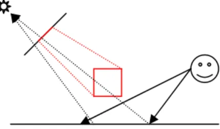
The shadow map algorithm [Williams 1978] is very straightforward, and in addition to its use in interactive applications, it is also extremely common in offline rendering for film production. The algorithm works by first rendering a depth map from the point of view of the light source. The depth map is an image where each pixel contains the distance from the rendered object to the light. When rendering the scene from an arbitrary viewpoint, the point under each pixel is transformed into the shadow map viewing space, and its depth is compared with the depth in the map. If the map’s depth is lower, the point is shadowed. This algorithm is illustrated in Figure 3-1. The main drawback to this technique is that the limited resolution of the shadow map image can produce jagged shadow edges, which detract from the realism of the image. A simple filtering technique called percentage closer filtering [Reeves et al. 1997] can be used to soften the appearance of the edges, and other, more involved techniques have also appeared recently in the graphics literature [Stamminger and Drettakis 2002, Sen et al. 2003].
Figure 3-1 : Shadow Mapping. A depth-image, taken from the light, is used to test for occlusion. The right point is in shadow, the left point is not
The shadow volume algorithm [Crow 1977, Heidman 1991] is more involved than shadow maps, but does not suffer from the jagged edge problem. This algorithm works by first locating the silhouette edges of a polygonal object, with respect to the light, and projecting those edges to infinity, creating a polyhedral volume. Any point which lies inside this volume is shadowed by the object. The technical report by Everett and Kilgard [2002] presents a number of techniques for robust implementation of shadow volumes. A key drawback to this technique is that in a graphics hardware implementation the volumes must be rasterized in order to determine whether each pixel is inside or outside the volume. This, together with the silhouette edge detection and geometry processing, typically makes the shadow volume technique much slower than using shadow maps, but the higher shadow quality often justifies the reduced rendering performance.
Both of the algorithms described above are limited to producing what graphics practitioners call “hard shadows”. This means that the shadows have sharp, geometric edges. Most real-life shadows are “soft”, meaning that there is a gradual transition between occluded and unoccluded regions. Soft shadows occur because most light sources are not simple point or directional sources, but are in fact extended, light emitting surfaces. The only physically correct way to render soft shadows is to compute the fractional visibility of the light, with respect to the shaded point. This is generally done by point-sampling its surface and computing the fraction of samples which are visible from the point of interest. In order to produce accurate shadows, a large number of sample points are required. There has been a great deal of recent work which has attempted to produce soft shadows from area light sources in interactive applications. We discuss a few of the most well-known methods here. For a more thorough review, we refer the reader to the recent survey paper [Hasenfratz et al. 2003].
The most intuitive technique for rendering soft shadows is to take a set of samples over the light emitting surface, and compute the illumination contributed by each sample point. When visibility is taken into account, this produces an accurate shadow image, but a large number of samples are typically needed, especially if the illumination produced by the light is not uniform over its surface. Various techniques such as importance sampling [Ward 1991] have been used to improve this process, but it can still be quite expensive. In our work we show how to efficiently compute the illumination from a point-sampled area light using programmable graphics hardware.
One recent technique approximates these shadows by extruding small, flat quadrilaterals, called “Smoothies” out of the silhouette edges of the object, rendering these into a texture from the light position, similar to a standard shadow map [Chan and Durand 2003]. Any surface that is occluded by the smoothie is assigned a visibility value that is computed based on the distance between the blocker and the light, and the distance between the receiver and the light. This technique, combined with standard shadow mapping for the umbra region, produces approximate soft shadows which are visually pleasing, but physically inaccurate. This technique is very similar to another approach called “Penumbra Mapping”, which was developed independently and published at the same time [Wyman et al. 2003].
Soft shadowing techniques based on shadow volumes have also been developed [Assarson et al. 2003]. These methods augment standard shadow volumes by using additional geometry (Penumbra wedges) to enclose the penumbra region. Fractional visibility is estimated for each pixel under the wedge by projecting the corresponding silhouette edge onto the light source and estimating fractional visibility. The visibility estimation is performed in a pixel shader, and the estimated visibility is accumulated into a screen-aligned texture which stores fractional visibility. The technique produces accurate shadows for rectangular or spherical lights, under most circumstances, but the per-pixel computation required can be expensive. Large area light sources amplify this problem, because they cause the creation of larger
wedges. The original work was targeted at interactive implementation on graphics hardware, but a variant of the technique has also been used to accelerate soft-shadow computation in a ray tracer [Laine et al 2005].
3.3 Global Illumination in Interactive Applications
Interactive implementations of ray tracing have been achieved for dynamic scenes [Parker et al. 1999, Wald et al. 2001], but a complex parallel computing architecture is usually required, and the algorithms used do not scale down to a single workstation with a commercial graphics accelerator. Specialized hardware architectures have been proposed for ray tracing, [Schmitteler et al. 2003, Woop et al. 2005] but these architectures do not yet achieve the same raw rendering performance as standard rasterization-based GPUs. Commodity GPUs have been used to accelerate the implementations of many of the traditional global illumination algorithms [Purcell et al. 2002, 2003, Carr et al. 2002, Cohen and Greenberg 1985, Coombe et al. 2004], but these implementations do not scale well to dynamic scenes, and even for static scenes they do not always achieve interactive frame rates even on modern GPUs.
An early attempt to adapt radiosity to dynamic scenes used a hierarchical structure of the patches of the scene, so that pairs of patches that were affected by a change to the scene could be detected and updated [Drettakis and Sillion 1997]. The main drawback of this work is that it is based on hierarchical radiosity, and thus requires a very fine subdivision of the surfaces in the scene in order to yield high-quality results.
Selective photon tracing [Dmitriev et al. 2002] is an improved photon mapping algorithm which is designed to support interactive rendering in scenes with moving objects. In this algorithm, a fixed number of photons are used to represent the indirect illumination, and are divided into a set of groups. One photon from each group, called a pilot photon, is shot during each frame in order to detect possible scene changes. When a pilot photon detects a scene change, all other photons in the group are re-shot and their contributions to the indirect illumination are adjusted.
A more recent work by Larsen and Christensen [2004] uses techniques similar to selective photon tracing, but performs the shading using graphics hardware. Photons are traced adaptively on the CPU in response to scene changes, and a final gathering approach based on hemi-cube radiosity [Cohen and Greenberg 1985] is used to compute a coarse texture map for indirect illumination, which is then applied to each surface. Caustics are also supported by using a screen-space density estimation technique over the set of caustic photons. The main limitation of this work is that the textures used for indirect illumination must be very small, because the textures are generated by rendering the scene once for each texel. In order to achieve high frame rates the authors had to use very coarse light maps and progressively update the illumination over several frames whenever it changed. This restriction to coarse textures limits the accuracy of the indirect illumination, but their method is able to efficiently render caustics.
Apart from the classical techniques, a variety of techniques have been developed specifically for handling global illumination effects in interactive applications. These techniques are too specialized to handle the general problem of accounting for all global illumination effects in dynamic scenes, but they typically provide an acceptable solution for specific cases.
Pre-computed radiance transfer [Sloan et al. 2001] is a technique which has attracted a great deal of attention in recent years. This technique supports interactive rendering of fixed objects under changing lighting conditions, and is able to capture a number of subtle effects such as interreflection and self-shadowing, which are difficult to compute using other methods. The main problems with this method are that it requires an expensive offline pre-processing step for each object, and dynamic changes to the object’s shape are difficult to support. We make use this method in our work, and will discuss it in more detail in Section 4.4.
A recent paper by researchers at the University of Central Florida [Nijasure et al. 2005] is probably one of the most effective examples of interactive indirect illumination on programmable graphics hardware. Their technique is to subdivide the volume of the scene into a coarse three dimensional grid, and compute a global illumination solution by repeatedly rendering images of the scene as viewed from each face of the grid. The images on the grid faces are then projected onto a spherical harmonic basis, and trilinear interpolation between grid points is used to compute the approximate indirect illumination for any point in the image. Because of the limited resolution of the cube grid, the algorithm does not correctly handle shadows in cases where indirect illumination is blocked by a nearby object, and it can also suffer from discontinuities in the illumination at grid boundaries.
3.4 Instant Radiosity
In this section, we introduce an indirect illumination technique called “Instant Radiosity” [Keller 1997], which our work will be heavily dependent on. This technique takes a different approach to indirect illumination, and despite its name, it is actually more closely related to monte-carlo ray tracing methods [Kajiya 1986]. Instead of subdividing the surfaces in the scene, instant radiosity begins by firing rays from the light into the scene, in the same fashion as photon mapping. The instant radiosity algorithm then treats each of the ray hit points as a point light source, which represents some of the indirect illumination in the scene. By rendering an image with shadows for each of these lights using direct illumination techniques; and accumulating the contribution of each image, a plausible approximation to indirect illumination can be computed. Keller’s original paper used graphics hardware and the shadow volume algorithm to render these individual light images, but did not achieve very high frame rates due to the large amount of per-pixel computation that is required.
Other researchers have picked up on the idea of representing indirect illumination as a set of point sources. Udeshi and Hansen [1999] present a modified version of this technique which estimates the amount of indirect light reflected by each scene polygon into the scene. The polygons are sorted according to the amount of light they reflect back to the scene, and the point lights are placed at the centroids of the first N polygons. The main problem with their work is that their implementation does not consider occlusion, that is, it does not take into account shadows caused by scene objects occluding these indirect lights. It is also very expensive to apply the polygon sorting technique to more than one bounce of indirect light, since this computation would be at least O(Nk) for N polygons and k bounces.
Wald et al. [2002] have also implemented global illumination algorithms using a modification of Instant Radiosity, but their technique uses a cluster based ray tracer [Wald et al. 2001] and is not designed to run on a single workstation with a GPU.
Another technique called reflective shadow maps [Dachsbacher and Stamminger, 2005] takes a creative approach to this problem. Reflective shadow maps are images rendered from the light’s point of view, in which each pixel acts as a point light source. When rendering an image with indirect illumination, the RSM is sampled several dozen times per pixel, and the contributions of the sampled pixels of the RSM are used to approximate the indirect illumination in the scene. The main limitation of this technique is that it does not consider occlusion. In addition, the technique assumes that pixels close to a point’s projection into the RSM will contribute more than pixels which are further away, and this assumption is not always accurate. Finally, the technique is limited to only a single bounce of indirect illumination. A recently published technique called Light Cuts [Walter et al. 2005] has been used to optimize instant radiosity in a ray tracing context by performing a clustering over sets of point lights. In this method, a hierarchical clustering is performed over all of the light samples in the scene, and a search through this tree is performed for each rendered pixel to locate the smallest set of clusters that meets a certain error bound. This method can reduce the number of light samples used from several thousand to several hundred, while still maintaining good image quality. The main drawbacks to this method are the fact that the initial set of lights must be very large (on the order of tens of thousands), and the fact that the clustering must be performed for each rendered pixel, which makes implementation on graphics hardware difficult.
4 Method
In this section we describe our techniques for rendering shadowed scenes using large numbers of point lights. We begin by discussing how point lights are distributed in our scenes. We describe our method for rendering omni-directional shadow maps in Section 4.2. In Sections 4.3 and 4.4, we discuss our approach to rendering the scene geometry. In Section 4.5, we describe how to progressively update the illumination computation in response to a change in the scene configuration.
4.1 Light Sample Generation
The first step in our technique is to generate a set of point lights to sample the illumination in the scene. Our method for doing this is a modification of Keller’s original instant radiosity technique [1997]. Our goal is to generate a set of oriented lights which represent the illumination transported by the surfaces in the scene. Each light sample will have a position, the normal to the surface on which it resides, and an intensity value.
For each light emitting surface in the scene, we generate two sets of point light samples. The first represents the direct illumination, and the second represents the indirect illumination. The relative sizes of these two sample sets can be adjusted according to the relative importance of direct and indirect illumination in the scene, and the total number of
lights can be increased if higher image quality is desired, or decreased to reduce rendering time and memory consumption.
The direct illumination samples are computed by selecting random positions on the surface of each emitter. The intensity of each direct illumination sample is equal to the power of the light source divided by the number of samples. Because we use a sampling of the area light source, our system implicitly computes accurate soft shadows for the direct illumination in the scene.
Our second set of lights represents the indirect illumination, and is computed by a random walk through the scene. A ray is fired from a random position on the light source in a random (cosine-weighted) direction, and a point sample is created on the first surface hit by the ray. The intensity of this sample is equal to the power of the light source scaled by the BRDF of the surface at the hit location. The process is repeated by recursively firing another random ray from the hit location until a user-specified bounce limit is reached, at which time a new ray is generated from the light source. The ray-shooting continues until the specified number of indirect light samples have been generated, at which point each sample’s intensity is divided by the total number of paths that were generated.
When distributing indirect illumination samples, we make one key assumption to simplify our algorithm. We assume that the effect of the moving objects on the distribution of indirect illumination is negligible. This assumption allows us to compute the set of sample points as a pre-process, using only the static geometry of the scene. This assumption will not be valid for scenes which contain very large movers, but it is a reasonable approximation for most scenes, since the majority of the indirect light is typically reflected by large stationary surfaces such as walls. This assumption also allows us to assume that the positions and orientations of the light samples in our scenes will not change.
4.2 Shadow Mapping
We use shadow maps, rather than shadow volumes, for our visibility computations, because we believe that they are inherently more efficient. Shadow volumes require a great deal of geometry processing for each light, since the silhouette edges of the objects must be extracted in order to generate the shadow geometry. More importantly, shadow volumes can also require a great deal of pixel processing, since the volumes tend to cover a large area of the screen. Clamping and culling techniques have been developed that will reduce the fillrate requirement [Lloyd et al. 2004], but these may not scale effectively to large numbers of lights. Using shadow maps also allows our graphics hardware implementation to compute the contribution from several lights in one rendering pass, which reduces both the memory bandwidth cost and GPU driver overhead. This is not possible with shadow volumes, since the volumes for each light must be rasterized in order to isolate the shadowed pixels.
4.2.1 Shadow Map Parameterization
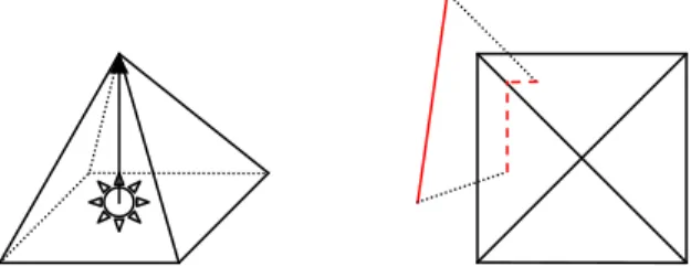
One of the most serious limitations of shadow maps is that they are difficult to use with point light sources. Standard shadow maps are implemented by rasterizing the scene geometry from the point of view of the light source in order to generate the map. If the field of view that is needed to cover the scene is very large, then standard shadow maps break down because graphics hardware cannot rasterize projections onto a full hemisphere (Figure 4-1). Because of this limitation, we must use a variant of shadow mapping which is able to represent the occlusion over the full hemisphere.
Figure 4-1 : A case where standard shadow maps break down. The shadow map must cover the entire hemisphere below the light to represent occlusion from both table legs. Graphics hardware
cannot rasterize projections onto a hemisphere.
Cube mapping is a technique for representing a function over the sphere by mapping a set of images onto the faces of a cube surrounding the sphere. In order to map a direction to a cube-map texel, the largest component of the direction vector is used to determine the appropriate face, and the remaining two components can be used to access the appropriate texel. All modern GPUs contain special-purpose hardware to accelerate this mapping operation. It is possible to implement omni-directional shadow maps by rendering the shadow map into a cube texture. There are, however, two problems with doing so. The first problem is that rendering into the six faces (five in our case) requires a large number of rendering passes. The main problem, however, is that cube maps make inefficient use of shadow map memory. In order to accurately represent shadows from distant occluders, the cube map resolution must be extremely high. In our case, this problem is amplified by the fact that the bottom face of the cube map will never be needed, (since our lights only illuminate over one half of the sphere) but there is no way to prevent the graphics hardware from allocating memory for it. Standard texture maps could, in principle, be used to simulate a cube map and avoid allocating the redundant memory, but this would be a very inefficient use of the API.
Figure 4-2 : Parabolic Shadow Mapping. Left: Projection of a line onto the shadow map. Lines in three dimensions can project to curves. Right: Accessing the map to test visibility for a particular
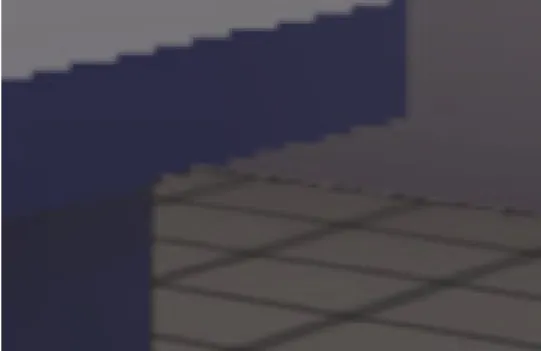
Paraboloic mapping [Brabec et al. 2002] is another technique which can be applied to functions over a hemisphere, and is more memory-efficient than cube mapping. In this technique, the scene is projected onto the surface of a paraboloid centered at the light position (Figure 4-2, left), and the resulting map is stored in a standard two-dimensional texture. When testing for visibility, the pixel shader computes the point on the paraboloid that reflects the direction of interest in the direction of the light’s normal, and uses this point to access the texture (Figure 4-2, right). Rendering into a paraboloid map requires only a single rendering pass with a relatively cheap vertex shader, and accessing the map during illumination computations can also be implemented very efficiently. However, because the projection of the scene onto the paraboloid is non-linear, it is not possible to generate an accurate shadow map without heavily tessellated geometry, because graphics hardware cannot accurately rasterize a non-linear projection. We have found this error to be a much more severe problem than the relevant literature indicates. The projection error is especially problematic if the shadow casting object is a large planar surface such as a wall, because the errors can result in thin slivers of light leaking through the bottom of the wall (see Figure 4-3). In this case, the artifacts cannot be eliminated without tessellating the walls to a size at which each triangle covers roughly one shadow map pixel. This level of tessellation is prohibitively expensive for our purposes.
Figure 4-3 : Light leaking artifacts due to inaccurate projection in a paraboloid map. The shadow on the far wall should extend to the floor. The walls are subdivided into a 25x25 vertex grid, but
the artifacts are still prominent. A tessellation level of 60x60 eliminates the artifact, but is too expensive for our purposes.
For our system, we use a technique which is combines the strengths of each of these two methods. We render our shadow maps by projecting the scene geometry onto the top four faces of an octahedron, and mapping the result onto a square as shown in Figure 4-4. Because the projections are linear, this mapping does not suffer from the artifacts that occur in parabolic mapping, and no tessellation of the scene geometry is required. This method requires up to four rendering passes for each shadow map, but this is still preferable to the five passes required for cube mapping, and the octahedral map is much more memory-efficient. Each rendering pass projects the blocker geometry onto one of the four faces of the octahedron, and user-defined clipping planes are used to constrain the rendering to the corresponding triangular slice of the render target. Computing the mapping between a point on the hemisphere and coordinates in the
map can be expensive in a pixel shader, since it involves a conditional projection onto one of four octahedron planes. Depending on the performance characteristics of the GPU, this cost could be reduced by pre-computing the texture coordinates corresponding to each direction on the hemisphere and storing the result in a cube map. As long as the cube map resolution is sufficiently high, no errors are introduced. This reduces the cost to one additional cube texture lookup for each shadow test. The memory cost of this cube map is negligible, since only one copy is needed.
Figure 4-4 : Octahedral Shadow Mapping. Left: An octahedron centered at a light source. Right: Projection of a line onto the shadow map. Note that the projection is linear over each face, but
discontinuous at the edges.
4.2.2 Shadow Map Rendering
Because of the large number of shadow maps that our system must deal with, we take great care to ensure that the shadow map rendering cost is as low as possible. We begin by taking the entire set of occluding objects and transforming the models into world space. We exclude from this set any surfaces which cannot block other surfaces (such as the outer walls of rooms). We do this transformation on the CPU, rather than on the GPU as it is normally done, because we cannot afford the overhead of specifying a different transformation matrix for each occluder in the shadow map. To do so would require changing vertex shader constants for each occluder and issuing a separate rendering command. This does not generally incur a great deal of overhead, but in our case, that small overhead is multiplied by a large constant factor. Performing the transformation on the CPU allows us to render all occluder geometry using no more than four rendering passes per shadow map.
After the transformation into world space, we perform a simple culling test for each shadow map face to determine if any of the four faces does not contain occluders. If this is the case, we are able to avoid rendering the projection onto this face, and in some scenes this produces a significant performance improvement.
Our shadow mapping vertex shader consists of two matrix multiplies. The first transforms the geometry into a light space coordinate system, (which is a rotation to align the Y axis with the light normal). The second projects the result onto the render target. User clipping planes are used during each pass to restrict the rendering to the triangular slice corresponding to the current octahedron face. Our pixel shader computes and stores the distance to the computed light-space position. This value is written out as the depth-value that is used for Z-testing.
4.3 Rendering Illuminated Scenes
Given our previously computed set of light samples, and assuming diffuse BRDFs for all surfaces (which are constant over the hemisphere), our goal at render time is to evaluate the following equation for each point x that is visible in the scene: ∈
=
Lights i i ii
n
x
G
p
x
V
L
x
A
x
L
(
)
(
)
(
,
)
(
,
,
)
Where:||
'
||
2)
'
'
)(
(
)
'
,
(
x
x
L
N
L
N
x
x
G
−
⋅
⋅
=
Li is the intensity of light i pi is the position of light i ni is the surface normal at point x
ni is the normal of the surface on which light i is located di is equal to pi –x (the direction from x to the light) V(x,y) is a visibility function between two points x and y A(x) is the reflectance of the surface at point x
There are several ways to optimize the above computation. The most obvious is to factor out the A(x) term, which is constant over the entire set of lights. We can implement this by rendering the diffuse albedo of the visible surfaces into a screen-aligned texture, and modulating the computed illumination by the albedo by using alpha blending. However, it is still expensive to evaluate the summation directly for each pixel. We employ a number of optimization techniques in order to reduce the cost of this computation. These techniques, taken together, can produce a significant speedup over a naïve implementation, as our results demonstrate.
The visibility function in the above equation is implemented by projecting each rendered point into the shadow map for each light. Because this must be done on a per-light, per-pixel basis, it can become prohibitively expensive. In order to reduce the cost of the visibility computation, we use a geometric algorithm to determine, for each object, which lights are potentially occluded, and which ones are definitely not. Because shadow map access is only required for partially occluded surfaces, we are able to avoid a great deal of redundant work by skipping the visibility computation for surfaces that can be shown to be free of occlusion. We use a hierarchical subdivision of the scene polygons in order to increase the effectiveness of this optimization.
Another avenue for optimization is to avoid repeated evaluation of the G function, since it is not view-dependent. This is accomplished by pre-computing the sum of LiG(x,n,i) into a texture map for each surface and ignoring visibility. At render-time, we take the interpolated illumination value from the texture map and subtract out the contributions of the occluded lights. This reduces our computational burden because it allows us to skip the illumination computation for the non-occluded lights.
We also simplify the computation by interpolating illumination from a low-resolution image, rather than re-computing it for each image pixel. This approximation is effective because illumination typically changes very slowly between pixels, especially when the surfaces in the scene are planar. The interpolation can produce unacceptable aliasing at object boundaries, but we can correct this aliasing by repeating the computation at full resolution for pixels that lie near an edge. Because interpolation is hundreds of times cheaper than re-computing illumination, we are able to drastically reduce the fillrate demand of our rendering system.
In addition to the algorithmic changes described above, we also structure our implementation to minimize the graphics API overhead that is entailed by repeated multi-pass rendering. When computing shadows, we process as many lights as possible in a single rendering pass, and we introduce an object clustering technique to minimize the required number of API calls.
4.3.1 Visibility Determination
As the number of lights in the scene grows, the large number of shadow map accesses per pixel quickly becomes a limiting factor. Because our rendering speed is so heavily tied to the pixel fillrate, we can obtain a performance boost by determining, for each element of the scene, which lights are potentially occluded and which lights are definitely not. This allows us to avoid shadow map accesses for unblocked lights on surfaces which obviously do not need them. For each rectangular surface patch in the scene, we perform this visibility determination by connecting each vertex of the patch to the light-source position, forming a skewed pyramid. Any object which does not intersect this pyramid cannot possibly cast a shadow on the patch. We can therefore separate the lights into unblocked, partially blocked, and fully blocked sets by testing each blocker object for intersection with the occlusion pyramid of each light. A light without any intersections is guaranteed not to be blocked over the surface of the patch. For complex models with a large number of polygons, we implement visibility determination at the object level, by widening the occlusion pyramid until it completely encloses the bounding sphere surrounding the object. The geometry of the occlusion pyramid is illustrated in Figure 4-5.
Figure 4-5 : Occlusion pyramids for planar surface patches (left) and complex objects (right).
Depending on the complexity of the blockers, we can choose to test each individual polygon against the pyramid, or to test a bounding volume such as a sphere. If the blocker contains a small number of polygons, it is advantageous to test the individual polygons, rather than the bounding volumes, because this yields more accurate visibility determination. In addition, it is possible to detect cases in which the entire object is occluded by a single large polygon. In such cases, the light can be ignored entirely when rendering the occluded object. For complex blockers, however, testing individual triangles against the pyramid can quickly become very expensive, and a bounding volume test can generally yield an adequate, conservative result. In our implementation, we make a distinction between simple surface patches like walls, which we test directly against the pyramid, and complex objects such as bunnies and teapots, for which we test only the bounding sphere against the pyramid.
Figure 4-6 : A 2D example illustrating hierarchical visibility determination. An object is recursively split two times, and the results of occlusion testing are shown for each node of the tree (F-full occlusion, P-partial occlusion, N-no occlusion). Leaves colored red do not require shadow
map access.
For very large surface patches such as walls, it is beneficial to subdivide the surface into smaller pieces. This allows shadow map accesses to be concentrated in regions of the surface where they are needed, which can reduce the rendering cost for the scene. We can make visibility determination more efficient by imposing a tree structure on the objects. For each light, we first perform the occlusion test for each of the parent patches, after first discarding any lights which are behind the patch. If a potential occluder is found for the parent patch, we recursively test the sub-patches until we reach a leaf, or until we find a sub-patch which is either fully blocked or unblocked. In this case, the
P
F P
occlusion testing is stopped and the result is propagated down the tree to the leaves. Our current implementation only performs this recursive subdivision on planar surfaces such as walls or floors, but it could in principle be applied to meshes as well by recursively splitting the mesh faces into clusters. Our subdivision strategy for patches is illustrated in Figure 4-6.
In our implementation, we found that subdividing large patches up to three times could produce performance improvements, but that excessive subdivision was generally not beneficial, since the overhead of adding additional rendering passes eventually outweighs the performance gained by not accessing redundant shadow maps. The level of subdivision for each surface in the scene should be set according to the degree of occlusion that is likely to occur on that surface. In our scenes, we used a fixed subdivision level for each surface, but we manually adjusted the subdivision according to the role of the surface in the scene. For example, we typically subdivided floors more heavily than ceilings. An adaptive subdivision could also be performed at run-time, using the number of occluded lights as a subdivision metric.
For static scenes, visibility determination for each light can be performed as a pre-processing step and stored. However, if the positions of objects change, then dynamic re-computation becomes necessary. We discuss how to handle moving objects in Section 4.5.1.
4.3.2 Light Mapping
For large, planar surfaces, such as walls, the illumination does not change rapidly over the surface (shadows notwithstanding). It is therefore possible to pre-compute the contributions of each light, to avoid having to compute light intensities at each pixel. We create a light map texture for each patch in our scene. This light map stores a sampling of the accumulated light intensity for the patch, for all lights which affect the patch and which are either unoccluded or partially occluded. We found that in order to prevent interpolation artifacts at the boundaries of sub-patches with differing illumination, it was necessary to maintain a separate light map for each sub-patch.
At run time, we first render the contents of these light maps into the frame buffer, using bilinear interpolation to smooth the illumination. The result of the first pass produces an illuminated image of the scene, without taking into account occlusion from partially blocked lights. We then make a second pass over the scene and use the shadow maps to subtract the contributions of occluded lights. The results of our visibility determination algorithm are used to optimize this process by applying a shadow map to a patch only if the light in question is partially occluded over the surface of that patch. We use this approach, rather than baking the shadows into the light maps, because it prevents our shadow
accuracy from being limited by the light map resolution, and because it reduces the need for light map updates when a shadow casting object moves.
Light mapping is based on the assumption that the surface has a diffuse BRDF. For non-diffuse BRDFs, this technique is not applicable, because the reflectance from the surface is view-dependent. If our surface BRDFs used a combination of diffuse and specular terms, as is often the case in practice, we could use the light maps to store the diffuse term, and compute the specular term dynamically, which would still allow us to avoid some of the computation. It may also be possible to store a compressed representation of the view-dependent reflected radiance function, using, for example, a spherical harmonic basis. However, this would require a great deal of storage, and dynamic updates would be difficult.
4.3.3 Lowres Pass
Even with visibility determination, the per-pixel computation that is required to render the image can still be very high. Fortunately, for large numbers of lights, the illumination changes between pixels on a flat surface are smooth enough that it is possible to compute a low-resolution sampling of the image and interpolate it into the high resolution image. This is similar in spirit to the irradiance caching technique which is commonly used to accelerate monte-carlo global illumination algorithms [Ward et al. 1988, Tabelleon and Lamorlette 2004]. This technique has been used before in interactive applications with a high fillrate demand [Dachsbacher and Stamminger 2005], and has proven to be a very effective means of boosting rendering speed.
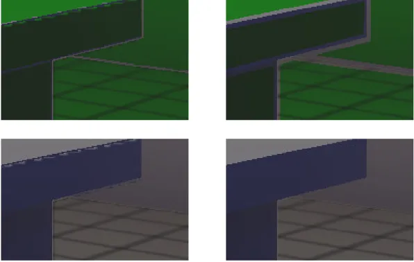
Figure 4-7 : Interpolation without edge detection. Although the illumination is smooth, the edges have an unacceptable jagged appearance.
Even though interpolation can produce a reasonable reconstruction of the illumination, it will also create jagged edges at object boundaries (Figure 4-7). This class of image artifacts is due to a phenomenon called aliasing, which is a common problem in computer graphics, and is caused by the limited resolution of a rendered image. To solve this problem, we render our images in two phases. We first render a low resolution image of the illumination, and then perform an edge detection operation to locate regions in which the surface orientation, and therefore, illumination,
changes rapidly. We will then perform a second rendering of the shadows at full resolution, which renders only to these boundary pixels.
We perform the edge detection by examining the texture maps which contain surface positions and normals for each pixel, and locating regions where the plane equations of the underlying surfaces change. When performing edge detection, it is necessary to mask out pixels in a wide region around the edges in order to prevent “color leaking” artifacts caused by the interpolation, as shown in Figure 4-8. We can implement this efficiently by stepping over a larger distance when examining neighboring pixels during edge detection. Although this simple approximation may problems at very thin discontinuities between surfaces, these cases are sufficiently rare in practice to justify its use. During the edge detection pass we set the depth value to zero at non-edge pixels, and one otherwise. This creates a depth mask, which we us