Publication quality tables in Stata:
a tutorial for the tabout program
Ian Watson [email protected]
Introduction
taboutis a Stata program for producing publication quality tables.1 It is more than just a means of exporting Stata results into spreadsheets, word processors, web browsers or compilers like LATEX. taboutis actually a complete table building program. This tutorial is intended to present a complete overview oftabout, with numerous examples of syntax and the kind of tables produced. You might like to flick ahead and skim these examples before reading the more detailed exposition which follows.
This tutorial has been around for a number of years but the current version makes use of colour and shading (to make it more readable) and also presents thetaboutcode in large blocks. Previously some of the preparatory Stata code, such as recoding variables, was only shown at the beginning of a set of tables. This meant that a user who just wanted to try out one particular table might have found that their results did not match the examples in this tutorial. At the risk of tedious repetition for those dedicated enough to begin at the beginning, the tutorial is now organised so that each example of code is ‘self contained’. The reader can now run any one of the examples in isolation and be guaranteed that the results should match what they see in this tutorial. All of the examples have sub-headings, so that readers can see at a glance what the particular example is illustrating. Finally, all of the examples are available in Stata do files which are installed whentaboutis installed from the SSC archives. The fileexamples_tab.docontains all the code for tab-delimited output (the default) and the fileexamples_tex.docontains the code for LATEX output.
I say a user’s results should match the examples in this tutorial, but I should add a caveat. I often get emails fromtaboutusers who don’t get exactly the same presentation quality which they see in this tutorial. This is due to the fact that this tutorial uses LATEX and makes use of the LATEX facilities built in to taboutto optimise LATEX code. These users are often exporting their results to MS Excel or MS Word and do not appreciate that LATEXis a totally distinct universe and requires learning a ‘new system’ for managing Stata output. I discuss LATEX more fully in the following pages, but would stress here thattabouthas many advantages for Stata users who are content to work in Excel or Word. In particular, it can automate many of the more tedious aspects of table production. Having dispensed with the housekeeping, it’s now time to explain whattaboutactually does. In essence,taboutallows a novice Stata user to produce multiple panels of cross-tabulations, and to lay out the data in a number of different ways. The output can be oneway or twoway tables of frequencies and/or percentages, as well as summary statistics (means medians etc). Standard errors and/or confidence intervals, based on Stata’ssvycommands, can also be included. Furthermore,
a number of statistics (chi2, Gamma, Cramer’s V, Kendall’s tau) can be placed at the bottom of each panel. Finally, formatting of cell contents is simple, and allows users to choose the number of decimal places, and to insert percentage symbols and currency symbols. Before looking more closely at some of the features available intabout, it is worth outlining briefly the design principles behind the program.
At a minimum,publication quality tables should be bothinformative andaesthetically pleas-ing. In his discussion of what makes for graphical excellence, Edward Tufte (2001) listed several important aspects of data presentation including the following:
1. present many numbers in a small space;
2. encourage the eye to compare different pieces of data.
While Tufte had graphs in mind, the same advice helps define what is meant by ‘informative’ when it comes to tables. In the case oftabout, multiple panels play this role. As will become evident later, repeating vertical panels allow for the succinct presentation of a considerable amount of data. Moreover, comparisons between populations and sub-populations within the one table are also easily achieved usingtabout.
Tufte’s book also canvassed aesthetics, though some critics might argue that his minimalist ap-proach to many of the classic statistical graphs has gone too far. Nevertheless, his core idea of max-imising the data component, and minmax-imising the decorative junk, makes for a lot of sense when it comes to table design. It coincides with the sentiments of Simon Fear, the author of the LATEX pack-age,booktabs(2003). With respect to the use of lines (called rules in LATEX), Fear advocated that
one should ‘never, ever use vertical rules’, and, more controversially, one should ‘never use double rules’. These principles—or at least the first one—are commonly followed in the tables presented in academic journals, and routinely violated in the business-type tables produced by spreadsheets.
Further refinements suggested by Fear (and implemented in hisbooktabspackage) include:
increasing the thickness of rules at the top and bottom of tables compared with the lines used for the mid-rules; and using a small but discernible amount of additional spacing above and below rules. Anyone who has tried to implement these principles inside a word processor knows how tedious this task is, making LATEX the obvious choice for achieving aesthetic goals such as these. In the case of tabout, the aesthetics largely come through exporting the output as a LATEX docu-ment and making use of a number of taboutoptions. These include variable rule thicknesses and spacings, rules which span a set number of columns, and the rotation of value labels in the table headers to achieve an economical layout which avoids the ugliness of hyphenation. An additional advantage in using LATEX withtaboutis the ease with which it allows for the batch production of tables, particularly large numbers of routine tables (as often occurs in an appendix).
For Stata users contemplating leaving their word processors behind and trying out LATEX, there are a large number of tutorials and other free materials available on the web. Two books which have been a staple in my library for many years are Goossens, Mittelbach and Samarin (1994) and Kopka and Daly (1999), both of which have been recently updated.
Despite my bias towards LATEX,taboutalso provides many advantages to those Stata users who import their descriptive tables into spreadsheets or word processors, or require html output. As will be evident below, these users can also gain great efficiencies in usingtabout, since very little further processing of the cell entries is required once the appropriate options have been turned on intabout.
Principles of user-friendliness underlie both the design and the syntax oftabout. Whiletabout aims to offer considerable customisation and flexibility to the end user, it tries to do this without becoming overly complex. It stays close to Stata principles, and also implements a number of con-sistent requirements in its syntax. There is a preference for single terms as options, either as a switch
(simply turning onsvy, for example to achieve survey results) or as a switch with a single value (such
as thelayoutoption).taboutavoids options within options, with the consequent need for
numer-ous balanced parentheses. Instead, using two or three separate switches (where needed), each with a single value, is the preferred approach. Thenoption, for example, which provides sample counts
in a table has five siblings: annpos(the position), annlab(the label), annwt(the weight), annnoc
to suppress the display of commas and annoffsetto control placement of n counts. taboutalso
allows for the ‘incomplete’ entry of values, and makes up the additional values by repeating the last value entered (for example, with formats or labels). Finally,taboutalso tries to capture most syntax errors at the outset and to provide a simple explanation. To facilitate this, a table outlining the allowable features of taboutis presented to users when they make syntax errors. (This table is presented later in this tutorial.)
Overview
What kinds of tables does taboutproduce? Using a simple terminology, you can producebasic
tables andsummarytables. The first are twoway and oneway tables of frequencies and percentages. Essentially, all of the output from Stata’stabulateis available in a basic table. You can also produce
basic tables with standard errors and confidence intervals, reflecting most of the output from Stata’s
svy:tabcommands. As forsummarytables, these are twoway or oneway tables of summary
stat-istics derived from Stata’ssummarizecommand but laid out in a much more aesthetically pleasing
fashion. In many respects, these tables mimic most of the output from Stata’stabstatandtable
commands. Finally, you can also have summary tables with standard errors and confidence inter-vals, though this is restricted to mean values. These tables make use of Stata’ssvy:meancommand.2
With a large dataset, the survey option intaboutcan be quite slow. This is partly because the sur-vey commands run slower in Stata 9 than they did in previous releases, and partly becausetabout needs to run the survey commands twice to retrieve column and row totals. The latest version of taboutnow includes the ‘dot counter’ view, which indicates to the user that something is actually happening (however, slowly).
With a basic table, the cells in a table can be any one or all of the following: frequencies, cell percentages, column percentages, row percentages, cumulative percentages. With summary tables the list is quite extensive: N mean var sd skewness kurtosis sum uwsum min max count median iqr r9010 r9050 r7525 r1050 p1 p5 p10 p25 p50 p75 p90 p95 p99.3
There is considerable flexibility in the layout of the tables. All tables can be produced using mul-tiple ‘vertical’ panels if desired. A command liketabout occupation industry southwill
pro-duce two vertical panels (variables occupation and industry) cross-tabulated against a ‘horizontal’ variable, south. The cell contents can be laid out in columns or rows (for example, frequencies and column percentages alternating, as in: No. % No. % No. %). They can also be laid out in column block(abbreviated to cb) orrow block(abbreviated to rb) mode. For example, frequencies and column percentages can be in contiguous blocks, as in: No. No. No. % % %).
As well as the contents of the cells, additional information can be placed in the table. The most notable of these inclusions are sample counts (or population estimates),⁴ which can be placed in the far right column, along the bottom of the table or alongside the value labels in the first column. A range of statistics can also be included at the bottom of the table. These consist of: Pearson 2 If aniforincondition is specified with any of thesvyoptions,taboutmakes use of thesubpopulationoption, as
recommended in the Stata manual.
3 The uwsum is not mainstream Stata. It stands for ‘unweighted sum’ and is a useful statistic in tables where you to present weighted data, but would like one (or more) columns to contain an unweighted sum of a variable. For example, ‘uwsum subpop’ can be used to create an ‘n’ count in the middle of a table of means.
⁴ The main difference between these two is that the latter are weighted counts, achieved throughtabout’snwtoption.
Note that you need to use thepopoption when you are also using survey data (with thesvyoption) in order to achieve
chi2, gamma, Cramer’s V, Kendall’s tau and the likelihood-ratio chi2. Finally, you can also include additional information at the bottom of the table, such as the source of the data, the population or various notes. Headings and sub-headings for tables can also be placed at the top of the table.
The table below summarises these categories of tables, the kinds of contents allowed and the available layouts. (As mentioned earlier, if you make an error when typing the syntax of tabout, the following table is displayed on your screen, alongside a hint as to the nature of your error.)
Type of table Allowable cell contents Available layout
Basic freq cell row col cum col row cb rb
any number of above, in any order for example: cells(freq col)
Basic with SE or CI freq cell row col se ci lb ub col row cb rb
only one of:freq cell row col (turn onsvyoption) (must come first in the cell)
and any number of:se ci lb ub
for example: cells(col se lb ub)
Summary any number of:N mean var sd skewness no options (fixed) -as a oneway table kurtosis sum uwsum min max count
median iqr r9010 r9050 r7525 r1050 (turn onsumoption; p1 p5 p10 p25 p50 p75 p90 p95 p99 also may need to turn with each followed by variable name
ononewayoption) for example: cells(min wage mean age)
Summary only one of:N mean var sd skewness no options (fixed)
-as a twoway table kurtosis sum uwsum min max count median iqr r9010 r9050 r7525 r1050 (turn onsumoption) p1 p5 p10 p25 p50 p75 p90 p95 p99
followed by one variable name for example: cells(sum income)
Summary with SE or CI meanfollowed by one variable name col row cb rb (turn onsumoption and any number of:se ci lb ub
andsvyoption) for example: cells(mean weight se ci)
Syntax
tabout varlist [weight ][if ][in ] using [, replace append cells(contents) format(string) clab(string) layout(layouts) oneway sum stats(statstypes)
VARIOUS ‘N’ OPTIONS:
npos(positions) nlab(string) nwt(string) nnoc noffset(textrm string) VARIOUS SVY OPTIONS:
svy sebnone cibnone cisep(string) ci2col percent level(#) pop USER CUSTOMISATION OF LABELS:
total(string) ptotal(totaltype) h1(string) h2(string) h3(string) STYLE OPTIONS, MOSTLY FOR LATEX OUTPUT:
style(styles) lines(linetypes) font(fontstyles) bt rotate(#) cl1(#-#) cl2(#-#) cltr1(string) cltr2(string)
OPTIONS RELATED TO EXTERNAL FILES:
body topf(string) botf(string) topstr(string) botstr(string) psymbol(string) delim(string) MISCELLANEOUS OPTIONS: dpcomma money(string) mi sort chkwtnone debug noborder show(showtypes) wide(#) ]
wherevarlistis a list of vertical (row) variables, followed by the horizontal (column) variable last. if theonewayoption is specified, then all the variables are regarded as vertical.
wherecontentsconsist of:freq cell row col cumfor basic tables andN mean var sd skewness kurtosis sum uwsum min max count median iqr r9010 r9050 r7525 r1050 p1 p5 p10 p25 p50 p75 p90 p95 p99for summary tables. The default isfreq. When thesvyoption is used, you
can also specifyse ci lb ub.
wherelayoutsconsist of:col row cblock rblock. The default iscol.
wherepositionsconsist of:col row both lab tufte. The default iscol.
wherestatstypesconsist of: chi2 gamma V taub lrchi2, though onlychi2is available forsvy
tables.
wheretotaltypesconsist of:none single all. The default isall.
wherestylesconsist of:tab tex htm csv semi. The default istab. csvuses commas whilesemi
uses semi-colons. texis used for producing output suitable for LATEX documents.
wherelinesconsist of:single double none. The default issingle.
wherefontstyleconsist of:bold italic. The default is plain formatting.
whereshowtypesconsist of:none all output. The default isoutput.
fweights aweights iweightsandpweightsare allowed withtabout, depending on the underlying
command; see [U]14.1.6 weightand individual entries fortabulateandsummarize. For tables
of summary statistics,iweights are not allowed, becausetaboutuses thedetailoption in Stata’s summarizecommand (which does not allowiweights. Note that thesvyoption requires that the
data be alreadysvysetand an error message reminds you of this if you forget. The weight set by svysetwill override any other weightcommand you entertaboutif you have specified thesvy
option.
Options
using is required, and indicates the filename for the output. Some applications (particularly MS
Excel) ‘lock’ files when they’re open.taboutcannot write to these files and consequently issues an error message, suggesting that you check to see if the file is already open in another application. There is now a discussion of this problem in the ‘Tips and Tricks’ section below.
replaceandappendare file options, and determine whether the current output will overwrite an
existing file, or be appended to the end of that file. If you omitappendorreplace,tabout
issues a warning if the file already exists.
cells determines the contents of table cells. As the table on the previous page showed, you
can enter any one or more offreq cell row col cumin a basic table. They can be in
any order. When you choose thesvyoption, you can only have one of these choices, and
it must come first. The additional choices which are then available are: se ci lb ub.
For summary tables, you can have any of thecontentslisted earlier. If you are creating
a twoway table, only one summary statistic may go in a cell (eg. median wage); if it’s a
oneway table, any number of statistics (followed by a variable name) may go in the cell (eg. median wage mean age iqr weight). When you choose thesvyoption with
summary tables, onlymeanis allowed (eg.mean wage se ci.)
format indicates the number of decimal points. Unlike mainstream Stata, this option only
requires a number. Do not enter ‘%’ or ‘f ’ symbols. You can however, entercfor comma,p
for percentage, andmfor money (currency) and you can use themoneyoption (see below)
to specify the currency. For example, you might enterf(0c 1p 1p 2)to produce: 1,291
9.2% 10.3% 23.93. The entries should be in the same order as thecellsorder, that is, if freqcomes first, then0cshould come first if you want 0 decimal points (with commas)
as the format for frequencies. You do not have to type in the same number of format entries as there are cell entries. If you include more,taboutignores them; if you include less, the lastformatentry is repeated for the remaining cell entries. You can change the
decimal point and thousand separators to the style favoured in some European countries (, for decimal points . for thousands) using thedpcommaoption (see below).
clab determines the column headings for the third row of the table, that is, the headings just
above the data. By default,taboutplaces the ‘horizontal’ variable’s name in the first row, its value labels in the second row, and an abbreviation for the cell contents (eg. No. Row % etc) in the third row. You can over-ride all of these defaults using theh1 h2andh3
options (see below). Most of the time, however, it will only be the third row which you need to change, so theclaboption makes this easy for you. Just enter the column titles
as you want them to display, without quote marks or other symbols.However, you must include underscores between words if there are spaces in the column title, for example
clab(No. Row_% Col_%). You do not have to type in the same number of clabentries
as there are cell entries. If you include more,taboutignores them; if you include less, the lastclabentry is repeated for the remaining cell entries. For example if your cell entry
wasfreq col row cumyou could just enterclab(No. %)and all but the first column of
data would have % symbols at the top.
layout determines how the columns will be laid out. They can be in alternating columns (No.
% No. % No. %) and alternating rows (No. on the first row, % on the next two, then back to No. and so on). They can be in column blocks, or in row blocks, where the data is kept contiguous, for example: No. No. No. % % %. The exception to this is summary tables where the layout is fixed and you have no choice. (However, an
exception to this is thesvyoption, which can be laid out using all of these options. See
the earlier table for clarification.)
oneway tellstaboutthat the list of variables are all ‘vertical’. Normally,taboutassumes that the
last variable in the list is the ‘horizontal’ variable, to be used in a twoway cross-tabulation. To override this default behaviour, specifyoneway. If there is only one variable in the
variable list,taboutassumes it is a oneway table, so you don’t need to issue theoneway
option in this case.
sum tellstaboutthat the table is to be a summary table. Normally,taboutassumes that the table
will be a basic table and checks to see if thecellscontents have the correct entries (freq row coletc). By tellingtaboutthat the table is a summary table, this checking process
includes checks for the various summary statistics and the variables in the data set. The
sumoption is essential if you wish to produce a summary table.
stats allows you to include additional information based on the various statistics available in tabulate. Note that, unliketabulate,taboutrequires that you enter the full term (and
not an abbreviation) and will only allowonestatistic in a table. You must enterchi2, not
justchi.
npos determines where the ‘n’ information will be place. The various ‘n’ options (npos nlab nwt nnoc) provide sample counts for the table. You need only enter one of these options
for the ‘n’ to be included. For the options you have not entered,taboutplaces make use of the default values.A cautionary note: if you selectnpos(row)and are using multiple
panels, the n counts you see at the bottom of the table reflect only those observations included in the bottom panel. They may not be accurate n counts for panels higher in the table, depending on whether there are missing observations in the bottom panel’s vertical variable.
lab determines the label for the ‘n’ counts. The default forcolandrowpositions is a simple
uppercase N; for thelabposition it is(n=#)where # stands for number; and for thetufte
position it is(#%). You can change all of these except thetufteposition (which is fixed),
and if you wish to alter thelabposition, use the # symbol to indicate where the number
should go. For example,npos(lab) nlab(Sample count=#). Thenpos(tufte)option
provides a convenient way of displaying a percentage breakdown, rather than a count, for the main ‘vertical’ variables. The name comes from the approach adopted by Edward Tufte in his construction of a ‘supertable’, which he designed for theNew York Timesin 1980 (2001, p. 179).
nwt indicates that the ‘n’ count be weighted by this variable. This can be useful for producing
population estimates in a table, rather than just sample counts. Note thattaboutalways uses Stata’siweightoption for this weighting.
nnoc stands for n-no-comma and turns off the comma in the ‘n’ count. Becausetaboutdoes
not provide aformatoption for ‘n’ counts (decimal points don’t really make sense here),
the default behaviour is to include commas. Thennocoption over-rides this default
be-haviour.
noffset stands for n offset and determines where the n counts should be placed. The default
is 1, which means the n counts will be in the first data column and/or the first data row in a table. Settingnoff(2)for example, allows you to shift the n counts further along (or
down) in the table, into either the second data column or the second data row. If you are using block layouts (layout(cb)orlayout(rb)), thenoffsetoption applies to blocks
svy tellstaboutthat thecellcontents include survey output, and so the checking procedure
(mentioned earlier) looks for things likese,ciand so forth. You must turn onsvyis you
wish to include survey output in your table.
sebnone stands for se-brackets-none and tellstaboutto suppress the parentheses which
nor-mally surround the standard errors.
cibnone stands for ci-brackets-none and tells taboutto suppress the square brackets which
normally surround the confidence intervals.
cisep stands for ci-separator and tellstaboutto replace the default (which is a comma) by
whatever the user enters (for example, a dash).
ci2col stands for ci-in-two-columns and tellstaboutto place thelbandubestimates in two
columns (as it normally does), and to place a ‘[’ and a ‘,’ in the first column, and a ‘]’ in the second column. This can be useful for layout in a word processor, because the first column can be right aligned (to the comma) and the second column can be left aligned, and it appears that you have a single column for your ci, which is neatly aligned according to the commas. Note that if you selectciin thecells,taboutnormally places both the
lower bound and the upper bound in a single cell and includes brackets and separator. Theci2coldoes not apply in this case. For it to work, you need to specify the upper and
lower bound options, for example:cell(freq lb ub) ci2col.
percent tellstaboutthat thesvyoutput should be shown as percentages, not proportions. This
follows the default behaviour ofsvy:tab.
level specifies the level for thesvyestimates. The default is 95%.
pop specifies that a weighted population estimate should be provided for the n in the table, rather
than the sample size. This option makes use of the weight specified by thenwtoption.
This makes thesvyoption work the same as thenwtoption with non-survey tables. To
get weighted estimates, rather than sample counts, you need to specify bothnwtandpop.
The weight specified innwtmay be the same as that used when yousvysetyour data, or
it may be different. You may want the estimates in the table weighted by ‘effective sample size’ weights, while you want your n row or column to show population estimates based on ‘expansion’ weights.
total tellstaboutwhat labels to use for totals. The ‘vertical’ total comes first, the ‘horizontal’
second. The default labels for these variables are ‘Total’. If there are spaces in either of the labels which you wish to enter, use underscores. For example,total(All_persons Total).
ptotal tellstabouthow to treat the totals for each panel, when you have multiple panels in a
table. The default behaviour is to show all totals, but this can sometimes be repetitive, so you can specifyptotal(single)to have a single total row shown at the bottom of the
table. You can also turn off all totals withptotal(none).
h1through toh3over-ride the default headings for a table. If you choose to use these, there are a
couple of requirements. If you have selected eithertexorhtmas your output style, you
are responsible for all the various code needed. taboutdoes not makeanyadjustments to what you enter, it just outputs it as it finds it. If you have chosentab,csvorsemias
your output style, you must enter a delimiter to indicate where the columns are in your heading. Unlike the usualtaboutpractice, you do not need to worry about spaces in your titles (no need for underscores!) because this column delimiter takes care of things. However, the number of delimiters must match the number of columns in the table or the headings may be out of alignment. You might enter: h2( | Very good | Good | Bad | Very bad | Total | N)and the first column heading would be empty, and the
remaining columns would have the appropriate labels. Note that thenpos(col)option
usually places thenlabon theh2line so you may need to include this yourself in yourh2
label, as in the example just given. To suppress the display of any of these headings, enter ‘nil’ into the appropriate option (for example,h3(nil)). While it is rare to write headings
longer than 256 characters, problems have been reported when this limit is exceeded.
style The default isstyle(tab), which is useful for importing into spreadsheets or word
pro-cessors. Note that the first row always has the correct number of tabs, even when a single title is involved. This helps other applications parse the table correctly. Note also that the repetition of labels in headings can be easily dealt with by using a ‘merge cells’ command in your spreadsheet or word processor. Thestyle(csv)andstyle(semi) options are
useful for importing into spreadsheets (like MS Excel) because the file generally opens immediately as a spreadsheet. Note, however, that some spreadsheets ignore trailing 0s, so this may muck up your neat formatting. To avoid this, export the table fromtaboutas
style(tab)and use the wizard in your spreadsheet to indicate that all columns are ‘text’
rather than ‘general’.
lines indicates how much space (forstyle(tab),style(csv)andstyle(semi)) or how many
lines (forstyle(tex)) should separate tables between panels. The default issingle. font only applies to style(tex)andstyle(htm)and provides bold and italic fonts for the
‘vertical’ variable names and the ‘horizontal’ variable names and value labels. The totals are also given this font. You can also use theh1toh3options to manually set up fonts for
your titles.
bt only applies to users of LATEX, and requires that you have thebooktabspackage installed.
This allows the use of the toprule, midrule and bottomrule commands, rather than the usual hline command. It produces more pleasing output.
rotate only applies to users of LATEX, and can be used to rotate the ‘horizontal’ variable’s labels
through whatever angle is entered in this option. For example, rotate(60)produces
quite a pleasing effect. You will also need to include the following LATEX code (courtesy ofgoossens1997) in your document’s preamble:
LaTeX code for rotation of table headings
\newcommand{\rot}[2]{\rule{1em}{0pt}% \makebox[0cm][c]{\rotatebox{#1}{\ #2}}}
cl1andcl2only apply to users of LATEX, and also requires that you use the booktabs package in
your LATEX document. These options can be used to place horizontal lines which span several columns (called, column lines, hence cl) and which are placed between the first and second heading rows, and between the second and third heading rows (hence two sets). You enter the column numbers which you wish to span, separated with a dash. For example, to place a line under the ‘horizontal’ variable’s name, you might enter:cl1(2-6)
in a table with six columns. If you are entering lines spanning blocks of columns (2-4 5-7), you might need to fine tune the gap between them usingcltr1andcltr2. By default,
whenever you specify either of thecloptions,taboutplaces a small gap (0.75em) between
adjacent lines.
cltr1andcltr2stand for column-line-trim, and allow you to specify an amount of trim to be
applied to the left side of thecl1orcl2lines which you have entered. You can specify
the amount in whatever acceptable tex measurement you like. For example:cl2(2-3 4-5 6-7) cltr2(1.5em). As just noted, the default amount is 0.75em.
body is used to insert some basic html or LATEX code above and below the table. This allows you
topfandbotfallow you to insert code stored in files whichtaboutcan insert above and below the
tables. These are particularly useful for html and LATEX users, and allow you to control the layout of the tables more precisely. All users will find them useful as a way of insert-ing additional information above and below the table, such as notes, populations, data sources (for the bottom of the table) and titles (for the top of the table).
topstrandbotstr contain text which you can pass to the topfandbotf files. This text will
be inserted into the files where ever the placeholder (default #) has been placed. Note that each placeholder must be on a separate line in these files. The strings designated in thetopstrandbotstrmust be separated with the pipe delimiter (or other user-chosen
delimiter) if there is more than one block of text being passed.
psymbol stands for placeholder-symbol and can be any symbol the user chooses. The default
is # and it provides a ‘placeholder’ in the stored files (thetopfandbotf) whichtabout
places above and below the tables.
delimit can be any symbol the user chooses. The default is the pipe delimiter as shown in
the earlier example. It is used to specify columns within theh1toh3options, and for
separating the contents of thetopstrandbotstroptions.
dpcomma specifies thattaboutshould use commas for decimal points and periods (full-stops)
for thousand separators. This style is common in many European countries. This op-tion affects the presentaop-tion of both the tabular output and the statistics when these are requested (such as chi2).
money indicates the currency to be used if you have chosen the money format. For example, format(2m) money(£). You can enter any symbol that your keyboard allows. For LaTeX
users, you can enter any text which LaTeX accepts, though you may need to include quotes.
mi specifies thattaboutshould display missing values. This works the same as themioption in
Stata’stabulatecommand.
sort specifies thattaboutshould display values in oneway tables in descending order of
fre-quency. This works the same as thesortoption in Stata’stabulate onewaycommand.
Note that if you issue this for a twoway table, you will receive an error message. This is becausetaboutis built on top of tabulateand the latter does not support sorting in
twoway tables.
chkwtnone preventstaboutfrom checking the legality of your weights. Statacommands will
not allow you to use non-integer frequency weights andtaboutnormally checks for this. You can over-ride this behaviour with the tt chkwtnone option. Note that this option does not stopStataitself from refusing to use non-integer frequency weights.
debug shows you most of the underlying Stata commands (though not for summary tables)
from which the tables are built. This can be useful for confirming your results.
noborder only applies to html output, and determines whether the table and cells should be
surrounded by borders. This only applies when thebodyoption is turned on.
show determines what will be seen on the screen. Theshow(all)option displays the final table
output as well as the Mata string matrices which are used to build this final output. The contents of these matrices may not exactly match the final output, in terms of formatting and labelling. Theshow(none)option suppresses all output except for the name of the
file to which the table has been exported. The default option is to show the output which has been sent to a file. It may look messy on the screen, but open it in the appropriate application to check it first before panicking.
wide is used in conjunction with show(all)and specifies the width of the columns in the
Mata matrices. The default is 10 spaces. Note that even if you reduce this to a very small number,taboutwill always increase the width of the columns to accommodate the widest cell entry in the data.
Some examples
If you want to dive straight into the examples, please read this paragraph first! The code which accompanies all the examples below has a linerep ///somewhere in the middle. If you are a
user who only wants delimited text files—that is, you’re not a LATEX user—don’t use the code below this line. The code fromstyle(tex)onward is for LATEX users. If you’re uncertain, just look at the
ancillary files fortabout:examples_tab.dowhich contains all the code for tab-delimited output (the default) and the fileexamples_tex.dowhich contains all the code for LATEX output.
In the following examples I present some tables based on several of Stata’s shipped datasets, though they mainly draw on thenlsw88.dtadataset. This is a handy dataset for illustration because it has so many categorical variables (apologies to those with a more medical inclination to their stats.). All these shipped datasets can be loaded with thesysuse command. In the case of the nlsw88.dta, a weight variable was also constructed (using a random number multiplied tenfold) so as to demonstrate thesvyoption.
A note on the examples and typefaces. In the discussion up to now, and in the syntax and options sections above, this tutorial has followed the Stata convention and shown the command options in the same way they are presented in the Stata manual.⁵ However, for clarity and readab-ility, from now on the typeface departs from the Stata convention in a couple of ways. References to other Stata commands are in the normal roman font, but areboldedand references totabout’s own options are in asans serif blue font(Urbana SemiBold for those interested). This makes it easy to discern what thetaboutoptions are, which should make it simpler when it comes to checking the options section when you want to read more about a particular feature.
A brief note on abbreviations is also worth making. In the examples which follow I use the full wording in the first part of the example code so that users will know what is going on. This even applies to variable names, for example, using ‘occupation’ rather than the much shorter, ‘occ’. However, as the examples continue, I begin to use the abbreviations. If you’re not sure about this, check the syntax diagram where the underlining indicates the abbreviated version of an option.
While the actualtaboutsyntax (the code) in the following examples does follow the Stata con-vention of using a fixed typewriter font, the background is shown as a grey shading. This makes it easier for the casual reader to see what is going on. In addition all of these blocks of syntax are labelled so that they directly relate to the example output. The output itself is shown in a blue sans serif font. Cutting and pasting from these blocks of syntax into Stata should produce the same res-ults as you see in this tutorial. A word of warning though. If you cut and paste from a PDF file (like this tutorial) quotation marks may not copy correctly and you may come to grief with macros, since Stata requires you to distinguish between the back quote and the normal quote. This warning mainly applies to the Tips and Tricks section, where macros are used a fair bit.
For LATEX users, copying and pasting the code should produce identical results to those shown in this tutorial if you run the whole block. The only change you will need to make is to replace
table1.txtwithtable1.texetc. The surrounding LATEX table commands are not shown, but are found in the top file and bottom file text shown after the examples section of this tutorial. Once you create these files and place them in your own working directory, you should not need to worry about them again.
⁵ The only exception to this has been that the wordtabouthas been presented in bold roman font throughout this tutorial, rather than the fixed typewriter font normally used for Stata commands.
For those wanting tab delimited output, stop at the line ‘replace’ and ignore the remaining LA TEX-specific code. In order to get the nice layouts and formats you see here, you’ll need to fiddle with your spreadsheet or word processing format controls. Finally, the replace option is redundant if you are only running these blocks of code once (so just ignore the error message).
If you prefer not to cut and paste from this tutorial, there are ancillary files which should install when you first install taboutfrom the SSC archives. These are example do-files which you can directly run in Stata. These files do not contain abbreviations and show the full name of alltabout options. There are two files, which are just different versions of the same set of examples:
1. example_tex.do: which has all the code shown in these examples (that is, the additional LATEX options) and which sends the output to tex files; and
2. example_tab.do: which has the first part of the code (up to the replace line), and which sends output to tab-delimited text files.
There are also two other ancillary filles—top.texandbot.tex—which are used extensively in the LATEX examples. There is a discussion of these files on page 33 below. You can either create your own version of these files, or use the versions included here.
While it might appear from the following examples that the top file and bottom file options are only useful for LATEX and html users, this is not the case. All of these examples show the source of the data as a note at the bottom of the table, and this device may be useful to all users. Indeed, en-capsulating titles, notes, sources, populations, weighting information, and so forth within the code which produces a table is a very good practice, and is particularly useful for the batch production of tables, where copying such information bit-by-bit is error prone.
If you are a tab-delimited or csv user, have a look at the code for the contents of these files at the end of this tutorial and you will see how you can also make use of top files and bottom files for including extra information with your tables. Just ignore the LATEX verbiage and focus on how the # symbol is used. This is the key to passing variable information, such as the population description for a table, to a fixed set of phrases which are the same in all tables. For example, the phrases “Notes: Estimates weighted. Source: mysurvey.” might be repeated for all your table, while phrases like “Population: All males over 21 year of ages” might vary between different tables. By using a simple bottom file (with the contents of the fixed phrases) and then adding the # symbol at the end, you could then pass different ‘arguments’ (the phrases which vary) to the information which will print at the bottom of your table.⁶
⁶ Note that while the examples in this tutorial just show the use of one argument being passed to a file, you can use multiple arguments. Just add as many # symbols as you need. However, make sure each # symbol is on a new line in your top and bottom files. Inside yourtaboutsyntax, just use the pipe delimiter (or your defined symbol) to separate all the arguments.
Basic tables
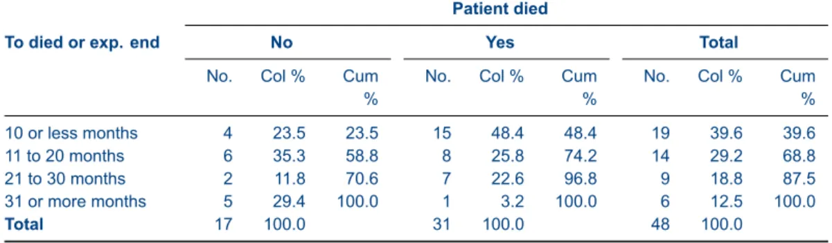
Whiletaboutis based closely ontabulate, it goes a bit beyond it. Not only can you specify the
cellscontents in any order you please—and they will display in that order—but you can also use cumulative percentages inside twoway tables. The following table illustrates this possibility. Table 1: Example of simple cross tabulation
Patient died
To died or exp. end No Yes Total
No. Col % Cum %
No. Col % Cum %
No. Col % Cum % 10 or less months 4 23.5 23.5 15 48.4 48.4 19 39.6 39.6 11 to 20 months 6 35.3 58.8 8 25.8 74.2 14 29.2 68.8 21 to 30 months 2 11.8 70.6 7 22.6 96.8 9 18.8 87.5 31 or more months 5 29.4 100.0 1 3.2 100.0 6 12.5 100.0 Total 17 100.0 31 100.0 48 100.0 Source:cancer.dta
Stata code for Table 1
sysuse cancer, clear
la var died ”Patient died”
la def ny 0 ”No” 1 ”Yes”, modify la val died ny
recode studytime (min/10 = 1 ”10 or less months”) /// (11/20 = 2 ”11 to 20 months”) ///
(21/30 = 3 ”21 to 30 months”) /// (31/max = 4 ”31 or more months”) /// , gen(stime)
la var stime ”To died or exp. end”
tabout stime died using table1.txt, ///
cells(freq col cum) format(0 1) clab(No. Col_% Cum_%) /// replace ///
style(tex) bt cl1(2-10) cl2(2-4 5-7 8-10) font(bold) /// topf(top.tex) botf(bot.tex) topstr(14cm) botstr(cancer.dta)
After some recoding to improve presentation, this syntax illustrates a number of features of tabout. Theformatoption only needs two entries, and the third item in the cell contents (the cu-mulative percentage) is automatically assigned the second format. The underscores are used in the
claboption to indicate spaces. In the LATEX output, the top file and bottom file options are used to pass the necessary LATEX code to the table. There is more discussion about this at the end of the examples section.
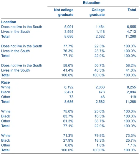
Table 2: Example of cross tabulation using panels Education Not college graduate College graduate Total Location
Does not live in the South 5,091 1,464 6,555
Lives in the South 3,595 1,118 4,713
Total 8,686 2,582 11,268
Does not live in the South 77.7% 22.3% 100.0%
Lives in the South 76.3% 23.7% 100.0%
Total 77.1% 22.9% 100.0%
Does not live in the South 58.6% 56.7% 58.2%
Lives in the South 41.4% 43.3% 41.8%
Total 100.0% 100.0% 100.0% Race White 6,192 2,063 8,255 Black 2,421 473 2,894 Other 73 46 119 Total 8,686 2,582 11,268 White 75.0% 25.0% 100.0% Black 83.7% 16.3% 100.0% Other 61.3% 38.7% 100.0% Total 77.1% 22.9% 100.0% White 71.3% 79.9% 73.3% Black 27.9% 18.3% 25.7% Other 0.8% 1.8% 1.1% Total 100.0% 100.0% 100.0% Source:nlsw88.dta
Because most documents are in portrait mode, rather than landscape, fitting multiple columns into tables is always a challenge. One answer provided bytaboutis therow block layout(layout(rb)) which makes for efficient use of page space. The underscores are used inclabto indicate blanks, and thereby remove redundant titles. This is partly because the format option (format(1p)) has added percent symbols to the data and the 100% indicate which are row percentages and which are column percentages.
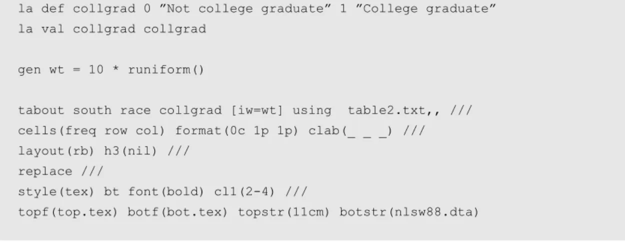
Stata code for Table 2
sysuse nlsw88, clear
la var south ”Location”
la def south 0 ”Does not live in the South” /// 1 ”Lives in the South”
la val south south
la var race ”Race”
la def race 1 ”White” 2 ”Black” 3 ”Other” la val race race
la def collgrad 0 ”Not college graduate” 1 ”College graduate” la val collgrad collgrad
gen wt = 10 * runiform()
tabout south race collgrad [iw=wt] using table2.txt,, /// cells(freq row col) format(0c 1p 1p) clab(_ _ _) /// layout(rb) h3(nil) ///
replace ///
style(tex) bt font(bold) cl1(2-4) ///
topf(top.tex) botf(bot.tex) topstr(11cm) botstr(nlsw88.dta)
Table 3: Same example but with rotation (LaTeX users)
Not college graduate College graduate Total Not college graduate College graduate Total Not college graduate College graduate Total Location
Does not live in the South 5,091 1,464 6,555 77.7% 22.3% 100.0% 58.6% 56.7% 58.2% Lives in the South 3,595 1,118 4,713 76.3% 23.7% 100.0% 41.4% 43.3% 41.8%
Total 8,686 2,582 11,268 77.1% 22.9% 100.0% 100.0% 100.0% 100.0% Race White 6,192 2,063 8,255 75.0% 25.0% 100.0% 71.3% 79.9% 73.3% Black 2,421 473 2,894 83.7% 16.3% 100.0% 27.9% 18.3% 25.7% Other 73 46 119 61.3% 38.7% 100.0% 0.8% 1.8% 1.1% Total 8,686 2,582 11,268 77.1% 22.9% 100.0% 100.0% 100.0% 100.0% N 1,714 532 2,246 Source:nlsw88.dta
This table shows how the column block layoutlayout(cb)can be used effectively. It does rely, however, on a LATEX option (label rotation) to fit everything into the limited horizontal space. (Users of word processors and spreadsheets can emulate this manually, using their cell ‘text direction’ menu item.) This table also shows the use of the ‘n’ option, with the sample counts placed at the bottom of the table, usingnpos(row).
Stata code for Table 3
sysuse nlsw88, clear
la var south ”Location”
la def south 0 ”Does not live in the South” /// 1 ”Lives in the South”
la val south south
la var race ”Race”
la def race 1 ”White” 2 ”Black” 3 ”Other” la val race race
la var collgrad ”Education”
la def collgrad 0 ”Not college graduate” 1 ”College graduate” la val collgrad collgrad
gen wt = 10 * runiform()
tabout south race collgrad [iw=wt] using table3.txt, ///
cells(freq row col) format(0c 1p 1p) layout(cb) h1(nil) h3(nil) npos(row) /// replace ///
style(tex) bt font(bold) rotate(60) ///
topf(top.tex) botf(bot.tex) topstr(15cm) botstr(nlsw88.dta)
LATEX users will need to make sure they have the following block of code in their document preamble if they wish to make use of the label rotation option.
LaTeX Code for rotation of table headings
\newcommand{\rot}[2]{\rule{1em}{0pt}% \makebox[0cm][c]{\rotatebox{#1}{\ #2}}}
Table 4: Same example illustrating noffset option
Not college graduate College graduate Total Not college graduate College graduate Total Not college graduate College graduate Total Location
Does not live in the South 5,062 1,581 6,643 76.2% 23.8% 100.0% 59.1% 58.5% 58.9% Lives in the South 3,507 1,123 4,630 75.7% 24.3% 100.0% 40.9% 41.5% 41.1%
Total 8,569 2,704 11,273 76.0% 24.0% 100.0% 100.0% 100.0% 100.0% Race White 6,124 2,115 8,239 74.3% 25.7% 100.0% 71.5% 78.2% 73.1% Black 2,353 544 2,898 81.2% 18.8% 100.0% 27.5% 20.1% 25.7% Other 91 45 136 66.8% 33.2% 100.0% 1.1% 1.7% 1.2% Total 8,569 2,704 11,273 76.0% 24.0% 100.0% 100.0% 100.0% 100.0% N 1,714 532 2,246 Source:nlsw88.dta
This table reproduces the last one, but shows the effect of thenoffsetoption. A common layout is frequencies first, then either column or row percentages, so it often makes more sense to ‘line up’ the n counts below the column percentages. Thenoffsetoption allows you to ‘shift’ the n counts along to line up under a column (or column block) of your choosing. In this example, thenoff(3)
shifts the n counts into the third block. If you weren’t using thelayout(cb)option and allowed the data to be in alternating columns (eg. freq row col freq row col etc), then the effect ofnoff(3)would be to place the n counts in the third alternating column: blank blank n blank blank n etc. Keep in mind thatnoffsetrefers to the data columns and rows, ignoring labels and headings (since to be precise, the first column always has labels in it). If you are using thenpos(row)ornpos(rb)options,
the same principles apply (just read ‘row’ instead of ‘column’ in the above explanation). (Note that from here on, I begin to introduce abbreviations for options which have appeared several times.)
Stata code for Table 4
sysuse nlsw88, clear
la var south ”Location”
la def south 0 ”Does not live in the South” /// 1 ”Lives in the South”
la val south south
la var race ”Race”
la def race 1 ”White” 2 ”Black” 3 ”Other” la val race race
la var collgrad ”Education”
la def collgrad 0 ”Not college graduate” 1 ”College graduate” la val collgrad collgrad
gen wt = 10 * runiform()
tabout south race coll [iw=wt] using table4.txt, ///
c(freq row col) f(0c 1p 1p) lay(cb) h1(nil) h3(nil) npos(row) /// noffset(3) ///
rep ///
style(tex) bt font(bold) rot(60) ///
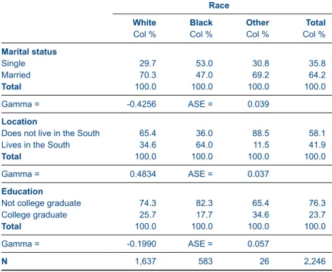
Table 5: Cross tabulation illustrating use of npos option and stats option
Race
White Black Other Total
Col % Col % Col % Col %
Marital status Single 29.7 53.0 30.8 35.8 Married 70.3 47.0 69.2 64.2 Total 100.0 100.0 100.0 100.0 Gamma = -0.4256 ASE = 0.039 Location
Does not live in the South 65.4 36.0 88.5 58.1
Lives in the South 34.6 64.0 11.5 41.9
Total 100.0 100.0 100.0 100.0
Gamma = 0.4834 ASE = 0.037
Education
Not college graduate 74.3 82.3 65.4 76.3
College graduate 25.7 17.7 34.6 23.7
Total 100.0 100.0 100.0 100.0
Gamma = -0.1990 ASE = 0.057
N 1,637 583 26 2,246
Source:nlsw88.dta
As withtabulate,taboutallows you to include various statistics at the bottom of your tables. Unliketabulate, however, only one statistic can be included with each table. Note the use of the
npos(row)option here to provide row counts. Stata code for Table 5
sysuse nlsw88, clear
la var south ”Location”
la def south 0 ”Does not live in the South” /// 1 ”Lives in the South”
la val south south
la var race ”Race”
la def race 1 ”White” 2 ”Black” 3 ”Other” la val race race
la var married ”Marital status” la def married 0 ”Single” 1 ”Married” la val married married
la var collgrad ”Education”
la def collgrad 0 ”Not college graduate” 1 ”College graduate” la val collgrad collgrad
gen wt = 10 * runiform()
tabout married south coll race using table5.txt, /// c(col) f(1) clab(Col_%) stats(gamma) npos(row) ///
rep ///
style(tex) bt font(bold) cl1(2-5) ///
topf(top.tex) botf(bot.tex) topstr(11cm) botstr(nlsw88.dta)
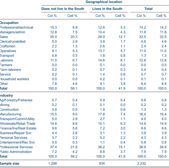
Table 6: Cross tabulation illustrating use of nlab and clab options
Geographical location
Does not live in the South Lives in the South Total
Col % Cell % Col % Cell % Col % Cell %
Occupation Professional/technical 15.3 8.9 12.6 5.3 14.2 14.2 Managers/admin 12.8 7.5 10.4 4.3 11.8 11.8 Sales 35.0 20.3 28.9 12.1 32.5 32.5 Clerical/unskilled 5.0 2.9 3.9 1.7 4.6 4.6 Craftsmen 2.2 1.3 2.6 1.1 2.4 2.4 Operatives 9.1 5.3 13.7 5.7 11.0 11.0 Transport 0.8 0.5 1.8 0.8 1.3 1.3 Laborers 11.5 6.7 14.6 6.1 12.8 12.8 Farmers 0.0 0.0 0.1 0.0 0.0 0.0 Farm laborers 0.2 0.1 0.7 0.3 0.4 0.4 Service 0.2 0.1 1.4 0.6 0.7 0.7 Household workers 0.0 0.0 0.2 0.1 0.1 0.1 Other 7.8 4.6 9.1 3.8 8.4 8.4 Total 100.0 58.1 100.0 41.9 100.0 100.0 Industry Ag/Forestry/Fisheries 0.7 0.4 0.9 0.4 0.8 0.8 Mining 0.2 0.1 0.1 0.0 0.2 0.2 Construction 0.8 0.5 1.9 0.8 1.3 1.3 Manufacturing 15.5 9.0 17.8 7.4 16.4 16.4 Transport/Comm/Utility 5.0 2.9 2.7 1.1 4.0 4.0 Wholesale/Retail Trade 14.8 8.6 15.1 6.3 14.9 14.9 Finance/Ins/Real Estate 9.6 5.6 7.2 3.0 8.6 8.6 Business/Repair Svc 4.4 2.6 3.1 1.3 3.9 3.9 Personal Services 3.7 2.2 5.2 2.2 4.3 4.3 Entertainment/Rec Svc 0.5 0.3 1.1 0.4 0.8 0.8 Professional Services 37.4 21.8 36.2 15.1 36.9 36.9 Public Administration 7.2 4.2 8.8 3.7 7.9 7.9 Total 100.0 58.2 100.0 41.8 100.0 100.0 Sample size 1,298 934 2,232 Source:nlsw88.dta
There are several ways to change labels intabout. A simple way is to temporarily recode vari-ables labels. In this example, south is redefined to ‘Geographical location’. When it comes to tabout’s‘built-in labels’, these can be changed with thenlabandclaboptions. Using thenlaboption allows you to change the default label for the n counts to something other than ‘N’, such as ‘Sample size’. For the column labels, theclaboption allows you change the default to anything you like. You do need to use underscores to indicate spaces in theclaboption. This departs from standard Stata practice, but is a much simpler method of indicating spaces.
Stata code for Table 6
sysuse nlsw88, clear
la def south 0 ”Does not live in the South” /// 1 ”Lives in the South”
la val south south
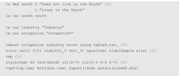
la var industry ”Industry” la var occupation ”Occupation”
tabout occupation industry south using table6.txt, ///
c(col cell) f(1) clab(Col_% Cell_%) npos(row) nlab(Sample size) /// rep ///
style(tex) bt font(bold) cl1(2-7) cl2(2-3 4-5 6-7) /// topf(top.tex) botf(bot.tex) topstr(14cm) botstr(nlsw88.dta)
Table 7: Same table illustrating column block layout option (cb) and dpcomma option
Location Does not live in the South Lives in the South
Total Does not live in the South
Lives in the South
Total
Column percentages Cell percentages
Occupation Professional/technical 15,3 12,6 14,2 8,9 5,3 14,2 Managers/admin 12,8 10,4 11,8 7,5 4,3 11,8 Sales 35,0 28,9 32,5 20,3 12,1 32,5 Clerical/unskilled 5,0 3,9 4,6 2,9 1,7 4,6 Craftsmen 2,2 2,6 2,4 1,3 1,1 2,4 Operatives 9,1 13,7 11,0 5,3 5,7 11,0 Transport 0,8 1,8 1,3 0,5 0,8 1,3 Laborers 11,5 14,6 12,8 6,7 6,1 12,8 Farmers 0,0 0,1 0,0 0,0 0,0 0,0 Farm laborers 0,2 0,7 0,4 0,1 0,3 0,4 Service 0,2 1,4 0,7 0,1 0,6 0,7 Household workers 0,0 0,2 0,1 0,0 0,1 0,1 Other 7,8 9,1 8,4 4,6 3,8 8,4 Total 100,0 100,0 100,0 58,1 41,9 100,0 Industry Ag/Forestry/Fisheries 0,7 0,9 0,8 0,4 0,4 0,8 Mining 0,2 0,1 0,2 0,1 0,0 0,2 Construction 0,8 1,9 1,3 0,5 0,8 1,3 Manufacturing 15,5 17,8 16,4 9,0 7,4 16,4 Transport/Comm/Utility 5,0 2,7 4,0 2,9 1,1 4,0 Wholesale/Retail Trade 14,8 15,1 14,9 8,6 6,3 14,9 Finance/Ins/Real Estate 9,6 7,2 8,6 5,6 3,0 8,6 Business/Repair Svc 4,4 3,1 3,9 2,6 1,3 3,9 Personal Services 3,7 5,2 4,3 2,2 2,2 4,3 Entertainment/Rec Svc 0,5 1,1 0,8 0,3 0,4 0,8 Professional Services 37,4 36,2 36,9 21,8 15,1 36,9 Public Administration 7,2 8,8 7,9 4,2 3,7 7,9 Total 100,0 100,0 100,0 58,2 41,8 100,0 Sample size 1.298 934 2.232 Source:nlsw88.dta
While Table 6 looks neat, cell percentages are more easily grasped as a block, so Table 7 duplic-ates the that table, but changes the layout to column block (layout(cb)). The table also illustrates one
of the more recent additions totabout: thedpcommaoption (which can be abbreviated todpc). This option replaces the period used for decimal points with a comma (and the thousands separator becomes a period, also called a full-stop).
Stata code for Table 7
sysuse nlsw88, clear
la var south ”Location”
la def south 0 ”Does not live in the South” /// 1 ”Lives in the South”
la val south south
la var industry ”Industry” la var occupation ”Occupation”
tabout occ ind south using table7.txt, ///
c(col cell) f(1) clab(Col_% Cell_%) npos(row) nlab(Sample size) /// lay(cb) dpcomma ///
rep ///
style(tex) bt font(bold) cl1(2-7) cl2(2-4 5-7) /// h3(& \multicolumn{3}{c}{Column percentages} & /// \multicolumn{3}{c}{Cell percentages} \\) ///
Basic tables with survey data
Table 8: Survey data showing row percentages with confidence intervals
Location
Does not live in the South Lives in the South Total
Row % 95% CI Row % 95% CI Row %
Education
Not college graduate (n=1,714) 58.8 [56.1,61.4] 41.2 [38.6,43.9] 100.0 College graduate (n=532) 59.6 [54.8,64.3] 40.4 [35.7,45.2] 100.0
Total(n=2,246) 59.0 [56.6,61.3] 41.0 [38.7,43.4] 100.0
Pearson: Uncorrected chi2(1) = 0.1124
Design-based F(1.00, 2245.00) = 0.0850 Pr = 0.771 Race White (n=1,637) 66.9 [64.3,69.5] 33.1 [30.5,35.7] 100.0 Black (n=583) 36.0 [31.7,40.6] 64.0 [59.4,68.3] 100.0 Other (n=26) 87.5 [63.8,96.5] 12.5 [3.5,36.2] 100.0 Total(n=2,246) 59.0 [56.6,61.3] 41.0 [38.7,43.4] 100.0
Pearson: Uncorrected chi2(2) = 182.1039
Design-based F(1.99, 4466.01) = 63.6567 Pr = 0.000
Marital status
Single (n=804) 58.7 [54.7,62.6] 41.3 [37.4,45.3] 100.0
Married (n=1,442) 59.1 [56.2,62.0] 40.9 [38.0,43.8] 100.0
Total(n=2,246) 59.0 [56.6,61.3] 41.0 [38.7,43.4] 100.0
Pearson: Uncorrected chi2(1) = 0.0390
Design-based F(1.00, 2245.00) = 0.0293 Pr = 0.864 Source:nlsw88.dta
When it comes to survey data, confidence intervals are easily handled bytabout. Thec(row ci)
option indicates that CIs are required, and the default settings include square brackets and a comma separator (though the former can be removed and the latter modified usingcibnoneandcisep( )). The
percentoption also turns proportions into percentages. In this example, the survey chi2 results are also included. Note the use of thenpos(lab)option to present n counts within the value labels of the vertical variables.
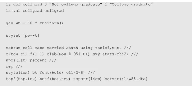
Stata code for Table 8
sysuse nlsw88, clear
la var south ”Location”
la def south 0 ”Does not live in the South” /// 1 ”Lives in the South”
la val south south
la var race ”Race”
la def race 1 ”White” 2 ”Black” 3 ”Other” la val race race
la var married ”Marital status” la def married 0 ”Single” 1 ”Married” la val married married
la def collgrad 0 ”Not college graduate” 1 ”College graduate” la val collgrad collgrad
gen wt = 10 * runiform()
svyset [pw=wt]
tabout coll race married south using table8.txt, /// c(row ci) f(1 1) clab(Row_% 95%_CI) svy stats(chi2) /// npos(lab) percent ///
rep ///
style(tex) bt font(bold) cl1(2-6) ///
topf(top.tex) botf(bot.tex) topstr(14cm) botstr(nlsw88.dta)
Table 9: Same table illustrating the new dpcomma option and the cisep option
Location
Does not live in the South Lives in the South Total
Row % 95% CI Row % 95% CI Row %
Education
Not college graduate (n=1.714) 57,2 [54,4-59,9] 42,8 [40,1-45,6] 100,0 College graduate (n=532) 58,9 [54,0-63,6] 41,1 [36,4-46,0] 100,0
Total(n=2.246) 57,6 [55,2-59,9] 42,4 [40,1-44,8] 100,0
Pearson: Uncorrected chi2(1) = 0,5001
Design-based F(1,00, 2245,00) = 0,3747 Pr = 0,540 Race White (n=1.637) 64,9 [62,2-67,5] 35,1 [32,5-37,8] 100,0 Black (n=583) 35,8 [31,5-40,4] 64,2 [59,6-68,5] 100,0 Other (n=26) 84,8 [60,6-95,3] 15,2 [4,7-39,4] 100,0 Total(n=2.246) 57,6 [55,2-59,9] 42,4 [40,1-44,8] 100,0
Pearson: Uncorrected chi2(2) = 156,3044
Design-based F(2,00, 4484,45) = 56,7473 Pr = 0,000
Marital status
Single (n=804) 56,2 [52,1-60,1] 43,8 [39,9-47,9] 100,0
Married (n=1.442) 58,3 [55,4-61,2] 41,7 [38,8-44,6] 100,0
Total(n=2.246) 57,6 [55,2-59,9] 42,4 [40,1-44,8] 100,0
Pearson: Uncorrected chi2(1) = 0,9755
Design-based F(1,00, 2245,00) = 0,7459 Pr = 0,388 Source:nlsw88.dta
Thedpcommaoption (abbreviated todpc) switches around periods and commas when it comes to decimal points. Obviously, for confidence intervals (as shown in Table 8) this can be confusing, so users will need to modify the CI separator. This is easily done with thecisepoption, which in this example makes use of a dash.
Stata code for Table 9
sysuse nlsw88, clear
la var south ”Location”
la def south 0 ”Does not live in the South” /// 1 ”Lives in the South”
la val south south
la var race ”Race”
la def race 1 ”White” 2 ”Black” 3 ”Other” la val race race
la var married ”Marital status” la def married 0 ”Single” 1 ”Married” la val married married
la var collgrad ”Education”
la def collgrad 0 ”Not college graduate” 1 ”College graduate” la val collgrad collgrad
gen wt = 10 * runiform()
svyset [pw=wt]
tabout coll race married south using table9.txt, /// c(row ci) f(1 1) clab(Row_% 95%_CI) svy stats(chi2) /// npos(lab) per dpc cisep(-) ///
rep ///
style(tex) bt font(bold) cl1(2-6) ///
Summary tables
Summary tables intaboutcan be as simple as the following table, where two variables (inc and can-didate) are cross-tabulated and the cell contents are based on the mean of another variable (pfrac). This is essentially the same as Stata’stablecommand. Note that thesumoption is required to indic-ate that this is a summary table.
Table 10: Simple twoway summary table illustrating a table of means
Candidate voted for, 1992
Family Income Clinton Bush Perot Total
% % % % <$15k 8.3 3.2 2.5 4.7 $15-30k 10.8 8.4 4.8 8.0 $30-50k 12.3 11.4 6.3 10.0 $50-75k 8.0 8.4 3.6 6.7 $75k+ 4.7 6.2 2.1 4.3 Total 8.8 7.5 3.9 6.7 Source:voter.dta
Stata code for Table 10
sysuse voter, clear
tabout inc candidat using table10.txt, /// c(mean pfrac) f(1) clab(%) sum ///
rep ///
style(tex) bt font(bold) cl1(2-5) ///
topf(top.tex) botf(bot.tex) topstr(12cm) botstr(voter.dta)
Table 11: Twoway summary table illustrating inter-quartile range
Inter-quartile range of weight
Repair Record 1978 Domestic Foreign Total N
1 3,100 3,100 2 2 3,354 3,354 8 3 3,442 2,010 3,299 30 4 3,532 2,208 2,870 18 5 1,960 2,403 2,323 11 Total 3,368 2,263 3,032 69 N 48 21 69 Source:auto.dta
Table 11 shows another example of a summary table, in this case the inter-quartile range. As mentioned earlier, this is but one of a large number of possible summary measures available with this option: N mean var sd skewness kurtosis sum uwsum min max count median iqr r9010 r9050 r7525 r1050 p1 p5 p10 p25 p50 p75 p90 p95 p99. Note thattaboutworks out that this is a twoway table and uses the last variable in the list (foreign) as the ‘horizontal’ variable.
Stata code for Table 11
sysuse auto, clear
tabout rep78 foreign using table11.txt, /// c(mean weight) f(0c) sum h3(nil) npos(both) /// rep ///
style(tex) bt font(bold) cl1(2-4) cltr1(.5em) ///
h1(& \multicolumn{3}{c}{\textbf{Inter-quartile range of weight}} \\) /// topf(top.tex) botf(bot.tex) topstr(10cm) botstr(auto.dta)
Table 12: Oneway summary table illustrating multiple summary measures
Mean Median MPG Weight (lbs) Length (in) Price Headroom (in) Car type Domestic (70%) 19.8 3,317.1 196.1 $4,782.50 3.5 Foreign (29%) 24.8 2,315.9 168.5 $5,759.00 2.5 Total (100%) 21.3 3,019.5 187.9 $5,006.50 3.0 Repair Record 1978 1 (2%) 21.0 3,100.0 189.0 $4,564.50 1.8 2 (11%) 19.1 3,353.8 199.4 $4,638.00 3.8 3 (43%) 19.4 3,299.0 194.0 $4,741.00 3.5 4 (26%) 21.7 2,870.0 184.8 $5,751.50 3.0 5 (15%) 27.4 2,322.7 170.2 $5,397.00 2.5 Total (100%) 21.3 3,032.0 188.3 $5,079.00 3.0 Source:auto.dta
This table illustrates a oneway summary table, but it is not necessary to specifyonewaybecause taboutworks this out from thecellscontents. It is essential, however, to include thesumoption to indicate that this is a summary table. While taboutonly allows a single summary measure in a twoway table (as shown in Tables 10 and 11 above), if oneway tables are chosentaboutdoes not limit the number of summary measures you can use (though page space might). Theclaboption also shows the use of underscores to indicate spaces. Finally, thenpos(tufte)option is shown.
Stata code for Table 12
sysuse auto, clear
tabout foreign rep78 using table12.txt, ///
c(mean mpg mean weight mean length median price median headroom) /// f(1c 1c 1c 2cm 1c) ///
clab(MPG Weight_(lbs) Length_(in) Price Headroom_(in)) /// sum npos(tufte) ///
rep ///
style(tex) bt cl2(2-4 5-6) cltr2(.75em 1.5em) ///
Summary tables with survey data
Table 13: Twoway summary table with standard errors
Education
Not college graduate College graduate Total
Mean wage SE Mean wage SE Mean wage SE Occupation Professional/technical (n=317) 9.73 (0.51) 12.31 (0.69) 10.91 (0.43) Managers/admin (n=264) 9.88 (0.68) 13.63 (0.94) 10.98 (0.56) Sales (n=726) 6.86 (0.23) 8.34 (0.57) 7.06 (0.22) Clerical/unskilled (n=102) 8.43 (1.13) 7.38 (1.49) 8.23 (0.96) Craftsmen (n=53) 6.75 (0.51) 11.00 (1.02) 7.17 (0.51) Operatives (n=246) 5.50 (0.28) 4.47 (1.47) 5.49 (0.28) Transport (n=28) 3.30 (0.33) 3.30 (0.33) Laborers (n=286) 4.88 (0.24) 6.45 (0.97) 4.99 (0.24) Farmers (n=1) 8.05 (0.00) 8.05 (0.00) Farm laborers (n=9) 2.98 (0.26) 2.51 (0.00) 2.94 (0.24) Service (n=16) 5.88 (0.69) 4.03 (0.00) 5.84 (0.67) Household workers (n=2) 6.46 (0.14) 6.46 (0.14) Other (n=187) 4.55 (0.39) 9.51 (0.40) 8.98 (0.39) Total(n=2,237) 6.94 (0.16) 10.40 (0.31) 7.78 (0.14) Location
Does not live in the South (n=1,304) 7.62 (0.22) 10.73 (0.40) 8.39 (0.20) Lives in the South (n=942) 6.01 (0.20) 9.92 (0.50) 6.93 (0.20)
Total(n=2,246) 6.94 (0.16) 10.40 (0.31) 7.77 (0.14) Race White (n=1,637) 7.43 (0.21) 10.19 (0.32) 8.13 (0.18) Black (n=583) 5.72 (0.18) 11.02 (0.85) 6.76 (0.24) Other (n=26) 6.84 (0.82) 11.80 (1.75) 8.89 (1.06) Total(n=2,246) 6.94 (0.16) 10.40 (0.31) 7.77 (0.14) Source:nlsw88
When it comes to survey data, you can include standard errors and confidence intervals in your summary tables. You are, however, restricted to a single measure: the mean. This is becausetabout uses Stata’ssvy:meancommand. This table illustrates one approach to presenting standard errors. Note that you must include both thesumoption and thesvyoption for tables like these.
Stata code for Table 13
sysuse nlsw88, clear
la var south ”Location”
la def south 0 ”Does not live in the South” /// 1 ”Lives in the South”
la val south south
la var race ”Race”
la def race 1 ”White” 2 ”Black” 3 ”Other” la val race race
la var collgrad ”Education”
la def collgrad 0 ”Not college graduate” 1 ”College graduate” la val collgrad collgrad
la var occupation ”Occupation”
gen wt = 10 * runiform()
svyset [pw=wt]
tabout occ south race coll using table13.txt, /// c(mean wage se) f(2 2) clab(Mean_wage SE) /// sum svy npos(lab) ///
rep ///
style(tex) bt cl1(2-7) font(bold) ///
topf(top.tex) botf(bot.tex) topstr(14cm) botstr(nlsw88)
Table 14: Twoway summary table with lower and upper CI bounds
Average wages according to location
Does not live in the South Lives in the South Total
Mean LB UB Mean LB UB Mean LB UB
Education
Not college graduate $7.74 $7.29 $8.19 $5.96 $5.61 $6.32 $7.00 $6.69 $7.30 College graduate $10.90 $10.07 $11.72 $9.78 $8.93 $10.63 $10.44 $9.84 $11.05 Total $8.51 $8.10 $8.91 $6.85 $6.50 $7.21 $7.82 $7.54 $8.10 Race White $8.54 $8.08 $8.99 $7.47 $6.97 $7.97 $8.17 $7.82 $8.51 Black $8.21 $7.35 $9.07 $5.87 $5.43 $6.30 $6.76 $6.32 $7.19 Other $10.03 $6.79 $13.28 $4.73 $0.74 $8.71 $9.50 $6.43 $12.57 Total $8.51 $8.10 $8.91 $6.85 $6.50 $7.21 $7.82 $7.54 $8.10 Source:nlsw88.dta
As well as a combined CI,taboutalso allows for separate lower bound and upper bound estim-ates using thelbanduboptions. This example also illustrates the money format (f(2m)). Currencies other than the $ can be specified using themoney( )option. In comparison to the earlier approach of relabelling the variable, in this example theh1option is used to change the default label for heading number 1. In the case of thetexoutput, the user must take responsibility for all of the LATEX code needed for this heading.
Stata code for Table 14
sysuse nlsw88, clear
la var south ”Location”
la def south 0 ”Does not live in the South” /// 1 ”Lives in the South”
la val south south
la var race ”Race”
la def race 1 ”White” 2 ”Black” 3 ”Other” la val race race
la var collgrad ”Education”