GEOCOMPUTATION TECHNIQUES FOR SPATIAL ANALYSIS: IS IT THE CASE FOR HEALTH DATA SETS?

GEOCOMPUTATION TECHNIQUES FOR SPATIAL ANALYSIS:

IS IT THE CASE FOR HEALTH DATA SETS?

GILBERTO CÂMARA

ANTÔNIO MIGUEL VIEIRA MONTEIRO

Image Processing Division, National Institute for Space Research, Brazil

Abstract

Geocomputation is an emerging field of research, which advocates the use of computational-intensive techniques such as neural networks, heuristic search and cellular automata for spatial data analysis. Since an increasing quantity of health-related data is collected in a geographical frame of reference, geocomputational methods show increasing potential for health data analysis. This paper presents a brief survey of the geocomputational field, including some typical applications and references for further reading.

1. Introduction

In recent years, the use of computer-based techniques for spatial data analysis has grown into an important scientific area, combining techniques from geographical information systems and emerging areas such as neurocomputing, heuristic search and cellular automata. In order to distinguish this new interdisciplinary area from the simple extension of statistical techniques for spatial data, some authors (Openshaw and Abrahart, 1996) have coined the term "geocomputation" to describe of the use of computer-intensive methods for knowledge discovery in physical and human geography, especially those that employ non-conventional data clustering and analysis

techniques. Lately, the term has been applied in a broader sense, to include spatial data analysis, dynamic modelling, visualisation and space-time dynamics (Longley, 1998).

This paper is a brief survey of geocomputational techniques. This survey should not be considered a comprehensive one, but attempts to portray a general idea of the concepts and motivation behind the brand name of "geocomputation". Our prime motivation on this paper is to draw the attention of the public health community to the new analytical possibilities offered by geocomputational techniques. We hope this discussion serves to widen their perceptions about new possibilities in spatial analysis of health data.

2. Motivations for Research on Geocomputation

Simply defined, geocomputation "is the process of applying computing technology to geographical problems". As Oppenshaw (1996) points out, "many end-users merely want answers to fairly abstract questions such as 'Are there any patterns, where are they, and what do they look like ?'". This definition, although generic, point to a number of motivating factors: the emergence of computerised data-rich environments, affordable computational power, and spatial data analysis and mining techniques.

The first motivation (data-rich environments) has come about by the massive data collection of socio-economical, environmental and health information, which is increasingly organised in computerised data bases, with geographical references such as census tracts or postcode. Even in Brazil, a country with limited tradition of public availability of geographical data, the 2000 Census is being described as the first such initiative where all data collection will be automated and georeferenced.

The second motivation (computational power) has materialised in two forms: the emergence of the GIS (geographical information systems) technology and of a set of algorithmically-driven techniques, such as neurocomputation, fuzzy logic and cellular automata.

The third motivation (data analysis and mining techniques) has been greatly driven by the use of spatial statistics data analysis techniques, a research topic of much importance in the last decades.

The broad nature of challenges and approaches to geocomputational research is perhaps best illustrated by considering four different, yet complementary approaches: computer-intensive pattern search, exploratory spatial data analysis, artificial intelligence techniques and dynamic modelling. This will be done in the next sections.

3. Focus 1 - Computer-Intensive Pattern Search

3.1GAM - The Geographical Analysis Machine

One of the most typical examples of the computer-intensive approach to geocomputation is the Geographical Analysis Machine (GAM), developed by Stan Openshaw and co-workers at the Centre for Computational Geographics at the University of Leeds. For a recent survey of the GAM, see Openshaw (1998). The following description is largely indebted to Turton (1998).

GAM is basically a cluster finder for point or small area data. Its purpose is to indicate evidence of localised geographical clustering, in cases where the statistical distribution of the phenomena is not known in advance. For the GAM algorithm, a cluster is as a localised excess incidence rate that is unusual in that there is more of

some variable than might be expected. Examples would include: a local excess disease rate, a crime hot spot, a unemployment black spot, unusually high positive residuals from a model, the distribution of a plant or surging glaciers or earthquake epicentres, pattern of fraud etc.

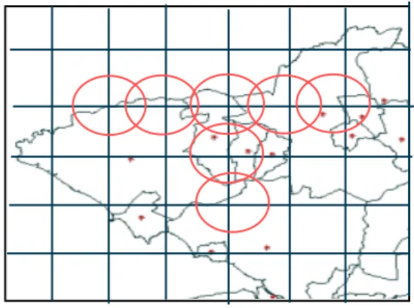
The basic idea of the GAM is very simple. Within the study region containing a spatial point pattern, GAM works by examining a large number of circles of varying sizes that completely cover the region of interest. The circles overlap to a large degree to allow for edge effects and to provide a degree of sensitivity analysis. Within each random circle, count the number of points and compare this observed value with an expected value based on an assumption about the process generating the point pattern (usually that it is random). Ideally, the population-at-risk should be used as a basis for generating the expected value, using for example a Poisson probability model with the observed mean and the population-at-risk within each circle. Once the statistical significance of the observed count within a circle has been examined the circle is drawn on a map of the region if it contains a statistically significant cluster of points. The process is repeated many times until a map is produced containing a set of circles centred on parts of the region where interesting clusters of points appear to be located.

Figure 1 – Two steps in the GAM algorithm – left, initial step with smaller circles; right, later step with bigger circles.

3.2A GAM Application for Infant Mortality in Rio

In Oppenshaw (1998) a strong case is made for the performance of the GAM algorithm for locating clusters of health diseases, including a comparison with other cluster finding techniques. To better assess and understand the potentials and limitations of GAM, the authors ran an example, using data from the study "Spatial Analysis Of Live-Born Profile And Socio-economic Conditions In Rio de Janeiro", conducted by D'Orsi and Carvalho (1997). This study assessed the spatial birth and socio-economic patterns in Rio de Janeiro city districts, aiming to identify the major groups of infant morbidity and mortality risk and the selection of the primary areas for preventive programs.

In order to apply the GAM algorithm, the values had to be converted from areal-related patterns to point variables. The authors selected some of the basic attributes used by D'Orsi and Carvalho, and converted each area unit (corresponding to a city district), to a point location, which received the value of the areal unit it represented, as illustrated by Figure 2. We ran the GAM algorithm on the values for the live-born

quality index for all neighbourhoods of Rio. As a result, GAM found three clusters of high values of this index, located approximately at the "Botafogo", "Barra da Tijuca" and "Ilha do Governador" regions, (Figure 3). As a comparison basis, the traditional cloropleth-map is shown in Figure 4, where the areal-based values are grouped by quintiles.

As expected, the results concentrated in what is perceived by the algorithm as 'extreme' events, disregarding cases which are not 'significant' enough. It should be noted that we have used the Rio birth patterns merely as an example to assess the behaviour of the GAM technique. We hope to motivate health researchers to apply the GAM techniques to problems closer to its original intended use, such as sets of epidemiological occurrences.

4. Focus 2 – Exploratory Spatial Data Analysis

4.1Local Spatial Statistics

Statistical data analysis currently is the most consistent and established set of tools to analyse spatial data sets. Nevertheless, the application of statistical techniques to spatial data faces an important challenge, as expressed in Tobler’s (1979) First Law of Geography: “everything is related to everything else, but near things are more related than distant things”. The quantitative expression of this principle is the effect of spatial dependence: the observed values will be spatially clustered, and the samples will not be independent. This phenomena, also termed spatial autocorrelation, has long being recognised as an intrinsic feature of spatial data, and measures such as the Moran coefficient and the semi-variogram plot have been used to assess the global association of the data set (Bailey and Gattrel, 1995).

Figure 2- Location of Rio de Janeiro city neighbourhoods. (source: D'Orsi and Carvalho, 1997)

Figure 3 - Clusters of high values APGAR index found by GAM.

Figure 4 – Grouping of values of APGAR index. (source: D'Orsi and Carvalho, 1997) 4 444,,11 -- 6633,,44 6 666,,44 -- 6699,,55 6 699,,55 -- 7744,,44 7 744,,44 -- 7777,,44 7 777,,44 -- 8833,,33 E Exxcclluuddeedd

Most spatial data sets, especially those obtained from geo-demographic and health surveys, not only possess global spatial autocorrelation, but also exhibit significant patterns of spatial instability, which is related to regional differentiations within the observational space. As stated by Anselin (1994), “the degree of non-stationary in large spatial data sets is likely to be such that several regimes of spatial association would be present”.

In order to assess the degree of spatial instability, a number of local spatial statistics indicators have been proposed, such as the Moran Local Ii (Anselin, 1995), the Moran scatterplot (Anselin, 1996) and the Gi and Gi* statistics (Ord and Getis, 1995). For a recent review, please see Getis and Ord, 1996. Although local spatial statistics can be seen as a branch of spatial statistics, they have been highly praised by geocomputational proponent Stan Oppenshaw: "it is absolutely fundamental that we can develop tools able to detect, by any feasible means, patterns and localised association that exist within the map." (Oppenshaw, 1996).

4.2Spatial Statistics as a Basis for Zoning: Social Exclusion/Inclusion in São Paulo In order to assess the validity of local spatial statistics, the authors have conducted a project to study the potential of such indicators as a basis for the design of administrative zoning systems for the city of São Paulo. As is well known, zone design is a major challenge for urban and regional planners, since it involves major decisions on how to distribute public resources.

The city of São Paulo is one of the world's largest and presents a major challenge to urban planners and public administrators. Given its present size (over 13 million inhabitants) and enormous socio-economic inequalities, the rational planning of the city

requires a careful division of the urban space into administrative regions that are homogenous by some objective criteria. Unfortunately, the current regional division of São Paulo has been driven by historical and political forces, and does not reflect a rational attempt to challenge the city's disparities.

As a basis for a zoning design for São Paulo, we have taken the "Social Exclusion/Inclusion Map of São Paulo", a comprehensive diagnosis of the city, co-ordinated by Prof. Aldaiza Sposati, of the Social Studies Group of the Catholic University of São Paulo. This map used 49 variables, obtained from Census data and local organisations, to quantify the social apartheid in 96 districts of São Paulo (Sposati, 1996).

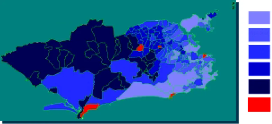
The main results of the "social exclusion/inclusion map" were indicators of social exclusion and of the disparity of the quality of life in São Paulo. Figure 6 shows the map of social exclusion index (Iex). In this map, the values vary between -1 (maximal social exclusion) and +1 (maximal social inclusion) with a value of 0 indicating the attainment of a basic standard of inclusion (Sposati, 1996). It can be noted from the map that 2/3 of the districts of São Paulo are below acceptable levels of living standards.

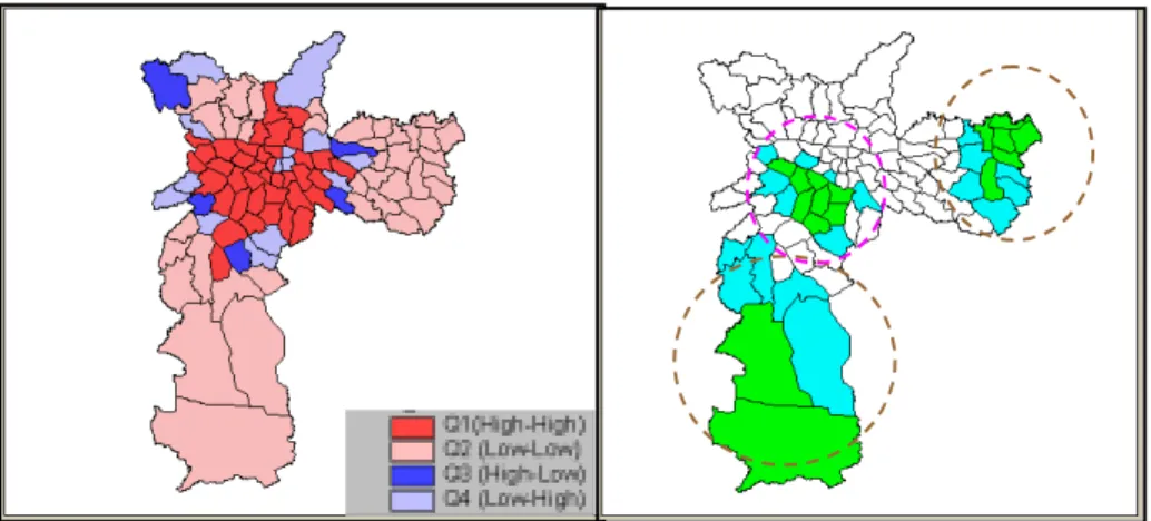
Taking the social exclusion index as a basis, the proposed task was to group the 96 districts into a set of administrative zones, each containing a significant number of districts, and homogeneous with respect to social exclusion status. We used two exploratory spatial analysis tools: the Moran Scatterplot Map (figure 6-left) and the local Moran index significance map (figure 6-right). The basis for these local spatial statistics indicators is the use of a neighbourhood or contiguity matrix W, whose elements are wij= 0 iff i and j are not neighbours, and non-zero otherwise.

The Moran scatterplot map is a tool for visualisation of the relationship between the observed values Z and the local mean values WZ, where Z indicates the array of attribute values (expressed as deviations from the mean), and WZ: is the array of local mean values, computed using matrix W. The association between Z and WZ can be explored to indicate the different spatial regimes associated to the data and display in a graphical form, as indicated by Figure 6 (left side). The Moran Scatterplot Map divides spatial variability into four quadrants:

• Q1 (positive values, positive local mean) and Q2 (negative values, negative local means): indicate areas of positive spatial association.

• Q3 (positive values, negative local means) and Q4 (negative values, positive local means): indicate areas of negative spatial association.

Since the Iex variable exhibits global positive spatial autocorrelation (Moran I = 0.65, significance= 99%), areas in quadrants Q3 and Q4 are interpreted as regions that do not follow the same global process of spatial dependence and these points indicate transitional regions between two different spatial regimes.

The local Moran index Ii is computed by multiplying the local normalised value zi, by the local mean (Anselin, 1995):

In order to establish a significance test for the local Moran index, Anselin (1995) proposes a pseudo-distribution simulation by permutation of the attribute values among the areas. Based on this pseudo-distribution, traditional statistical tests are used to indicate local index values with significance of 95% (1,96σ), 99% (2,54σ) and 99,9%

I

=

zi

Σ

Σ

(3,20σ). The 'significant' indexes are then mapped and posited as 'hot-spots' of local non-stationarity.

The local Moran index significance map indicated three ‘hot spots’, two of them related to low values of inclusion (located to the South and East of the city) and one related to high values of inclusion (located in the Centre of the city). These patterns correspond to the extreme regions of poverty and wealth in the city, and were chosen as “seeds” in the zoning procedure.

The remaining regions were defined interactively, taking into account the Moran scatterplot map, which clearly indicates a number of transition regions between the regions of Q1 and Q2 locations (to so-called “high-high” and “low-low” areas), some of whom are indicated by the green ellipses. These regions were grouped into separate zones. The work proceeded interactively, until a final zoning proposal was produced, which can be confronted with the current administrative regions (figure 7).

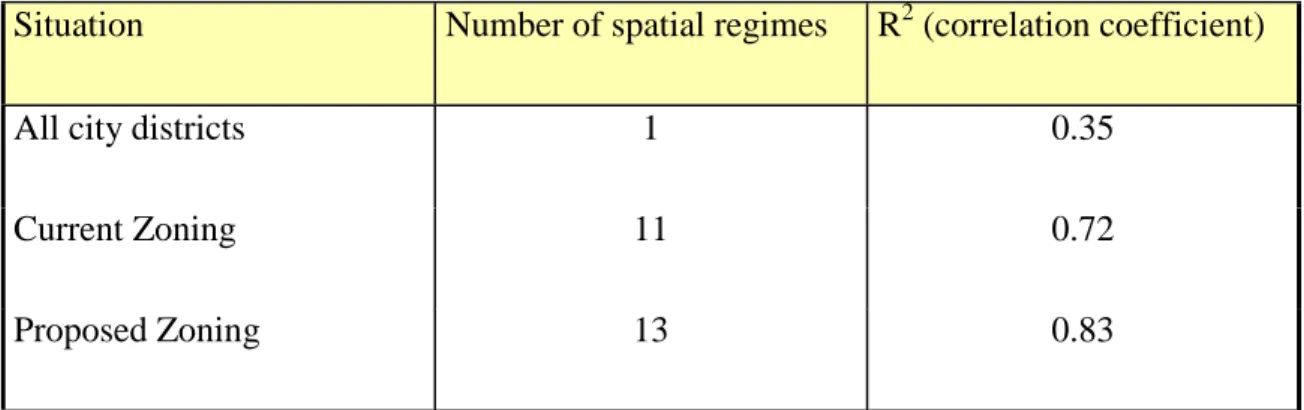
In order to assess the resulting map, a regression analysis was performed. This regression analyses the correlation between the percentage of houses with proper sewage facilities (as independent variable) and the percentage of people over 70 years of age (as dependent variable). The rationale behind this choice was that social deprivation is a serious impediment for a healthy living, as measured by the percentage of old-aged population. Three OLS (ordinary least squares) regression analyses were performed: the first, taking all districts of the city overall; a second one, using the current administrative division as separate spatial regimes; and the third, using the proposed new zoning as spatial regimes. The results as summarised in Table 1.

TABLE 1 – CORRELATION COEFFICIENTS FOR (OLD AGE, SEWAGE) REGRESSION IN SÃO PAULO

Situation Number of spatial regimes R2 (correlation coefficient)

All city districts 1 0.35

Current Zoning 11 0.72

Proposed Zoning 13 0.83

This results are a positive indication of the possible use of local spatial statistics as a basis for zoning procedures and show how indicators such as the social exclusion index of Sposati (1996) can be used as a support for urban planning.

5. Focus 3 – Neural Networks and Geographical Analysis

5.1Introduction

An Artificial Neural Network (ANN) is a computer paradigm that is inspired by the way the brain processes information. The key element of this paradigm is a processing system composed of a large number of highly interconnected elements (neurons) working in unison to solve specific problems. An ANN is configured for a specific application, such as pattern recognition or data classification, through a learning process (Gopal, 1998).

Figure 5 – Social Exclusion Index (Iex) in São Paulo (96 districts grouped in sextiles).

Figure 6 - Left: Moran Scatterplot Map for Iex in São Paulo. Right: Significant values of Local Moran Index (blue=95%; green=99%).

Figure 7 – Administrative Zones in São Paulo. Left – Current Division in 11 administrative regions. Right – Proposed division in 13 new regions.

In principle, ANNs can represent any computable function, i.e. they can do everything a normal digital computer can do. In practice, ANNs are especially useful for classification and function approximation and mapping problems which are tolerant of some imprecision and have lots of training data available. Almost any mapping between vector spaces can be approximated to arbitrary precision by feedforward ANNs (which are the type most often used in practical applications) if there are enough data and enough computing resources.

Given the capabilities of ANNs as exploratory tools in data-rich environments, there has been considerable interest in their use for spatial data analyse, especially in remote sensing image classification (Kannelopoulos, 1997; Leondes, 1997). Other geographical applications include: spatial interaction modelling (Oppenshaw, 1993; Gopal and Fischer, 1996) and classification of census data (Winter and Hewitson, 1994).

5.2 Neural Networks for Spatial Data Integration: A Economical-Ecological Zoning Application

To illustrate the potential of ANN for spatial data analysis, we have selected one example: the use of neural networks for the integration of multiple spatial information for an environmental zoning application (Medeiros, 1999). Although the chosen application does not involve health data, the integration procedure shown is relevant for heath-assessment applications, which involve multiple data sets as possible sources of epidemiological risk.

One of the more important problems in geographical data analysis is the integration of separate data sets to produce new spatial information. For example, in

health analysis, a researcher may be interested in assessing the risks associated to a disease (such as malaria) based on a combination of different conditions (land use and land cover, climatology, hydrological information, and distance to main roads and cities). These conditions can be expressed as maps, which are integrated into a common geographical database by means of GIS technology.

Once the data has been organised in a common geographical reference, the researcher needs to determine a procedure to combine these data sets. For example, a health researcher may posit the following inference: “calculate a malaria risk map based on disease incidence, climate, distance to cities and land cover, where the conditions are such that a region is deemed 'high risk for malaria' if it rains more that 1000 m/year and the landcover is 'inundated forest' and is located at less that 50 km from a city”.

The main problem with these map inference procedures is their ad-hoc, arbitrary nature: the researcher formulates hypothesis from previous knowledge and applies them to the data set. The process relies on inductive knowledge of the reality. Additionally, when the input maps have many different conditions, the definition of combinational rules for deriving the output may turn out to be difficult. For example, if input map has 8 different conditions (e.g., land cover classes) and five maps are to be combined, then 85 (=32768) different situations have to be taken into account.

There are two main alternative approaches to solve this problem. One is to use

fuzzy logic to combine the maps (Câmara et al., 2000). In this case, all input data is transformed into fuzzy sets (in a [0,1] scale) and a fuzzy inference procedure may be used. Alternatively, the use of neural network techniques aims at capturing the researcher's experience, without the need for the explicit definition of the inference

procedure. The application of neural networks to map integration can be done using the following steps:

1. Create a georeferenced data base with the input (conditional maps)

2. Select well-known regions as training areas. For these areas, indicate the desired output response (such as health risk).

3. Use these training areas as inputs to a neural-network learning procedure. 4. Using the trained network, apply the inference procedure for the entire study

region.

5. Evaluate the result and redo the training procedure, if necessary.

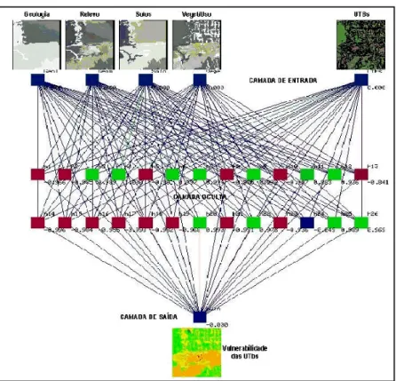
This idea was applied by Medeiros1 (1999) in his study of the integration of natural resources data as a basis for economical-ecological zoning in the Amazon region. Medeiros used five data sets as input: vegetation, geology, geomorphology, soils and remote sensing images. The intended output was a map of environmental vulnerability. The learning procedure is illustrated in Figure 8, where the diagram shows the five inputs and the output. Medeiros (1999) compared the result obtained by the neural network with a subjective, operator interpretation and found a very strong spatial coherence between the two maps, with the neural-produced one being more restrictive in terms of results that the subjective one. He concluded that it is feasible to apply neural networks as inference machines for integration of geographical data.

1

Figure 8 - Neural Network Training Procedure.

6. Focus 4 – Dynamical Modelling

The computer representation of geographical space in current GIS technology is essentially static. Therefore, one important research focus in geocomputation is aimed at producing models that combine the structural elements of space (geographical objects) to the processes that modify such space (human actions as they operate in time). Such models would liberate us from static visions of space (as centuries of map-making have conditioned us) and to emphasise the dynamic components as an essential part of geographical space.

This motivation has led to the use of cellular automata as a technique for simulation of urban and regional growth. Cellular automata (CA) are very simple dynamic spatial systems in which the state of each cell in an array depends on the

previous state of the cells within a neighbourhood of the cell, according to a set of transition rules. CA are very efficient computationally because they are discrete, iterative systems that involve interactions only within local regions rather than between all pairs of cells. The good spatial resolution that can thus be attained is an important advantage when modelling land use dynamics, especially for planning and policy applications (White and Engelen, 1997).

A conventional cellular automaton consists of: (a) an Euclidean space divided into an array of identical cells; (b) a cell neighbourhood; (c) a set of discrete cell states;

(d) a set of transition rules, which determine the state of a cell as a function of the states of cells in the neighbourhood; (e) discrete time steps, with all cell states updated simultaneously.

The application of CA to geographical systems was first proposed by Tobler (1979). More recently, a number of researchers have proposed modifications of the original CA idea to accommodate geographical constraints. The most important characteristic to be discarded is the homogeneous cell space, replaced by a space in which each cell has its own inherent set of attributes (as distinct from its single state) which represent its relevant physical, environmental, social, economic or institutional characteristics. These advances have been accompanied by an increase in the complexity of the models (Couclelis, 1997; White and Engelen, 1997).

This modification has allowed CA models to be linked both conceptually and practically with GIS. Once the CA is running on an inhomogeneous cell space (essentially identical to what would be found in a raster GIS), the CA may be thought of as a sort of dynamic GIS (Batty and Xie, 1994; Wu, 1998). At present, however, CA models developed in GIS remain simple, because GIS do not yet provide operators with

sufficient flexibility to define complex CA transition rules, and in addition they lack the simulation engines needed to run complex models at practical speeds. The more practical approach is to couple GIS to special purpose CA software modules, and possibly other models as well. White, Engelen and Uljee (1997) have developed several CA and CA based integrated models designed as prototypes of Spatial Decision Support Systems for urban and regional planning and impact analysis (demos of several of these models can be downloaded from http://www.riks.nl/RiksGeo/freestuff.htm).

7. In Conclusion: Geocomputation as a Set of Effective Procedures

This survey has examined some of the main branches of research in geocomputation and we conclude the paper with an attempt to provide a unified perspective of this new research field.

We propose that a unifying perspective for geocomputation is the emphasis on

algorithmical techniques. The rationale for this approach is that the emergence of data-rich spatial databases motivated a new set of techniques for spatial data analysis, most of them originally proposed under the general term of "artificial intelligence", such as neural networks, cellular automata and heuristic search.

Since there are fundamental differences in the perspectives of the set of techniques used by geocomputation, the only unification perspective is the

computational side: such techniques can be thought as a set of effective procedures, that, when applied to geographical problems, are bound to produce results. Whatever results are obtained need to be interpreted on the light of the basic assumptions of these techniques, and it may be extremely difficult to assign any traditional ‘statistical significance’ criteria to them.

Therefore, the authors propose a tentative definition: "Geocomputation is the use of a set of effective computing procedures to solve geographical problems, whose results are dependent on the basic assumptions of each technique and therefore are not strictly comparable."

In this view, geocomputation emphasises the fact that the structure and data-dependency inherent in spatial data can be used as part of the knowledge-discovery approaches and the choices involve theory as well as data. This view does not neglect the importance of the model-based approaches, such as the Bayesian techniques based on Monte Carlo simulation for the derivation of distribution parameters on spatial data. In fact, in this broader perspective, the use of Bayesian techniques that rely on computationally intense simulations can be considered a legitimate part of the geocomputational field of research.

In conclusion, what can public health researchers expect from geocomputation ? When used with discretion, and always bearing in mind the conceptual basis of each approach, techniques such as GAM, local spatial statistics, neural nets and cellular automata can be powerful aids to a spatial data analysis researcher, trying to discover patterns in space and relations between its components.

We hope this article serves as inspiration to health researchers, and hope to have extended their notions about what is possible in spatial data analysis.

Further Reading

For readers interested on more information on geocomputation, we provide a set of references, organised by topics. We suggest prospective readers to start with Longley (1998) and then proceed to his specific area of interest.

Reference Works on Geocomputation

ABRAHART,B. et al., 2000. Geocomputation Conference Series Home Page.

<http://www.ashville.demon.co.uk/geocomp/index.htm>

LONGLEY, P. (ed) Geocomputation: A Primer. New York, John Wiley and Sons, 1998.

OPENSHAW, S. and ABRAHART, R. J., 1996. Geocomputation. Proc. 1st International Conference on GeoComputation (Ed. Abrahart, R. J.), University of Leeds, UK, pp. 665-666.

OPENSHAW, S. and ABRAHART, R. J., 2000. Geocomputation. London, Taylor and Francis, 2000.

OPPENSHAW,S.; OPPENSHAW,C. 1997. Artificial Intelligence and Geography. New York, John Wiley.

Reference Works on Spatial Data Analysis

BAILEY,T.; GATTRELL, A 1995.. Spatial Data Analysis by Example London, Longman, 1995.

CARVALHO, M.S. (1997) Aplicação de Métodos de Análise Espacial na Caracterização de Áreas de Risco à Saúde . PhD Thesis in Biomedical Engineeriing, COPPE/UFRJ. <www.procc.fiocruz.br/~marilia>

Papers on GAM

OPENSHAW, S., 1998. Building automated Geographical Analysis and Exploration Machines. In: Geocomputation: A primer (Longley, P. A., Brooks, S. M. and Mcdonnell, B. (eds)), p95-115. Chichester, Macmillan Wiley.

TURTON, I., 1998. The Geographical Analysis Machine. Univ. of Leeds, Centre for Computational Geographics. <www.ccg.leeds.ac.uk/smart/gam/gam.html>

Papers on Exploratory Spatial Data Analysis

ANSELIN, L., 1995. Local indicators of spatial association - LISA. Geographical Analysis, 27:91-115.

ANSELIN, L.. 1996. The Moran scatterplot as ESDA tool to assess local instability in spatial association. In: Spatial Analytical Perspectives on GIS (Fisher, M.; Scholten, H. J.; Unwin, D., eds.) p. 111-126. London, Taylor & Francis.

GETIS, A., ORD J. K.; 1996. "Local spatial statistics: an overview". In: Spatial Analysis: Modelling in a GIS Environment. (LONGLEY,P.; BATTY,M., eds), pp. 261-277. New York, John Wiley.

OPENSHAW, S., 1997. Developing GIS-relevant zone-based spatial analysis methods. In: In: Spatial Analysis: Modelling in a GIS Environment. (LONGLEY,P.; BATTY,M., eds), pp. 55-73. New York, John Wiley.

ORD J. K.; GETIS, A., 1995. "Local spatial autocorrelation statistics: distributional issues and an application". Geographical Analysis, 27:286-306.

Papers on Neural Networks

KANELLOPOULOS, I. Use of Neural Networks for Improving Satellite Image Processing Techniques for Land Cover/Land Use Classification. European Commission, Joint Research Centre. <http://ams.egeo.sai.jrc.it/eurostat/Lot16-SUPCOM95/final-report.html>

GOPAL, S.; FISCHER, M., 1996. Learning In Single Hidden Layer Feedforward Neural Network Models: Backpropagation In A Spatial Interaction Modeling Context,

Geographical Analysis, 28 (1), 38-55, 1996.

GOPAL, S., 1998. Artificial Neural Networks for Spatial Data Analysis. In: NCGIA Core Curriculum in Geographic Information Science. (Kemp,K. ed.)

<http://www.ncgia.ucsb.edu/giscc/units/u188/u188.html>

HEWITSON, B. C.;CRANE, R. G. (eds). Neural Nets: Applications in Geography. Dordrecht. Kluwer Academic Publishers. 1994.

LEONDES,C. (ed), 1997. Image Processing and Pattern Recognition (Neural Network Systems Techniques and Applications Series, Vol 5). New York, Academic Press.

OPENSHAW, S., 1993. Modelling spatial interaction using a neural net, in M. M. Fischer and P. Nijkamp (eds) GIS Spatial Modeling and Policy, Springer, Berlin, pp. 147-164.

WINTER, K. E; HEWITSON, B. C., 1994. Self Organizing Maps - Application to Census. In: Neural Nets: Applications in Geography. (Hewitson, B. C.;Crane, R. G. (eds)).Dordrecht, Kluwer Academic Publishers.

Papers on Celular Automata for Spatial Analysis

BATTY, M. AND Y. XIE, 1994. "From Cells to Cities", Environment and Planning B, 21: pp. 531-548.

COUCLELIS, H., 1997, 'From cellular automata to urban models: new principles for model development and implementation', Environment and Planning B: Planning & Design, 24, 165-174.

O'SULLIVAN, D. 1999. Exploring the structure of space: towards geo-computational

Theory. In: Proc. IV International Conference on GeoComputation. Mary Washington College, VA, USA. <www.geovista.psu.edu/geocomp/geocomp99>.

TAKEYAMA, M.; COUCLELIS, H., 1997. 'Map dynamics: integrating cellular automata and GIS through Geo-Algebra', International Journal of Geographical Information Science, 11, 73-91.

TOBLER, W. R., 1979, 'Cellular geography', In: Philosophy in Geography, (Gale, S. and Olsson, G., eds.), pp. 379-386. Dordrecht, Holland, D Reidel Publishing Company. WHITE, R.; ENGELEN, G., 1993. "Cellular Dynamics and GIS: Modelling Spatial Complexity." Geographical Systems, vol. 1, 2.

WHITE R.; ENGELEN G., 1997 ‘Cellular Automata as the Basis of Integrated Dynamic Regional Modelling’ Environment and Planning B, Vol.24, pp.235-246. WHITE, R; ENGELEN, G.; ULJEE, I., 1997. “The use of constrained cellular automata for high-resolution modelling of urban land-use dynamics”. Environment and Planning B, Vol.24, pp.323-343.

Reference Works by Brazilian Researches

CÂMARA,G. (ed)., 2000. "Geoprocessamento: Teoria e Aplicações". April 2000. <http://www.dpi.inpe.br/gilberto/livro>. (In Portuguese).

D’ÓRSI,E.; CARVALHO,M.S. (1998). Perfil De Nascimentos No Município Do Rio De Janeiro - Uma Análise Espacial. Cadernos De Saúde Pública, 14(1):367-379. (In Portuguese).

MEDEIROS, 1999. Bancos de Dados Geográficos e Redes Neurais Artificiais: Tecnologias de Apoio à Gestão do Território. Tese de Doutorado em Geografia, USP.

<http://www.ltid.inpe.br/dsr/simeao/tesedout.html>

SPOSATI, A. 1996. Mapa da exclusão/inclusão social da cidade de São Paulo. São Paulo: EDUC.