New Kernels For Density and
Regression Estimation via
Randomized Histograms
Ruhi Ruhi
A thesis
in
The Department
of
Mathematics & Statistics
Presented in Partial Fulfillment of the Requirements
for the degree of Master of Science (Mathematics) at
Concordia University
Montreal, Quebec, Canada
August 2018
c
Concordia University
School of Graduate Studies
This is to certify that the thesis prepared By: Ruhi Ruhi
Entitled: New Kernels For Density and Regression Estimation via Randomized Histograms
and submitted in partial fulfillment of the requirements for the degree of
Master of Science (Mathematics)
complies with the regulations of the University and meets the accepted standards with respect to originality and quality.
Signed by the Final Examining Committee:
Chair Dr.Cody Hyndman
Examiner Dr.Yogendra P. Chaubey
Examiner Dr.Fr´ed´eric Godin
Thesis Supervisor Dr. Arusharka Sen
Approved by
Dr. Arusharka Sen, Graduate Program Director
August 28, 2018
ABSTRACT
New Kernels For Density and Regression Estimation via Randomized Histogram
Ruhi Ruhi
In early 20’s, the first person to notice the link between Random Forests (RF) and Kernel Methods, Leo Breiman (Breiman, 2000), pointed out that Random Forests grown using independent and identically distributed random variables in the tree construction is equivalent to kernels acting on true distribution. Later, Scornet (Scornet, 2016b) defined Kernel based Random Forest (KeRF) estimates and gave explicit expression for the kernels based on Centered RF and Uniform RF. In this paper, we will study the general expression for the connection function (kernel function) of an RF when splits/cuts are performed according to uniform distribution and also according to any general distribution. We also establish the consistency of KeRF estimates in both cases and their asymptotic normality.
Acknowledgements
I would like to acknowledge my indebtedness and render my warmest thanks to my supervisor, Dr. Arusharka Sen for his inspiration, direction, and the consistent help of my master’s studies. His friendly guidance and expert advice have been significant through all phases of the work.
I would also wish to express my gratitude to thesis committee Dr. Yogendra P. Chaubey and Dr. Fr´ed´eric Godin for valuable suggestions which have contributed greatly to the improvement of the thesis.
I humbly extend my thanks to faculty members of Department of Mathematics and Statistics, for providing excellent working conditions and graduate students who helped me through my studies at Concordia University.
And finally, I would like to thank my friends and family for their consistent support and inspiration throughout my studies.
Contents
1 Introduction 1
1.1 Framework. . . 2
1.1.1 Notations and definitions . . . 2
1.2 Basics of Kernel and Kernel based Random Forest(KeRF) . . . 4
1.2.1 Kernel based Random Forests (KeRF) . . . 4
1.2.2 Uniform KeRF . . . 6
1.2.2.1 Drawbacks of Scornet’s general expression of con-nection function Kkuf of Uniform Random Forest . . . 9
1.3 Outline of thesis. . . 9
2 Uniform Random Forest 11 2.1 Connection function for Scornet’s random forest . . . 11
2.2 Expression for Kernel by method of order statistics . . . 14
2.3 Asymptotic behavior of rn(x) . . . 16
2.3.1 Consistency and Asymptotic Normality of rn(x) . . . 16
3 Kernel for General partitioning distribution 27 3.1 Expression for the connection function KmG(x, z) . . . 27
3.2 Asymptotic behavior of rn(x) . . . 29
3.2.1 Consistency and Asymptotic Normality of rn(x) . . . 29
3.3 Finding the order of the bias . . . 34
4 Simulation Experiments 37 4.1 Density Estimation . . . 37
4.2 Regression Estimation . . . 44
5 Conclusion and Future work 52 References . . . 53
A R Codes 54 A.1 Uniform density estimator . . . 54
A.2 Non-Uniform Density Estimator . . . 57
A.2.1 Centered Density Estimator . . . 57
A.2.2 Non-Centered Density Estimator . . . 60
A.3 Uniform Regression Estimator . . . 63
A.4 Non-Uniform Regression Estimator . . . 66
A.4.1 Centered Regression Estimator . . . 66
1
Introduction
The Random Forest is one of the most popular and most powerful machine learning algorithms. It is basically a trademark term used for an ensemble learning method that consists of pooling together the estimates from many randomly generated decision trees. A decision tree (for classification, regression etc.) is a sequentially constructed partition of the space of input variable (co-variate)X. A tree estimate is the average (for regression) or mode (for classification) of all Y-values (output) that fall in the partition-cell containing a given input x.
Breiman’s work on CART (Classification and Regression Trees), ensemble estima-tor and Random Forest (RF) helped to bridge gap between statistics and com-puter science, particularly in the field of Machine Learning. Random Forests are exceptionally viable and progressively utilized measurable machine learning tech-niques. They give remarkable performances in many applied situations for classi-fication and regression problems as they run productively on extensive databases and also they can deal with huge number of input variable without variable dele-tion and have ability to deal with small sample sizes and high dimensional feature spaces. The corresponding R package randomForest can be freely downloaded on the CRAN website (http://www.cran.r-project.org/).
On the hypothetical side, the account of Random Forests are less indisputable and, in spite of their widespread use, little is known about their mathematical properties. However, recent studies have been done towards narrowing the gap
between theory and practice, which includes that of Denil et al.(2013) (Denil, Matheson, & Freitas,2013), who proved the consistency of a particular online for-est, Wager(2014) (Wager,2014) and Mentch and Hooker(2015) (Mentch & Hooker, 2016), who studied the asymptotic normality and Scornet et al.(2015) (Scornet, 2016a) who proved its consistency under appropriate assumptions.
1.1
Framework
Most of the following material is based on the papers Random Forest guided tour
(Biau & Scornet, 2016) and Random Forest and Kernel Methods (Scornet,2016b) by Erwan Scornet and G´erard Biau.
1.1.1
Notations and definitions
As explained by Scornet and Biau (Biau & Scornet,2016), the general structure of Random Forest is non-parametric regression estimation. Assume a training sample of sizen,D ={(X1, Y1), ...,(Xn, Yn)}of independent random variables distributed as independent prototype pair (X, Y) where E[Y2]<∞. An input random vector
X∈ X ⊂ Rp is observed and the goal is to predict the square integrable random response Y ∈R by estimating the regression function,
r(x) = E[Y |X =x].
The aim to use the data setDto construct an estimate rn :X →Rof the function
r. The regression function estimate rn is (mean squared error) consistent if
A random forest is a collection of M randomized regression trees (trees where target variable can take continuous values). Let rn(x,Θj) be the predicted value at point x for the j-th tree in the family, where Θ1,Θ2, ..,ΘM are independent random variables, distributed as generic random variable Θ, independent of the sampleD(of sample size n). These random variables represent the randomization procedure employed. The trees are combined to form the finite forest estimate
rM,n(x,Θ1, ..,ΘM) = 1 M M X j=1 rn(x,Θj). (1.1)
By the law of large numbers, the finite forest estimate approaches to infinite forest estimate (defining, r∞,n(x) = limM→∞rM,n(x,Θ)):
∀ x∈ [0,1]d, almost surely as M → ∞,
r∞,n(x) = E[rn(x,Θ)].
There are large variety of forests depending on how trees are grown and how the random variable Θ influences the tree construction. A basic framework to assess the theoretical properties of forests involves models in which partitions do not depend on the training set D. An example is the Centred Random Forests(Biau & Scornet, 2016), for which X = [0,1]d and has properties as follows:
(i) Samples are drawn without replacement;
(ii) at each node of each individual tree, a coordinate is uniformly chosen in {1,..., d} and,
(iii) a split is performed at the center of the node along the selected coordinate. The operations (ii)(iii) are recursively repeated k times, wherek ∈Nis a parame-ter. The algorithm stops when a binary tree withk levels is built, so that each tree has exactly 2kleaves in the end. The final estimation at the pointxis obtained by taking the average of Yi corresponding to the Xi in the cell of x. The parameter
k acts as a smoothing parameter that controls the size of the terminal node. Another example isUniform Forest, which is similar to Centred Forest except that once a split direction is chosen, the splits are made uniformly on the side of the cell, along the preselected co-ordinate (Arlot & Genuer, 2014).
1.2
Basics of Kernel and Kernel based Random
Forest(KeRF)
One way to break down the complexity of Random Forests is to express forest estimate as a kernel estimate, i.e., estimate rn which takes the form
rn(x) = Pn i=1YiKn(Xi,x) Pn i=1Kn(Xi,x) ,
where {(Xi, Yi); 1 ≤ i ≤n} is the training set, (Kn)k is the k-th kernel functions of the sequence of kernels ; n ∈N is parameter to be determined.
Note that the Kn doesn’t necessarily belongs to Nadaraya-Watson kernels family (Nadaraya, 1964) (Watson, 1964), which satisfy a translation-invariant homoge-neous property of the form Kh(x,z) = h1K((x−z)/h) for some smoothing pa-rameter h >0. The analysis of kernel is more complex, depending on the type of forest under investigation.
1.2.1
Kernel based Random Forests (KeRF)
For all x∈[0,1]d, we know (finite) random forest estimates satisfy
rM,n(x,Θ1, ...,ΘM) = 1 M M X j=1 n X i=1 Yi1Xi∈An(x,Θj) Nn(x,Θj) ! (1.2)
where An(x,Θj) is the cell containing x, determined by the random variable Θj and data set D and,
Nn(x,Θj) = n
X
i=1
1Xi∈An(x,Θj) is the number of data points in An(x,Θj) (Scornet, 2016b).
This equation (1.2) is true in particular for non-adaptive forests (i.e., forests built independently of data) as the quantity of observations in each cell cannot be controlled. For example, given two cases with N1
n(x,Θj) > Nn2(x,Θj) then by equation (1.2), r1
M,n(x,Θ1, ...,ΘM) < rM,n2 (x,Θ1, ...,ΘM). Thus cells containing smaller number of data points tends to have greater estimate than those with larger number of data points.
To solve this problem, Kernel based random forest(KeRF) estimates were defined, which takes the form:
e rM,n(x,Θ1, ...,ΘM) = PM j=1 Pn i=1Yi1Xi∈An(x,Θj) PM j=1Nn(x,Θj) (1.3)
To study more about KeRF, Scornet (Scornet, 2016b) proved a proposition for another form of KeRF estimates.
Proposition: Almost surely, for all x ∈[0,1]d,
e rM,n(x,Θ1, ...,ΘM) = Pn i=1YiKM,n(x,Xi) Pn j=1KM,n(x,Xj) , (1.4) where KM,n(x,z) = 1 M M X j=1 1z∈An(x,Θj). (1.5)
KM,n is connection function of the M finite forest.
(KM,n is a relative frequency of the set An containing x.)
Defining infinite KeRF estimates re∞,n as
e
r∞,n =limM→∞erM,n(x,Θ1, ...,ΘM).
A proposition for infinite forest estimate (i.e., when number of trees M tends to infinity) was proved by Scornet (Scornet, 2016b).
Note that the infinite random forests are said to be discrete (or continuous), if its corresponding connection function Kn is piece-wise constant (or continuous).
Proposition: Consider an infinite discrete or continuous forest. Then, almost surely, for all x,z ∈[0,1]d,
limM→∞KM,n(x,z) = Kn(x,z),
where
Kn(x,z) =PΘ[z∈An(x,Θ)]
Kn is called the connection function of infinite random forest. Thus, for all x∈ [0,1]d, e r∞,n(x) = Pn i=1YiKn(x,Xi) Pn j=1Kn(x,Xj) , (1.6)
Thus, infinite KeRF estimates are kernel estimates with kernel function equal to
Kn.
The denominator of KeRF estimate can be adjusted to obtain a density estimator as we shall see in Chapter 2 and Chapter 3.
1.2.2
Uniform KeRF
Uniform Random Forests were first studied by Biau et al.(Biau, Devroye, & Lugosi, 2008). In Uniform RF, the splits are drawn uniformly on the cell edges with no
prior on split location.
Using notation Kkuf to denote the connection function of uniform random forest of level k.
Scornet (Scornet,2016b) obtained an explicit expression Kkuf for connection func-tion for infinite uniform random forest as follows,
Proposition: For k ∈N and for all x ∈[0,1]d,
Kkuf(0,x) = X k1,..,kd; Pd l=1kl=k k! k1!...kd! 1 d !k × d Y m=1 1−xm km−1 X j=0 (−ln xm)j j! ! (1.7) with convention P−j=01 (−ln xm)j j! = 0.
The figure below represents the functions f1, f2,andf5 in two dimensions defined
by: fk : [0,1]×[0,1]→[0,1] z= (z1, z2)7→Kkuf 0,|z−(1 2, 1 2)| , where |z−x| = (|z1 −x1 |, ...,|zd−xd|).
Scornet(Scornet,2016b) also proved the expression of connection functionKkuf(x,z) for level k = 1,2 that has the form:
K1uf(x, z) = 1− |z−x| K2uf(x, z) = 1− |z−x|+|z−x|ln z 1−x , (1.8) for x, z ∈[0,1].
But for levels k > 2, the general expression of Kkuf couldn’t be derived. So, to overcome this difficulty, he replaced (x,z) → Kkuf(0,| z−x |) which is simpler way to build an invariant-by-translation version of uniform kernel Kkuf and the infinite uniform KeRF estimate, denoted by eruf
∞,n takes the
form-e r∞uf,n(x) = Pn i=1YiK uf k (0,|Xi−x|) Pn j=1K uf k (0,|Xj −x|) .
Later, the theorem below (Scornet,2016b) was proved to find consistency of infinite uniform KeRF estimates.
Theorem 1.1. Assuming
Y =r(X) +
where is a centred Gaussian noise, independent of X, with finite variance σ2 <
∞. Moreover, X is uniformly distributed on [0,1]d and r is Lipschitz of order 1.
Then, providing k → ∞ and n/2k → ∞, there exists a constant C
1 >0 such that
for all n >1 and for all x ∈[0,1]d,
E e r∞uf,n(x)−r(x) 2 ≤C1n−2/(6+3d log2)(logn)2.
1.2.2.1 Drawbacks of Scornet’s general expression of connection func-tion Kkuf of Uniform Random Forest
According to Scornet in his paper Random Forests and Kernel Methods(Scornet, 2016b), the general expression for connection function Kkuf(x,z);k > 2 of uni-form random forest is difficult to obtain. However, by using the method of order statistics, the general expression can be obtained by alternate partitioning scheme, which is shown in Chapter 2 of this thesis.
Also, the expression obtained in equation (1.8) by Scornet (Scornet,2016b) has a corrected form,
K2uf(x, z) = 1− |z−x|+|z−x|ln z(1−x), for x < z (1.9) which is also proved in Chapter 2.
1.3
Outline of thesis
The main objective of this paper is to find the explicit expression of kernel estimate for simplified randomization models, often called purely random forests. In this model, the domain of the explanatory variable x is partitioned m times using a random sample of sizen, independent of the dataD, from a distribution supported on the domain of x. Note that m = mn depends on n, the size of the data. We consider both uniform as well as non-uniform partitioning distributions. We establish consistency, expansions for bias and variance and asymptotic normality of the resulting estimators.
We denote the expression for the kernel for uniform partitioning as KU
m(x, z) and for non-uniform partitioning as KmG(x, z), where m is the number of splits.
We show in Chapter 2 that the expression for the kernel for uniform partitioning is
for x, z ∈[0,1]
KmU(x, z) = (1− |z−x|)m.
A similar expression for the kernel can be obtained in the multivariate case; the expression is of the form:
for x,z ∈[0,1]d KmU(x,z) = d Y i=1 (1− |zi−xi |)m.
The proof for multivariate case is straightforward and is not discussed in this thesis.
The rest of the thesis is organized as follows:
Chapter 2 is devoted to the results on kernel estimates for uniform partitioning and their asymptotic behavior. In Chapter 3, kernel estimates for general partitioning are presented along with their asymptotic properties and simulations are presented in Chapter 4.
2
Uniform Random Forest
In this chapter, we first obtain (Sec. 2.1) the correct expression for the uniform random forest kernel considered by Scornet (Scornet, 2016b) when the partition size is 4. As explained in Chapter 1, this kernel is not very convenient to work with, hence we do not pursue this approach. Instead, we derive the kernel for the alternative partitioning scheme proposed in Chapter 1 (Sec. 1.3: purely random forest). The rest of the chapter is devoted to studying properties of the resulting estimators.
2.1
Connection function for Scornet’s random
forest
Consider an interval [0,1] and let x, z∈ [0,1].
Let a point (say) u1 be drawn uniformly on (0,1), which partitions the interval
[0,1] in 2 intervals : (0,u1) and (u1,1).
The expression of kernel K1uf, already proved by Scornet (Scornet, 2016b), has form
Now, another point is drawn uniformly from one of the two sub-intervals and split is made at that point. This 2nd uniform split will be either in (0,u1) interval, if
x, z ∈(0,u1),creating 2 new intervals (0,u1u2) and (u1u2, u1) or in the interval (u1,
1), if x, z∈ [u1, 1], creating intervals (u1, u1+ (1−u1)u2) and (u1+ (1−u1)u2,1).
For any two points xand z in (0,1) (assuming w.l.o.g., x < z ), Probability that x and z are in same cell after 2 splits is K2uf(x, z),
K2uf(x, z) = P(max(x, z)< u1u2) +P(min(x, z)> u1u2, max(x, z)< u1)
+P(min(x, z)> u1, max(x, z)< u1+ (1−u1)u2)
+P(min(x, z)> u1+ (1−u1)u2)
=P(z < u1u2) +P(x > u1u2, z < u1) +P(x > u1, z < u1 + (1−u1)u2)
+P(x > u1+ (1−u1)u2)
=P(ln(z)< lnu1+lnu2) +P(lnx > lnu1+lnu2, lnz < lnu1)
+P(ln(1−x)< ln(1−u1), ln(1−z)> ln(1−u1) +ln(1−u2))
+P(ln(1−x)< ln(1−u1) +ln(1−u2))
[We know u∼unif(0,1) =⇒ −ln(u)∼exp(1)
(putting −lnui =Ti and−ln(1−ui) =Ti∗;i= 1,2)]
K2uf(x, z) = P(T1+T2 <−lnz) +P(T1+T2 >−lnx, T1 <−lnz) +P(T1∗ <−ln(1−x), T1∗+T2∗ >−ln(1−z)) +P(T1∗+T2∗ <−ln(1−x)) =P(S2 <−ln(z)) +P(S2 >−lnx, S1 <−lnz) +P(S1∗ <−ln(1−x), S2∗ >−ln(1−z)) +P(S2∗ <−ln(1−x)) whereSi =T1+..+Ti and Si∗ =T1∗+..+Ti∗
Also, we know that the random process {N(t); t≥0} such that
N(t) =max{n:Sn≤t} where Sn=T1+..+Tn; Ti ∼exp(λ) is a Poisson Process with rate λ.
K2uf =P(N(−ln(z))≥2) +P(N(−ln(z)) = 1, N(−lnx)−N(−lnz) = 0)
+P(N(−ln(1−x)) = 1, N(−ln(1−z))−N(−ln(1−x)) = 0) +P(N(−ln(1−x))≥2) [ whereN(t)∼P ois(t) andN(t1)−N(t2)∼P ois(t1−t2)]
= " ∞ X j=2 (−lnz)je lnz j! # + " elnz(−lnz)1 elnx−lnz(−lnx+lnz)0 # + " (−ln(1−x))1eln(1−x) eln(1−z)−ln(1−x)(−ln(1−z) +ln(1−x))0 # + " ∞ X j=2 eln(1−x)(−ln(1−x)) j j! # = " z ∞ X j=0 (−lnz)j j! − (−lnz)0 0! − (−lnz)1 1! # + " (−zlnz) x z # + " −(1−x).ln(1−x) 1−z 1−x # + " (1−x) ∞ X j=0 (−ln(1−x))j j! −(−ln(1−x)) 0−(−ln(1−x))1 # =z(e−lnz−1 +lnz)−xlnz−(1−z).ln(1−x) + (1−x) e−ln(1−x)−1 +ln(1−x) = 1−z+zlnz−xlnz−(1−z)ln(1−x) +x+ (1−x)ln(1−x) = 1−(z−x) + (z−x)lnz+ (z−x)ln(1−x) Hence, K2uf(x, z) = 1− |z−x|+|z−x|ln(z(1−x)) ; for x < z
This expression for k = 2 is the corrected form of the expression proved byErwan Scornet (Scornet, 2016b).
For k = 3 or more, the general expression of the connection function Kkuf(x,z) is difficult to obtain. So this method is not convenient for higher splits.
In the next section, we consider the partitioning scheme of apurely random forest. Recall that in this scheme a sample of size n of uniformly distributed points is used to create a partition of the interval [0,1]. We denote the resulting kernel by
KU
m(x, z) and corresponding estimate by rn(x).
2.2
Expression for Kernel by method of order
statistics
Observing KU
m(x, z) is the probability that x and z are connected in (infinite) random forest after m splits, the function KU
m characterizes the shape of the cells in the infinite forest.
Theorem 2.1. Let m∈Nand consider a uniform random forest of level m. Then, for all x, z ∈ [0,1],
KmU(x, z) = (1− |x−z|)m.
Proof. w.l.o.g., assume x < z.
Let m points be drawn independently from uniform distribution on (0,1) and let splits be made at those points for partitioning.
Assuming their order statistics to be
u(1) < u(2) < u(3) < .. < u(m).
We know that joint pdf of two order statistics, such that 16i < j 6m is f(i)(j)(x(i), x(j)) = m! (i−1)!(j −i−1)!(m−j)![F(x(i))] i−1 ×[F(x(j))−F(x(i))]j−i−1[1−F(x(j))]m−jf(x(i))f(x(j)), −∞< x(i)< x(j)<∞ Now, Considering P(x&z ∈j-th cell) =P(u(j) ≤x, z ≤u(j+1)) = Z x 0 Z 1 z fu(j),u(j+1)(u(j), u(j+1))du(j)du(j+1) = Z x 0 Z 1 z m! (j−1)!(j+ 1−j −1)!(m−j−1)![F(u(j))] j−1 ×[F(u(j+1))−F(u(j))]j+1−j−1[1−F(u(j+1))]m−j−1f(u(j))f(u(j+1)) = Z x 0 Z 1 z m! (j−1)!(m−j−1)!u j−1 (j) (1−u(j+1)) m−j−1du (j)du(j+1) = m! (j −1)!(m−j−1)! Z x 0 uj(j−)1du(j) Z 1 z (1−u(j+1))m−j−1du(j+1) = m! (j −1)!(m−j−1)! (u(j))j j x 0 .(1−u(j+1)) m−j m−j z 1 = m! j!(m−j)! x j(1−z)m−j We know, KU m(x,z) = P(x, z ∈ same cell).
P(x, z lies in same cell) = m X j= 1 m! (j−1)!(m−j)!x j (1−z)m−j = (x+ 1−z)m KmU(x, z) = (1− |z−x|)m Alternative proof:
w.l.o.g., assume x < z.
Let m points be drawn independently from uniform distribution on (0,1) and let splits be made at those points for partitioning. Let split point be denoted by u. Then,
P(x, z lies in same cell afterm splits) = (P[u∈(0, x)∪(z,1)])m = (1− |z−x|)m
2.3
Asymptotic behavior of
r
n(
x
)
We know that the estimate takes the form,
rn(x) = Pn i=1YiK U m(x, Xi) Pn i=1KmU(x, Xi) . As proved in Theorem 2.1, KmU(x, Xi) = (1− |x−Xi|)m. So, rn(x) := Nn(x) Dn(x) = m n Pn i=1Yi(1− |x−Xi|)m m n Pn i=1(1− |x−Xi|)m . (2.1) where Nn(x) = mn n P i=1
Yi(1− |x−Xi|)m and Dn(x) = m n
n
P
i=1
(1− |x−Xi|)m.
As we shall see below , the denominatorDn(x) converges to 2f(x). Therefore, the
Dn(x) can be modified to make it a density estimator (say) Fn(x) which is Dn2(x).
2.3.1
Consistency and Asymptotic Normality of
r
n(
x
)
In this section, we explore large-sample properties of our estimator. To accomplish this objective, we require some assumptions mentioned below:
Assumptions (A1):
• f(x) & r(x) are at least twice differentiable. • m=mn → ∞as n→ ∞ and
m n →0.
(In other words, m→0 but at slower rate than n−1)
Theorem 2.2. Assume (A1) holds. For x∈[0,1], Let Nn(x) = mn
n
P
i=1
Yi(1− |x−Xi|)m be a uniform kernel regression estimator and
Dn(x) = mn n
P
i=1
(1− |x−Xi|)m be a uniform kernel density estimator.
Then,the following convergence in probability holds:
rn(x) := Nn(x) Dn(x) = m n n P i=1 Yi(1− |x−Xi|)m m n n P i=1 (1− |x−Xi|)m → r(x)f(x) f(x) =r(x) (2.2)
Proof. : We will first consider E[Dn(x)] of equation (2.2),
E[Dn(x)] = E m n n X i=1 (1− |x−Xi|)m =mE(1− |x−X1 |)m =m Z 1 0 (1− |x−u|)mf(u)du =m Z x −(1−x) (1− |s |)mf(x−s)ds ; puttingx−u=s =m Z x −(1−x) (1− |s |)m f(x)−sf0(x) + s 2 2f 00 (x) +O(s3) ds
(using Taylor series expansions for f(x−s)) =m Z 0 −(1−x) (1 +s)m f(x)−sf0(x) + s 2 2f 00 (x) +O(s3) ds +m Z x 0 (1−s)m f(x)−sf0(x) + s 2 2f 00 (x) +O(s3) ds
= m m+ 1f(x) 2−xm+1−(1−x)m+1 + m m+ 1f 0 (x)x(1−x)m+1−(1−x)xm+1 + m (m+ 1)(m+ 2)f 0 (x)(1−x)m+2−xm+2 − m m+ 1 f00(x) 2 . (1−x)2xm+1+x2(1−x)m+1 − m (m+ 1)(m+ 2)f 00 (x)xm+2(1−x) +x(1−x)m+2 + m (m+ 1)(m+ 2)(m+ 3)f 00 (x)2−xm+3−(1−x)m+3. (2.3) Taking m→ ∞ , as 0< x < 1 & 0 <(1−x)<1 =⇒ xm →0 and (1−x)m →0 Hence, E[Dn(x)]→2f(x) Next, Taking E[Nn(x)] of equation (2.2), E[Nn(x)] =E m n n X i=1 Yi(1− |x−Xi|)m =mE(Y1(1− |x−X1 |)m) =m Z Z v(1− |x−u|)mf(u, v)dudv =m Z 1 0 (1− |x−u|)m Z vf(v |u)dv | {z } =r(u) f(u)du ; putting x−u=s =m Z x −(1−x) (1− |s|)mf(x−s)r(x−s)ds =m Z 0 −(1−x) (1 +s)mf(x−s)r(x−s)ds+m Z x 0 (1−s)mf(x−s)r(x−s)ds =m Z 0 −(1−x) (1 +s)m f(x)−sf0(x) + s 2 2f 00 (x) +O(s3) r(x)−sr0(x) + s 2 2r 00 (x) +O(s3) ds +m Z x 0 (1−s)m f(x)−sf0(x) + s 2 2f 00 (x) +O(s3) r(x)−sr0(x) + s 2 2r 00 (x) +O(s3) ds
= m m+ 1f(x)r(x) 2−xm+1−(1−x)m+1 + m m+ 1(f(x)r(x)) 0 x(1−x)m+1−(1−x)xm+1 + m (m+ 1)(m+ 2)(f(x)r(x)) 0 (1−x)m+2−xm+2 − m 2(m+ 1)(f(x)r(x)) 00 x2(1−x)m+1+ (1−x)2xm+1 − m (m+ 1)(m+ 2)(r(x)f(x)) 00 x(1−x)m+2−(1−x)xm+2 + m (m+ 1)(m+ 2)(m+ 3)(f(x)r(x)) 00 2−xm+3−(1−x)m+3 (2.4) Taking m→ ∞, as 0 < x < 1 & 0 <(1−x)< 1 =⇒ xm →0 and (1−x)m →0 E[Nn(x)]→2f(x)r(x) Hence, E[Nn(x)] E[Dn(x)] → 2r(x)f(x) 2f(x) =r(x)
Further,we will show the consistency of our estimate. For that we will prove V ar[Nn(x)]→0 and V ar[Dn(x)]→0.
V ar[Dn(x)] =V ar m n n X i=1 (1− |x−Xi|)m = m 2 n V ar(1− |x−X1 |) m = m n h mE(1− |x−X1 |)2m− 1 m(mE(1− |x−X1 |) m)2i = m n h m Z 1 0 (1− |x−u|)2mf(u)du− 1 m(mE(1− |x−X1 |) m)2i = m n h m Z x −(1−x) (1− |s|)2mf(x−s)ds− 1 m(mE(1− |x−X1 |) m)2i
= m n h m Z 0 −(1−x) (1 +s)2m f(x)−sf0(x) + s 2 2f 00 (x) +O(s3) ds +m Z x 0 (1−s)2m f(x)−sf0(x) + s 2 2f 00 (x) +O(s3) ds − 1 m(mE(1− |x−X1 |) m)2i = m n " m 2m+ 1f(x)(2−x 2m+1− (1−x)2m+1) + m 2m+ 1f 0 (x)(x(1−x)2m+1−(1−x)x2m+1) + m (2m+ 1)(2m+ 2)f 0 (x)((1−x)2m+2−x2m+2) − m 2(2m+ 1)f 00 (x)(x2(1−x)2m+1+ (1−x)2x2m+1) − m (2m+ 1)(2m+ 2)f 00 (x)((1−x)x2m+2+x(1−x)2m+2) + m (2m+ 1)(2m+ 2)(2m+ 3)f 00 (x)(2−x2m+3−(1−x)2m+3) − 1 m(mE(1− |x−X1 |) m)2 #
From assumption (A1),
m→ ∞ as n→ ∞ and mn →0 as 0 < x < 1 & 0 <(1−x)< 1 =⇒ xm →0 and (1−x)m →0 Thus, V ar[Dn(x)]→0 Now, V ar[Nn(x)] =V ar m n n X i=1 Yi(1− |x−Xi|)m = m 2 n V Y1(1− |x−X1 |)m = m n h mE(Y12(1− |x−X1 |)2m)− 1 m{mE(Y1(1− |x−X1 |) m)}2i
= m n " m Z Z v2(1− |x−u|)2mf(u, v)dudv− 1 m{mE(Y(1− |x−X1 |) m)}2 | {z } A # = m n " m Z Z v2(1− |x−u|)2mf(v|u)f(u)dudv−A # = m n " m Z x −(1−x) (1− |s |)2mf(x−s) Z v2f(v|x−s)dv | {z } =ζ(x−s) ds−A # h define: Z y2f(y|x)dy =ζ(x)i = m n " m Z x −(1−x) (1− |s |)2mf(x−s)ζ(x−s)ds−A # = m n " m Z x −(1−x) (1− |s |)2m f(x)−sf0(x) + s 2 2f 00 (x) +O(s3) × ζ(x)−sζ0(x) + s 2 2ζ 00 (x) +O(s3) ds−A # = m n " m Z 0 −(1−x) (1 +s)2m f(x)−sf0(x) + s 2 2f 00 (x) +O(s3) × ζ(x)−sζ0(x) + s 2 2ζ 00 (x) +O(s3) ds +m Z x 0 (1−s)m f(x)−sf0(x) + s 2 2f 00 (x) +O(s3) × ζ(x)−sζ0(x) + s 2 2ζ 00 (x) +O(s3) ds−A # = m n " m 2m+ 1(f(x)ζ(x))(2−x 2m+1−(1−x)2m+1) + m 2m+ 1(f(x)ζ(x)) 0 (x(1−x)2m+1−(1−x)x2m+1) + m (2m+ 1)(2m+ 2)(f(x)ζ(x)) 0 ((1−x)2m+2−x2m+2) + m 4m+ 2(f(x)ζ(x)) 00 ((1−x)2x2m+1−x2(1−x)2m+1) − m (2m+ 1)(2m+ 2)(f(x)ζ(x)) 00 ((1−x)x2m+2+x(1−x)2m+2) + m (2m+ 1)(2m+ 2)(2m+ 3)(f(x)ζ(x)) 00 (2−x2m+3−(1−x)2m+3)−A #
From assumption (A1), m→ ∞ as n→ ∞ and mn →0 as 0 < x < 1 & 0 <(1−x)< 1 =⇒ xm →0 and (1−x)m →0 Thus, V ar[Nn(x)]→0
which implies that Nn(x)−E[Nn(x)]→0 in probability and
Dn(x)−E[Dn(x)]→0 in probability. Thus,
rn(x)→r(x) in probability hence, is consistent.
Next, we study the asymptotic normality of our regression estimator Nn(x) and density estimator Dn(x).
Theorem 2.3. Let m∈N be number of splits and n be the sample size. Assuming (A1) holds, we have
r n m Nn(x)−E(Nn(x)) Dn(x)−E(Dn(x)) −→ N2 0 0 , f(x)ζ(x) f(x)r(x) f(x)r(x) f(x) ! where ζ(x) = E[Y2 |X =x]. Proof. Consider pn m E[Nn(x)]−2f(x)r(x) and pn m E[Dn(x)]−2f(x)
Recall equation (2.4) r n m E[Nn(x)]−2f(x)r(x) = r n m " m m+ 1f(x)r(x) 2−xm+1−(1−x)m+1 + m m+ 1(f(x)r(x)) 0 x(1−x)m+1−(1−x)xm+1 + m (m+ 1)(m+ 2)(f(x)r(x)) 0 (1−x)m+2−xm+2 − m 2(m+ 1)(f(x)r(x)) 00 x2(1−x)m+1+ (1−x)2xm+1 − m (m+ 1)(m+ 2)(r(x)f(x)) 00 x(1−x)m+2−(1−x)xm+2 + m (m+ 1)(m+ 2)(m+ 3)(f(x)r(x)) 00 2−xm+3−(1−x)m+3 −2f(x)r(x) # Taking m→ ∞, as 0 < x < 1 & 0 <(1−x)< 1 =⇒ xm →0 and (1−x)m →0 This implies, r n m E[Nn(x)]−2f(x)r(x) →0
Similarly, Recall equation (2.3)
r n m E[Dn(x)]−2f(x) = r n m " m m+ 1f(x) 2−xm+1−(1−x)m+1 + m m+ 1f 0 (x)x(1−x)m+1−(1−x)xm+1 + m (m+ 1)(m+ 2)f 0 (x)(1−x)m+2−xm+2 − m m+ 1 f00(x) 2 . (1−x)2xm+1+x2(1−x)m+1 − m (m+ 1)(m+ 2)f 00 (x) xm+2(1−x) +x(1−x)m+2 + m (m+ 1)(m+ 2)(m+ 3)f 00 (x)2−xm+3−(1−x)m+3−2f(x) #
Taking m→ ∞, as 0 < x < 1 & 0 <(1−x)< 1 =⇒ xm →0 and (1−x)m →0 This implies, r n m E[Dn(x)]−2f(x) →0 Consider, r n m rn(x)−r(x) = r n m Nn(x) Dn(x) −r(x) = r n m " Nn(x)−E(Nn(x)) Dn(x) − E(Nn(x)) E(Dn(x)) [Dn(x)−E(Dn(x))] Dn(x) +E(Nn(x)) E(Dn(x)) −r(x) # (2.5) Next, we define σ11(x) := n mV ar[Nn(x)]→f(x)ζ(x) σ22(x) := n mV ar[Dn(x)]→f(x) σ12(x) =σ21(x) := n mCov[Nn(x), Dn(x)] Cov[Nn(x), Dn(x)] = Cov m n n X i=1 Yi(1− |x−Xi|)m, m n n X j=1 (1− |x−Xj |)m = m 2 n2 X i X j cov(Yi(1− |x−Xi|)m,(1− |x−Xj |)m) = m 2 n2 n X i=j=1 cov(Yi(1− |x−Xi|)m,(1− |x−Xi|)m) + m 2 n2 X i6=j cov(Yi(1− |x−Xi|)m,(1− |x−Xj |)m) | {z } =0 (as Xi0s are i.i.d) = m 2 n " E(Y1(1− |x−X1 |)2m)−E(Y1(1− |x−X1 |)m)E(1− |x−X1 |)m #
= m 2 n " Z Z v(1− |x−u|)2mf(u, v)dudv−E(Y1(1− |x−X1 |)m)E(1− |x−X1 |)m # = m 2 n " Z (1− |x−u|)2m Z vf(v |u)dv | {z } =r(u) f(u)du−E(Y1(1− |x−X1 |)m)E(1− |x−X1 |)m # = m 2 n " Z 1 0 (1− |x−u|)2mf(u)r(u)du− E(Y1(1− |x−X1 |)m)E(1− |x−X1 |)m # = m 2 n " Z x −(1−x) (1− |s |)2mf(x−s)r(x−s)ds− E(Y1(1− |x−X1 |)m)E(1− |x−X1 |)m # (putting x−u=s) = m 2 n " Z 0 −(1−x) (1 +s)2m f(x)−sf0(x) + s 2 2f 00 (x) +O(s3) × r(x)−sr0(x) + s 2 2r 00(x) +O(s3) ds− Z x 0 (1−s)2m f(x)−sf0(x) + s 2 2f 00(x) +O(s3) × r(x)−sr0(x) + s 2 2r 00 (x) +O(s3) ds−E(Y1(1− |x−X1 |)m)E(1− |x−X1 |)m # = m n m 2m+ 1f(x)r(x)(2−x 2m+1−(1−x)2m+1) + m 2m+ 1(f(x)r(x)) 0 [x(1−x)2m+1−x2m+1(1−x)] + m (2m+ 1)(2m+ 2)(f(x)r(x)) 0[(1−x)2m+2−x2m+2] − m 2(2m+ 1)(f(x)r(x)) 00 ((1−x)2x2m+1+x2(1−x)2m+1] − m (2m+ 1)(2m+ 2)(f(x)r(x)) 00 [x(1−x)2m+2+ (1−x)x2m+2] + m (2m+ 1)(2m+ 2)(2m+ 3)(f(x)r(x)) 00 [2−x2m+3−(1−x)2m+3] − 1 m(mE(Y1(1− |x−X1 |) m))(m E(1− |x−X1 |)m) # Letting m→ ∞ =⇒ σ12= n mCov[Nn(x), Dn(x)]→f(x)r(x)
Thus, byCram´er-Wold device the joint convergence stated in theorem 2.3 follows.
Z2 ∼ N(0, σ22), the limiting distribution of density estimate Dn(x). Then, by Central Limit Theorem,
r n m Nn(x)−E(Nn(x)) d − → Z1 r n m Dn(x)−E(Dn(x)) d − → Z2
Thus, applying Slutsky’s Theorem to equation (2.5),
r n m rn(x)−r(x) d − → Z1 2f(x)− r(x) 2f(x)Z2 since Dn(x)→2f(x) ,Nn(x)→2f(x)r(x) and EE((NDnn((xx)))) →r(x). Thus, r n m rn(x)−r(x) ∼ N 0, σ11 4f2(x) −2 r(x) 4f2(x)σ12+ r2(x) 4f2(x)σ22 ∼ N 0,f(x)ζ(x) 4f2(x) −2 r2(x)f(x) 4f2(x) + r2(x)f(x) 4f2(x) ∼ N 0, 1 4f(x)(ζ(x)−r 2 (x)) =N 0,V ar[Y |X =x] 4f(x) and r n m Nn(x)−E(Nn(x)) Dn(x)−E(Dn(x)) −→ N2 0 0 , σ11(x) σ12(x) σ21(x) σ22(x) ! −→ N2 0 0 , f(x)ζ(x) f(x)r(x) f(x)r(x) f(x) !
3
Kernel for General partitioning
distri-bution
Recall that in Chapter 2,mpoints are drawn uniformly on (0,1) and splits are made at those points. In this chapter, m points are drawn from a general distribution
G(·) and splits are performed at those points. We will study the expression for the connection function and show that the corresponding estimate rn(x) is consistent for r(x). We denote the resulting kernel by KG
m(x, z).
3.1
Expression for the connection function
K
mG(
x, z
)
We know that KmG(x, z) is the probability that x and z are connected in random forests after m splits.
Theorem 3.1. Let m ∈ N. Then, for any two points x and z, the connection function of a finite forest of level m takes the form:
KmG(x, z) = (1− |G(z)−G(x)|)m
where G(·) is the distribution function of split points.
Take order statistics of splits to be
y(0) 6y(1) 6y(2)..6y(m)
where y(i) ∼ general distribution function G with densityg.
w.l.o.g., Assuming x < z.
Letx, z ∈ [y(i), y(i+1)] for some i,
P(x, z∈ith cell) =P(y(i) 6x < z 6y(i+1)) = P(yi 6x, z 6y(i+1)) = Z x −∞ Z ∞ z gY(i),Y(i+1)(y(i), y(i+1))dy(i)dy(i+1) = Z x −∞ Z ∞ z m! (i−1)!(i+ 1−i−1)!(m−i−1)![G(y(i))] i−1 ×[G(y(i+1))−G(y(i))]i+1−i−1[1−G(y(i+1))]m−i−1.g(y(i)).g(y(i+1))dy(i)dy(i+1) = m! (i−1)!(m−i−1)! Z x −∞ (G(y(i))i−1g(y(i))dy(i) | {z } = h(G(y (i)))i i ix −∞ Z ∞ z (1−G(y(i+1)))m−i−1g(y(i+1))dy(i+1) | {z } = h (1−G(y(i+1)))m−i m−i iz ∞ = m! i!(m−i)!.(G(x)) i(1−G(z))m−i
P(x, z lies in same cell after m splits) = m X i=0 m! i!(m−i)!.(G(x)) i(1−G(z))m−i = (1−G(z) +G(x))m KmG(x, z) = (1− |G(z)−G(x)|)m Alternative proof: w.l.o.g., assume x < z.
Letmpoints be chosen from any distribution with c.d.f. G(x) and splits are made at thesem points. Denoting split point byy.
Then,
P(x, z lies in same cell afterm splits) = (P[y∈(−∞, x)∪(z,∞)])m = (1− |G(z)−G(x)|)m.
3.2
Asymptotic behavior of
r
n(
x
)
In the above section, we find that the connection function has the form:
KmG(x, z) = (1− |G(x)−G(z)|)m.
Therefore, the estimate becomes:
rn(x) := Nn(x) Dn(x) = m n Pn i=1Yi(1− |G(x)−G(Xi)|) m m n Pn i=1(1− |G(x)−G(Xi)|)m . (3.1) where Nn(x) = mn n P i=1 Yi(1− |G(x)−G(Xi)|)m and Dn(x) = mn n P i=1 (1− |G(x)−G(Xi)|)m.
As we shall see below, the denominator Dn(x) converges to 2fg((xx)). Therefore, the Dn(x) can be modified to make it a density estimator (say) Fn(x) which is
1
2g(x)Dn(x).
3.2.1
Consistency and Asymptotic Normality of
r
n(
x
)
In this section, we investigate large-sample properties of our estimator. For this, we need the assumptions (A1), mentioned in the Chapter 2.
Theorem 3.2. Assume (A1) holds and m ∈Nis number of splits and n be sample size.
Let Nn(x) = mn n
P
i=1
Yi(1− |G(x)−G(Xi)|)m, the kernel regression estimator and
Dn(x) = mn n
P
i=1
(1− |G(x)−G(Xi)|)m, the kernel density estimator
where G(·) is the distribution function of split points with density g. Then, the following convergence in probability holds:
rn(x) := Nn(x) Dn(x) = m n n P i=1 Yi(1− |G(x)−G(Xi)|)m m n n P i=1 (1− |G(x)−G(Xi)|)m → r(x)f(x) g(x) f(x) g(x) =r(x) (3.2)
Proof. We will first consider E[Dn(x)] of equation (3.2),
E[Dn(x)] =E m n n X i=1 (1− |G(x)−G(Xi)|)m ! =mE(1− |G(x)−G(u)|)m =m Z ∞ −∞ (1− |G(x)−G(u)|)mf(u)du =m Z G(x) −(1−G(x)) (1− |s|)mf(G −1(G(x)−s)) g(G−1(G(x)−s))ds Putting s=G(x)−G(u) =⇒ u=G−1(G(x)−s) du= g(G−1(−G1(x)−s))ds Letms=t =⇒ mds=dt = Z mG(x) −m(1−G(x)) 1− |t| m mf(G−1(G(x)− t m)) g(G−1(G(x)− t m)) dt Letting m→ ∞ E[Dn(x)]−→ Z ∞ −∞ e−|t| f(x) g(x)dt = 2f(x) g(x)
Hence, E[Dn(x)]−→ 2f(x) g(x) (3.3) Next, Taking E[Nn(x)] of equation 3.2, E[Nn(x)] =E m n n X i=1 Yi(1− |G(x)−G(Xi)|)m ! =mE(Y1(1− |G(x)−G(X1)|)m) =m Z Z v(1− |G(x)−G(u)|)mf(u, v)dudv =m Z ∞ −∞ (1− |G(x)−G(u)|)m Z vf(v |u)dv | {z } =r(u) f(u)du =m Z ∞ −∞ (1− |G(x)−G(u)|)mf(u)r(u)du Putting G(x)−G(u) =s⇒u=G−1(G(x)−s) ⇒du= −1 g(G−1(G(x)−s))ds =m Z G(x) −(1−G(x)) (1− |s|)mf(G −1(G(x)− t m))r(G −1(G(x)− t m)) g(G−1(G(x)− t m)) ds = Z mG(x) −m(1−G(x) 1− |t| m m f(G−1(G(x)− t m))r(G −1(G(x)− t m)) g(G−1(G(x)− t m)) dt [Letting ms=t] Taking m→ ∞ E[Nn(x)]−→ Z ∞ −∞ e−|t|f(x)r(x) g(x) dt= 2f(x)r(x) g(x) Hence, E[Nn(x)] E[Dn(x)] → 2f(x)r(x) g(x) 2f(x) g(x) =r(x).
Further,we will show the consistency of our estimate.
For that we will consider V ar[Nn(x)]→0 and V ar[Dn(x)]→0.
V ar[Dn(x)] = V ar m n n X i=1 (1− |G(x)−G(Xi)|)m = m 2 n V ar(1− |G(x)−G(u)|) m = m 2 n E(1− |G(x)−G(u)|)2m−(E(1− |G(x)−G(u)|)m)2 = m n m Z ∞ −∞ (1− |G(x)−G(u)|)2mf(u)du− 1 m mE(1− |G(x)−G(u)|)m 2 " Putting G(x)−G(u) =s⇒u=G−1(G(x)−s) ⇒du= −1 g(G−1(G(x)−s))ds # =m n m Z G(x) −(1−G(x)) (1− |s|)2mf(G −1(G(x)−s)) g(G−1(G(x)−s))ds− 1 m mE(1− |G(x)−G(X1)|)m 2 = m n hZ mG(x) −m(1−G(x) 1− |t| m 2mf(G−1(G(x)− t m)) g(G−1(G(x)− t m)) dt | {z } =A −1 m mE(1− |G(x)−G(X1)|)m 2 puttingms=t Letm → ∞, then, A→ Z ∞ −∞ e−2|t| f(x) g(x)dt= f(x) g(x)
From assumption (A1), m→ ∞ as n→ ∞ and m
n →0. Hence,
V ar[Nn(x)] =V ar m n n X i=1 Yi(1− |G(x)−G(Xi |)m = m 2 n E(Y12(1− |G(x)−G(X1)|)2m)− E(Y1(1− |G(x)−G(X1)|)m) 2 = m n m Z Z v2(1− |G(x)−G(u)|)2mf(u, v)dudv − 1 m mE(Y1(1− |G(x)−G(X1)|)m) 2 = m n m Z ∞ −∞ (1− |G(x)−G(X1)|)2m Z v2f(v|u)dv | {z } =ζ(u) f(u)du − 1 m mE(Y1(1− |G(x)−G(X1)|)m) 2 = m n m Z G(x) −(1−G(x)) (1− |s|)2m f(G −1(G(x)−s))ζ(G−1(G(x)−s)) g(G−1(G(x)−s)) ds − 1 m mE(Y1(1− |G(x)−G(X1)|)m) 2 = m n Z G(x) −m(1−G(x)) 1− |t| m 2mf(G−1(G(x)− t m))ζ(G −1(G(x)− t m)) g(G−1(G(x)− t m)) dt | {z } A − 1 m mE(Y1(1− |G(x)−G(X1)|)m) 2 Letm → ∞, then, A → Z ∞ −∞ e−2|t| f(x)ζ(x) g(x) dt= f(x)ζ(x) g(x) From assumption (A1),
m→ ∞ as n→ ∞ and mn →0 Hence,
V ar[Nn(x)]→0
which implies that Nn(x)−E[Nn(x)]→0 in probability and
Thus,
rn(x)→r(x) in probability hence, is consistent.
In this paper, we do not investigate the above result for non-absolute continuous distribution G(·).
Now, we state the asymptotic normality of our density and regression estimator.
Theorem 3.3. Let m ∈N be number of splits and n be sample size.
Assuming (A1) holds. Consider any distribution function G(·) with density func-tion g(·), then r n m Nn(x)−E(Nn(x)) Dn(x)−E(Dn(x)) −→ N2 0 0 , f(x)ζ(x) g(x) f(x)r(x) g(x) f(x)r(x) g(x) f(x) g(x) ! where ζ(x) = E[Y2|X =x].
Now, similar to Chapter 2 it follows that
r n m rn(x)−r(x) → N 0,V ar[Y|X =x]g(x) 4f(x) .
3.3
Finding the order of the bias
Considering V ar[Dn(x)] from Section 3.2.1, i.e.,
V ar[Dn(x)] = V ar m n n X i=1 (1− |G(x)−G(Xi)|)m = m n hZ mG(x) −m(1−G(x)) 1− |t| m 2mf(G−1(G(x)− t m)) g(G−1(G(x)− t m)) dt− 1 m mE(1− |G(x)−G(X1)|)m 2
Consider the integral I = Z mG(x) −m(1−G(x)) 1− |t| m 2mf(G−1(G(x)− t m)) g(G−1(G(x)− t m)) dt. (3.4)
As the bias only depends on the functionf, to find the order of the bias, we consider
f G−1 G(x)− t m −f(G−1(G(x))) ( Let f(G−1(x)) =h(x)) =h G(x)− t m −h(G(x)) = h(G(x))− t mh 0 (G(x)) + 1 2 t2 m2h 00 (G(x))− · · · −h(G(x)) =−t mh 0 (G(x)) + 1 2 t2 m2h 00 (G(x))− · · ·
Now, from equation (3.4), the integral will approach
I → Z mG(x) −m(1−G(x)) 1− |mt| 2m −t mh 0(G(x)) + 1 2 t2 m2h 00(G(x)) +· · · g G−1(G(x)− t m) dt
and hence, the optimum order ofm will be (by equating leading terms of variance and squared bias)
m n = 1 m2 =⇒ n=m 3 or m=n1/3 Special case: If G(x) = 1
2 (i.e., symmetric G centred at x)
then the integral (3.4) will become:
I = Z m/2 −m/2 1− |mt| 2m − t mh 0(1 2) + 1 2 t2 m2h 00(1 2) +.. g G−1(1 2 − t m) dt
Therefore, optimum order will be: m n = 1 m4 =⇒ n=m 5 or m=n1/5
So, the optimal choices are :
m n = 1 m4 =⇒ m5 =n ; whenG(x) = 1/2 m n = 1 m2 =⇒ m3 =n ; otherwise
The kernel regression and density estimator, for G(x) = 1/2, thus becomes
Nn(x) = m n n X i=1 Yi(1− |G(x)−G(Xi)|)m = m n n X i=1 Yi(1− |1/2−G(x−Xi)|)m Dn(x) = m n n X i=1 (1− |G(x)−G(Xi)|)m = m n n X i=1 (1− |1/2−G(x−Xi)|)m
4
Simulation Experiments
In order to illustrate mathematical results from previous sections, we perform some simulations with R. We try to compare the true densities and estimated densities for uniform and non-uniform case for different values of m (number of splits).
4.1
Density Estimation
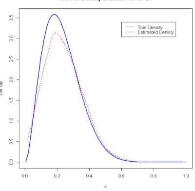
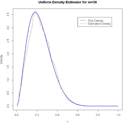
• Uniform Kernel Density Estimation
For this simulation, we consider the estimator:
Dn(x) =A· m n n X i=1 (1− |x−Xi|)m where A = 1
2 is the multiplicative factor to make the density estimator
consistent.
To estimate a uniform kernel, we assume X ∼ Beta(3,10) to be the true distribution with density function,
f(x) = x
2(1−x)9
B(3,10) ; 06x61 where B(3,10) = Γ(3)Γ(10)Γ(13) .
We show the estimate for different values of m (number of splits) in figures below:
m= 20 (fig.4.1) , 32 (fig.4.2), 39 (fig.4.3)
Figure 4.1: Uniform Kernel Density Estimate for m= 20
Figure 4.3: Uniform Kernel Density Estimate for m= 39
From the plots above, it can be observed that as the value ofmincreases, the estimated density gives a good fit of the true density as expected. However, for m > 39, the estimated density tends to exceed the bounds of the true density.
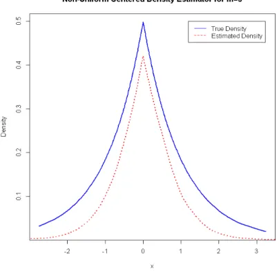
• Non-Uniform Kernel Density Estimation
To estimate a non-uniform kernel, we assume X ∼ Laplace(0,1) to be the true distribution with density function
g(x) = 1 2e
−|x|
, ∞< x <∞
and distribution function
G(x) = 1 2e x if x60 1− 1 2e −x if x>0
– Centred Non-Uniform Density Estimation
Here G(x)= 12 (i.e., symmetric G centred at x) and we consider the estimator: Dn(x) = A· m n n X i=1 (1− |1/2−G(x−Xi)|)m whereA= 1
2g(x) is multiplicative factor to make the estimator
consis-tent.
We show the estimate for different values of m (number of splits) in figures below:
m= 5 (fig.4.4), 8 (fig.4.5), 15 (fig.4.6).
Figure 4.5: Centred Non-Uniform Density Estimate for m= 8
From the plots above, it can be observed that the estimated density takes the curvature of the true density, but clearly, it does not provide a good fit asm increases.
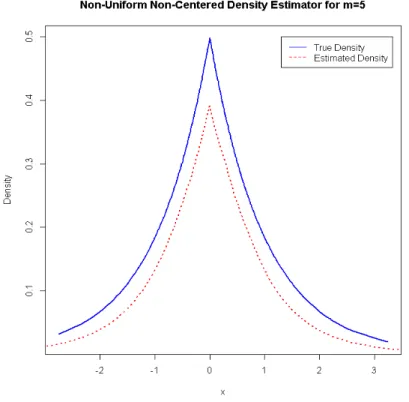
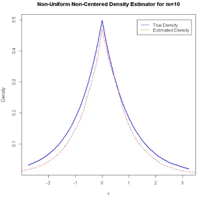
– Non-Centred Non-Uniform Density Estimation
Here, we consider the estimator:
Dn(x) = A· m n n X i=1 (1− |G(x)−G(Xi)|)m whereA= 1
2g(x) is multiplicative factor to make the estimator
consis-tent.
We show the estimate for different values of m (number of splits) in figures below:
m= 5 (fig.4.7), 10 (fig.4.8), 15 (fig.4.9)
Figure 4.8: Non-Centred Non-Uniform Density Estimate for m= 10
From the plots above, it can be observed that as we increase the value of
m, the estimated density gives a good fit of the true density as expected.
4.2
Regression Estimation
Consider the regression model
Yi =r(Xi) + 0.075i where, i ∼ N(0,1)
r(·) is the true distribution.
• Uniform Kernel Regression Estimation
Here, we consider the uniform regression estimator
Nn(x) = m n n X i=1 Yi(1− |x−Xi|)m
We assumeX ∼Beta(3,10) to be the true distribution with density function
f(x) = x
2(1−x)9
B(3,10) ; 06x61 where B(3,10) = Γ(3)Γ(10)Γ(13) .
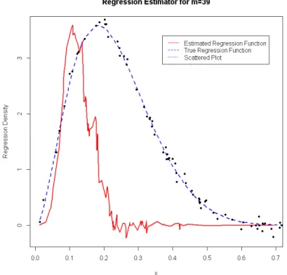
We show the estimate for different values of m (number of splits) in figures below:
Figure 4.10: Uniform Kernel Regression Estimate for m= 15
Figure 4.12: Uniform Kernel Regression Estimate for m= 39
From the plots above, it can be observed that the estimated regression ap-proaches the bounds of the true function. However, it does not provide a good fit.
• Non-Uniform Kernel Regression Estimation
To estimate a non-uniform kernel, we assume X ∼ Laplace(0,1) to be the true distribution with density function
g(x) = 1 2e
−|x|
, ∞< x <∞
and distribution function
G(x) = 1 2e x if x60 1− 1 2e −x if x>0
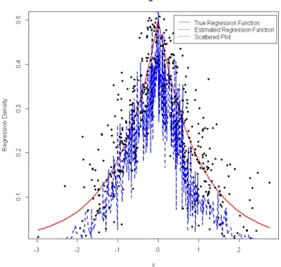
– Centred Non-Uniform Regression Estimation
Here G(x)= 12 (i.e., symmetric G centred at x) and we consider the regression estimator Nn(x) = m n n X i=1 Yi(1− |1/2−G(x−Xi)|)m
We show the estimate for different values of m (number of splits) in figures below:
m= 5 (fig.4.13), 20 (fig.4.14),n1/5 (fig.4.15)
Figure 4.14: Centred Non-Uniform Regression Estimate for m= 20
From the plots above, it can be observed that the estimated regression tries to fit the true function but there is a problem of over-fitting, as it tends to pass through every point. Hence, it does not provide a good fit.
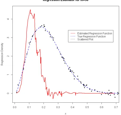
– Non-Centred Non-Uniform Regression Estimation
Here, we consider the regression estimator:
Nn(x) = m n n X i=1 Yi(1− |G(x)−G(Xi)|)m
We show the estimate for different values of m (number of splits) in figures below:
m= 2 (fig.4.16), 5 (fig.4.17), n1/3 (fig.4.18)
Figure 4.17: Non-Centred Non-Uniform Regression Estimate for m= 5
From the plots above, it can be observed that the estimated regression tries to fit the true function but there is a problem of over-fitting, as it tends to pass through every point. Hence, it does not provide a good fit.
5
Conclusion and Future work
In this paper, we sought to define a new estimators for both density and regression kernels. Scornet (Scornet,2016b) had an expression for kernelKkuf which only had simple representation for level k = 1,2. However, when levels were greater than 2, the expression became extremely complicated to compute. We used different partitioning scheme to find the general expression for the both uniform and non-uniform kernels and from that we had a density and regression estimators.
We studied the consistency and asymptotic normality of the estimators and finally used simulation to evaluate the performance of the estimators.
In Chapter 4, we realized that the new density estimators provide good fit to the true function but depends heavily on m, the number of splits, whiles the new regression estimators did not provide a good fit to the true function.
In future, research can be done on:
• developing procedure for the optimal data-based choice of m, and • extending the results to directional data.
• investigating if theorem 3.2 holds for non-absolute continuous distribution
References
Arlot, S., & Genuer, R. (2014). Analysis of purely random forests bias. arXiv preprint arXiv:1407.3939.
Biau, G., Devroye, L., & Lugosi, G. (2008). Consistency of random forests and other averaging classifiers. Journal of Machine Learning Research, 9(Sep), 2015–2033.
Biau, G., & Scornet, E. (2016). A random forest guided tour. Test, 25(2), 197–227.
Breiman, L. (2000). Some infinity theory for predictor ensembles (Tech. Rep.). Technical Report 579, Statistics Dept. UCB.
Denil, M., Matheson, D., & Freitas, N. (2013). Consistency of online random forests. In International conference on machine learning (pp. 1256–1264). Mentch, L., & Hooker, G. (2016). Quantifying uncertainty in random forests via
confidence intervals and hypothesis tests. The Journal of Machine Learning Research, 17(1), 841–881.
Nadaraya, E. A. (1964). On estimating regression. Theory of Probability & Its Applications,9(1), 141–142.
Scornet, E. (2016a). On the asymptotics of random forests.Journal of Multivariate Analysis,146, 72–83.
Scornet, E. (2016b). Random forests and kernel methods. IEEE Transactions on Information Theory, 62(3), 1485–1500.
Wager, S. (2014). Asymptotic theory for random forests. arXiv preprint arXiv:1405.0352.
Watson, G. S. (1964). Smooth regression analysis. Sankhy¯a: The Indian Journal of Statistics, Series A, 359–372.
A
R Codes
A.1
Uniform density estimator
• For m=20 set.seed(16) n=500 x=sort(runif(n)) #true den. fx= dbeta(x,3,10) rx=function(v,m,xi){ b=beta(3,10) a = rep(0,length(v)) for(i in 1:(length(v))){ a[i]=(m/(2*n))*sum((1-abs(v[i]-xi))^m) } return(a) } xi = rbeta(n,3,10) v = sort(rbeta(n,3,10))vx = rx(v,m=20,xi)
plot(x,fx,type = ’l’,col= "blue",lwd=2,ylab = "Density",
main = "Uniform Density Estimator for m=20")
lines(v,vx,col="Red", lty=3,lwd=2)
legend(0.6,3.4,legend = c("True Density","Estimated Density"),
col = c(’Blue’,"red"),lty=1:2) • For m=32 set.seed(16) n=500 x=sort(runif(n)) #true den. fx= dbeta(x,3,10) rx=function(v,m,xi){ b=beta(3,10) a = rep(0,length(v)) for(i in 1:(length(v))){ a[i]=(m/(2*n))*sum((1-abs(v[i]-xi))^m) } return(a) } xi = rbeta(n,3,10) v = sort(rbeta(n,3,10)) vx = rx(v,m=32,xi)
plot(x,fx,type = ’l’,col= "blue",lwd=2,ylab = "Density",
main = "Uniform Density Estimator for m=32")
lines(v,vx,col="Red", lty=3,lwd=2)
legend(0.6,3.4,legend = c("True Density","Estimated Density"),
col = c(’Blue’,"red"),lty=1:2) • For m=39 set.seed(16) n=500 x=sort(runif(n)) #true den. fx= dbeta(x,3,10) rx=function(v,m,xi){ b=beta(3,10) a = rep(0,length(v)) for(i in 1:(length(v))){ a[i]=(m/(2*n))*sum((1-abs(v[i]-xi))^m) } return(a) } xi = rbeta(n,3,10) v = sort(rbeta(n,3,10)) vx = rx(v,m=39,xi)
plot(x,fx,type = ’l’,col= "blue",lwd=2,ylab = "Density",
main = "Uniform Density Estimator for m=39")
lines(v,vx,col="Red", lty=3,lwd=2)
legend(0.6,3.4,legend = c("True Density","Estimated Density"),
col = c(’Blue’,"red"),lty=1:2)
A.2
Non-Uniform Density Estimator
A.2.1
Centered Density Estimator
• m=5 set.seed(16) n=500 library(rmutil) #true density x=sort(rnorm(n)) gx= dlaplace(x) rx=function(v,m,xi){ a = rep(0,length(v)) for(i in 1:(length(v))){ a[i]=(dlaplace(v[i])/2)*(m/n)*sum((1-abs(0.5-pnorm(v[i]-xi)))^m) } return(a) }
xi = rnorm(n)
v = sort(rlaplace(n))
vx = rx(v,m=5,xi)
plot(x,gx,type = ’l’,col= "blue",lwd=2,ylab = "Density",
main = "Non-Uniform Centered Density Estimator for m=5")
lines(v,vx,col="Red", lty=3,lwd=2)
legend(1.2,0.5,legend = c("True Density","Estimated Density"),
col = c(’Blue’,"red"),lty=1:2) • m=8 set.seed(16) n=500 library(rmutil) #true density x=sort(rnorm(n)) gx= dlaplace(x) rx=function(v,m,xi){ a = rep(0,length(v)) for(i in 1:(length(v))){ a[i]=(dlaplace(v[i])/2)*(m/n)*sum((1-abs(0.5-pnorm(v[i]-xi)))^m) } return(a) }
xi = rnorm(n)
v = sort(rlaplace(n))
vx = rx(v,m=8,xi)
plot(x,gx,type = ’l’,col= "blue",lwd=2,ylab = "Density",
main = "Non-Uniform Centered Density Estimator for m=8")
lines(v,vx,col="Red", lty=3,lwd=2)
legend(1.2,0.5,legend = c("True Density","Estimated Density"),
col = c(’Blue’,"red"),lty=1:2) • m= 15 set.seed(16) n=500 library(rmutil) #true density x=sort(rnorm(n)) gx= dlaplace(x) rx=function(v,m,xi){ a = rep(0,length(v)) for(i in 1:(length(v))){ a[i]=(dlaplace(v[i])/2)*(m/n)*sum((1-abs(0.5-pnorm(v[i]-xi)))^m) } return(a) }
xi = rnorm(n)
v = sort(rlaplace(n))
vx = rx(v,m=15,xi)
plot(x,gx,type = ’l’,col= "blue",lwd=2,ylab = "Density",
main = "Non-Uniform Centered Density Estimator for m=15")
lines(v,vx,col="Red", lty=3,lwd=2)
legend(1.2,0.5,legend = c("True Density","Estimated Density"),
col = c(’Blue’,"red"),lty=1:2)
A.2.2
Non-Centered Density Estimator
• m= 5 set.seed(16) n=500 library(rmutil) #true density x=sort(rnorm(n)) gx= dlaplace(x) rx=function(v,m,xi){ a = rep(0,length(v)) for(i in 1:(length(v))){ a[i]=(dlaplace(v[i])/2)*(m/n)*sum((1-abs(plaplace(v[i])-pnorm(xi)))^m) } return(a) }
xi = rnorm(n)
v = sort(rlaplace(n))
vx = rx(v,m=5,xi)
plot(x,gx,type = ’l’,col= "blue",lwd=2,ylab = "Density",
main = "Non-Uniform Non-Centered Density Estimator for m=5")
lines(v,vx,col="Red", lty=3,lwd=2)
legend(1.3,0.5,legend = c("True Density","Estimated Density"),
col = c(’Blue’,"red"),lty=1:2) • m= 10 set.seed(16) n=500 library(rmutil) #true density x=sort(rnorm(n)) gx= dlaplace(x) rx=function(v,m,xi){ a = rep(0,length(v)) for(i in 1:(length(v))){ a[i]=(dlaplace(v[i])/2)*(m/n)*sum((1-abs(plaplace(v[i])-pnorm(xi)))^m) } return(a) }
xi = rnorm(n)
v = sort(rlaplace(n))
vx = rx(v,m=10,xi)
plot(x,gx,type = ’l’,col= "blue",lwd=2,ylab = "Density",
main = "Non-Uniform Non-Centered Density Estimator for m=10")
lines(v,vx,col="Red", lty=3,lwd=2)
legend(1.3,0.5,legend = c("True Density","Estimated Density"),
col = c(’Blue’,"red"),lty=1:2) • m= 15 set.seed(16) n=500 library(rmutil) #true density x=sort(rnorm(n)) gx= dlaplace(x) rx=function(v,m,xi){ a = rep(0,length(v)) for(i in 1:(length(v))){ a[i]=(dlaplace(v[i])/2)*(m/n)*sum((1-abs(plaplace(v[i])-pnorm(xi)))^m) } return(a) } xi = rnorm(n)
v = sort(rlaplace(n))
vx = rx(v,m=15,xi)
plot(x,gx,type = ’l’,col= "blue",lwd=2,ylab = "Density",
main = "Non-Uniform Non-Centered Density Estimator for m=15")
lines(v,vx,col="Red", lty=3,lwd=2)
legend(1.3,0.5,legend = c("True Density","Estimated Density"),
col = c(’Blue’,"red"),lty=1:2)
A.3
Uniform Regression Estimator
• m= 15 set.seed(1) n=500 x=sort(runif(n)) #true density fx= dbeta(x,3,10) x1=sort(rbeta(n,3,10)) yi=fx+(0.075)*rnorm(n) rx=function(y,v,m,xi){ #b=beta(3,10) a = rep(0,length(v)) for(i in 1:(length(v))){ a[i]=(15-(1/(b*n)))/n)*sum(y[i]*(1-abs(v[i]-xi))^m) } return(a) }xi = rbeta(n,3,10)
v = sort(rbeta(n,3,10))
vx = rx(y=yi,v,m=15,xi)
plot(v,vx,type = "l", col=’red’, lwd=2,xlab="x", ylab =
’Regression Density’,
main = "Regression Estimator for m=15") #estimated regression
lines(x,fx, lwd=2, col=’Blue’, lty=2) #True regrssion function
points(x,yi, col=’black’, pch=20) #Scattered
legend(0.37,3.4,legend = c("Estimated Regression Function",
"True Regression Function"
,"Scattered Plot"),col = c(’red’,"blue","black"),lty=c(1,2,3))
• m= 30 set.seed(1) n=100 x=sort(runif(n)) #true density fx= dbeta(x,3,10) x1=sort(rbeta(n,3,10)) yi=fx+(0.075)*rnorm(n) rx=function(y,v,m,xi){ b=beta(3,10) a = rep(0,length(v)) for(i in 1:(length(v))){ a[i]=((15-(1/(b*n)))/n)*sum(y[i]*(1-abs(v[i]-xi))^m)
} return(a) } xi = rbeta(n,3,10) v = sort(rbeta(n,3,10)) vx = rx(y=yi,v,m=30,xi)
plot(v,vx,type = "l", col=’red’, lwd=2, ylab = ’Regression Density’,
main = "Regression Estimator for m=30") #estimated regression
lines(x,fx, lwd=2, col=’Blue’, lty=2) #True regression function
points(x,yi, col=’black’, pch=20) #Scattered plot
legend(0.37,3.4,legend = c("Estimated Regression Function",
"True Regression Function","Scattered Plot"),
col = c(’red’,"blue","black"),lty=1:2:3) • m=39 set.seed(1) n=100 x=sort(runif(n)) #true density fx= dbeta(x,3,10) x1=sort(rbeta(n,3,10)) yi=fx+(0.075)*rnorm(n) rx=function(y,v,m,xi){ b=beta(3,10) a = rep(0,length(v)) for(i in 1:(length(v))){
a[i]=((15-(1/(b*n)))/n)*sum(y[i]*(1-abs(v[i]-xi))^m) } return(a) } xi = rbeta(n,3,10) v = sort(rbeta(n,3,10)) vx = rx(y=yi,v,m=39,xi)
plot(v,vx,type = "l", col=’red’, lwd=2, ylab = ’Regression Density’,
main = "Regression Estimator for m=39") #estimated regression
lines(x,fx, lwd=2, col=’Blue’, lty=2) #True regression function
points(x,yi, col=’black’, pch=20) #Scattered plot
legend(0.37,3.4,legend = c("Estimated Regression Function",
"True Regression Function","Scattered Plot"),
col = c(’red’,"blue","black"),lty=1:2:3)
A.4
Non-Uniform Regression Estimator
A.4.1
Centered Regression Estimator
• m=5 set.seed(7) n=500 x=sort(rnorm(n)) #true density fx= dlaplace(x) yi=fx+(0.075)*rnorm(n)
rx=function(y,v,m,xi){ a = rep(0,length(v)) for(i in 1:(length(v))){ a[i]=(m/(2*n))*sum(y[i]*(1-abs(0.5-pnorm(v[i]-xi)))^m) } return(a) } xi = rnorm(n) v = sort(rlaplace(n)) vx = rx(y=yi,v,m=5,xi)
plot(x,fx,type = "l", col=’red’, lwd=2,xlab="x", ylab =
’Regression Density’,
main = "Non-Uniform Centered Regression Estimator for m=5")
#True regression
lines(v,vx, lwd=2, col=’Blue’, lty=2) #Estimated regression function
points(x,yi, col=’black’, pch=20) #Scattered
legend(0.383,0.51,legend = c("True Regression Function",
"Estimated Regression Function","Scattered Plot"),
col = c(’red’,"blue","black"),lty=c(1,2,3))
• m=20
set.seed(7)
n=500
#true density fx= dlaplace(x) yi=fx+(0.075)*rnorm(n) rx=function(y,v,m,xi){ a = rep(0,length(v)) for(i in 1:(length(v))){ a[i]=(m/(2*n))*sum(y[i]*(1-abs(0.5-pnorm(v[i]-xi)))^m) } return(a) } xi = rnorm(n) v = sort(rlaplace(n)) vx = rx(y=yi,v,m=20,xi)
plot(x,fx,type = "l", col=’red’, lwd=2,xlab="x", ylab =
’Regression Density’,
main = "Non-Uniform Centered Regression Estimator for m=20")
#True regression
lines(v,vx, lwd=2, col=’Blue’, lty=2) #Estimated regression function
points(x,yi, col=’black’, pch=20) #Scattered
legend(0.383,0.51,legend = c("True Regression Function",
"Estimated Regression Function","Scattered Plot"),
col = c(’red’,"blue","black"),lty=c(1,2,3))
library(rmutil) set.seed(7) n=500 x=sort(rnorm(n)) #true density fx= dlaplace(x) # x1=sort(rbeta(n,3,10)) yi=fx+(0.075)*rnorm(n) rx=function(y,v,m,xi){ a = rep(0,length(v)) for(i in 1:(length(v))){ a[i]=(m/(2*n))*sum(y[i]*(1-abs(0.5-pnorm(v[i]-xi)))^m) } return(a) } xi = rnorm(n) v = sort(rlaplace(n)) vx = rx(y=yi,v,m=(n^(1/5)),xi)
plot(x,fx,type = "l", col=’red’, lwd=2,xlab="x", ylab =
’Regression Density’,
main = "Non-Uniform Centered Regression Estimator for m=n^1/5")
#True regression
lines(v,vx, lwd=2, col=’Blue’, lty=2) #Estimated regrssion function
legend(0.28,0.51,legend = c("True Regression Function",
"Estimated Regression Function","Scattered Plot"),
col = c(’red’,"blue","black"),lty=c(1,2,3))
A.4.2
Non-Centered Regression Estimator
• m=2 set.seed(7) n=500 x=sort(rnorm(n)) #true density fx= dlaplace(x) yi=fx+(0.075)*rnorm(n) rx=function(y,v,m,xi){ a = rep(0,length(v)) for(i in 1:(length(v))){ a[i]=(m/(1.8*n))*sum(y[i]*(1-abs(plaplace(v[i])-pnorm(xi)))^m) } return(a) } xi = rnorm(n) v = sort(rlaplace(n)) vx = rx(y=yi,v,m=2,xi)
’Regression Density’,
main = "Non-Uniform Non-Centered Regression Estimator for m=2")
#True regression
lines(v,vx, lwd=2, col=’Blue’, lty=2) #estimated regression function
points(x,yi, col=’black’, pch=20) #Scattered
legend(0.4,0.51,legend = c("True Regression Function",
"Estimated Regression Function","Scattered Plot"),
col =c(’red’,"blue","black"),lty=c(1,2,3)) • m=5 set.seed(7) n=500 x=sort(rnorm(n)) #true density fx= dlaplace(x) yi=fx+(0.075)*rnorm(n) rx=function(y,v,m,xi){ a = rep(0,length(v)) for(i in 1:(length(v))){ a[i]=(m/(1.8*n))*sum(y[i]*(1-abs(plaplace(v[i])-pnorm(xi)))^m) } return(a) } xi = rnorm(n) v = sort(rlaplace(n)) vx = rx(y=yi,v,m=5,xi)
plot(x,fx,type = "l", col=’red’, lwd=2,xlab="x", ylab =
’Regression Density’,
main = "Non-Uniform Non-Centered Regression Estimator for m=5")
#True regression
lines(v,vx, lwd=2, col=’Blue’, lty=2) #estimated regression function
points(x,yi, col=’black’, pch=20) #Scattered
legend(0.4,0.51,legend = c("True Regression Function",
"Estimated Regression Function","Scattered Plot"),
col = c(’red’,"blue","black"),lty=c(1,2,3)) • m=n1/3 set.seed(7) n=500 x=sort(rnorm(n)) #true density fx= dlaplace(x) yi=fx+(0.075)*rnorm(n) rx=function(y,v,m,xi){ a = rep(0,length(v)) for(i in 1:(length(v))){ a[i]=(m/(2*n))*sum(y[i]*(1-abs(plaplace(v[i])-pnorm(xi)))^m) } return(a) }