Durham E-Theses
Finite mixture models: visualisation, localised
regression, and prediction
QARMALAH, NAJLA,MOHAMMED,A
How to cite:
QARMALAH, NAJLA,MOHAMMED,A (2018) Finite mixture models: visualisation, localised regression, and prediction, Durham theses, Durham University. Available at Durham E-Theses Online:
http://etheses.dur.ac.uk/12486/
Use policy
The full-text may be used and/or reproduced, and given to third parties in any format or medium, without prior permission or charge, for personal research or study, educational, or not-for-prot purposes provided that:
• a full bibliographic reference is made to the original source
• alinkis made to the metadata record in Durham E-Theses
• the full-text is not changed in any way
The full-text must not be sold in any format or medium without the formal permission of the copyright holders. Please consult thefull Durham E-Theses policyfor further details.
Academic Support Oce, Durham University, University Oce, Old Elvet, Durham DH1 3HP e-mail: e-theses.admin@dur.ac.uk Tel: +44 0191 334 6107
http://etheses.dur.ac.uk
Finite mixture models:
visualisation, localised regression,
and prediction
Najla Mohammed Ashiq Qarmalah
A thesis presented for the degree of
Doctor of Philosophy
Department of Mathematical Sciences
Durham University
United Kingdom
February 2018
Dedicated to
my parents
whose affection, love,
encouragement and prayers of day
and night make me able to get such
Finite mixture models: visualisation,
localised regression, and prediction
Najla Mohammed Ashiq Qarmalah
Submitted for the degree of Doctor of Philosophy
February 2018
Abstract: Initially, this thesis introduces a new graphical tool, that can be used to summarise data possessing a mixture structure. Computation of the required summary statistics makes use of posterior probabilities of class membership obtained from a fitted mixture model. In this context, both real and simulated data are used to highlight the usefulness of the tool for the visualisation of mixture data in comparison to the use of a traditional boxplot.
This thesis uses localised mixture models to produce predictions from time series data. Estimation method used in these models is achieved using a kernel-weighted version of an EM–algorithm: exponential kernels with different bandwidths are used as weight functions. By modelling a mixture of local regressions at a target time point, but using different bandwidths, an informative estimated mixture probabilities can be gained relating to the amount of information available in the data set. This information is given a scale of resolution, that corresponds to each bandwidth. Nadaraya-Watson and local linear estimators are used to carry out localised estimation. For prediction at a future time point, a new methodology of bandwidth selection and adequate methods are proposed for each local method, and then compared to competing forecasting routines. A simulation study is executed to assess the performance of this model for prediction. Finally, double-localised mixture models are presented, that can be used to improve predictions for a variable time series using additional information provided by other time series. Estimation for these models is achieved using a double-kernel-weighted
Abstract iv
version of the EM–algorithm, employing exponential kernels with different horizontal bandwidths and normal kernels with different vertical bandwidths, that are focused around a target observation at a given time point. Nadaraya-Watson and local linear estimators are used to carry out the double-localised estimation. For prediction at a future time point, different approaches are considered for each local method, and are compared to competing forecasting routines. Real data is used to investigate the performance of the localised and double-localised mixture models for prediction. The data used predominately in this thesis is taken from the International Energy Agency (IEA).
Declaration
The work in this thesis is based on research carried out in the Department of Mathe-matical Sciences, Durham University, United Kingdom. No part of this thesis has been submitted elsewhere for any other degree or qualification and it is all my own work unless referenced to the contrary in the text.
Copyright c February 2018 by Najla Mohammed Ashiq Qarmalah.
“The copyright of this thesis rests with the author. No quotations from it should be published without the author’s prior written consent and information derived from it should be acknowledged.”
Acknowledgements
I would like to express my sincere gratitude to Allah for the countless blessings he has bestowed on me, both in general and particularly during my work on this thesis. My appreciation and special thanks go to my supervisors, Prof. Frank Coolen and Dr. Jochen Einbeck, for their unlimited support, expert advice and guidance in all the time of research and writing of this thesis. I appreciate their high standards, ability, and knowledge of research methodology. It is really hard to find the words to express my gratitude and appreciation for them.
I am immensely grateful to my parents for their faith, support, and constant encour-agement. I thank my parents for teaching me to believe in Allah, in myself, and in my dream. I hope my parents are proud of this thesis.
I want to acknowledge my closest supporters, my brothers and sisters, for their confi-dence and constant encouragement, and my family and friends, who have been a great source of motivation through all these years.
I am also grateful to my country, Saudi Arabia, represented by King Salman, Saudi Arabian Cultural Bureau in London, Ministry of Education and Princess Norah bint Abdul Rahman University in Riyadh for granting me the scholarship and providing me with this great opportunity for completing my studies in the UK and so enabling me to fulfil my ambition.
Many thanks to Durham University for offering such an enjoyable academic atmosphere and for the facilities, that have enabled me to study smoothly.
My final thanks go to everyone who has assisted me, stood by me or contributed to my educational progress in any way.
Contents
Abstract iii 1 Introduction 1 1.1 Overview . . . 1 1.2 Local modelling . . . 3 1.2.1 Nadaraya-Watson estimator . . . 51.2.2 Local polynomial estimator . . . 6
1.3 Local likelihood estimation . . . 9
1.4 Mixture models . . . 11
1.4.1 Mixture models estimation . . . 13
1.4.2 Choosing the number of components . . . 16
1.5 Prediction . . . 18
1.6 Outline of thesis . . . 20
2 Visualisation of mixture data 22 2.1 Introduction . . . 22
2.2 Computational elements of K–boxplots . . . 26
2.2.1 Posterior probabilities . . . 26
2.2.2 Weighted quartiles . . . 28
2.3 Examples . . . 29 vii
Contents viii
2.3.1 Example 1: energy use data . . . 29
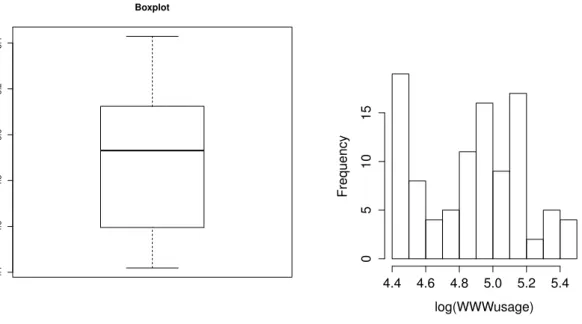
2.3.2 Example 2: internet users data . . . 34
2.3.3 Simulation . . . 36
2.4 Conclusions . . . 38
3 Localised mixture models for prediction 41 3.1 Introduction . . . 41
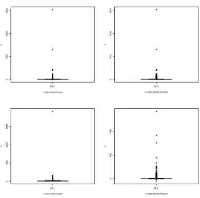
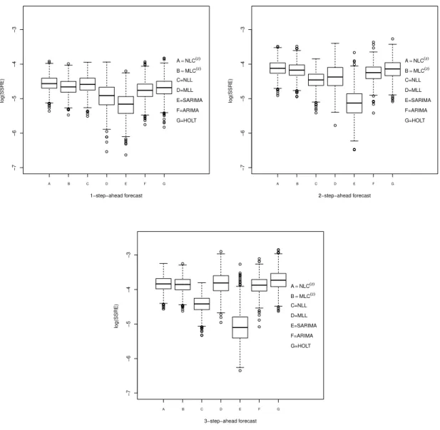
3.2 Mixture models using local constant kernel estimators (MLC) . . . 42
3.3 Mixture models using local linear kernel estimators (MLL) . . . 46
3.4 Identifiability . . . 48 3.5 Model selection . . . 52 3.6 Forecasting . . . 53 3.7 Simulation methodology . . . 54 3.8 Simulation study . . . 57 3.8.1 Example 1 . . . 57 3.8.2 Example 2 . . . 66 3.9 Applications . . . 72 3.10 Conclusions . . . 79
4 Double-localised mixture models for prediction 81 4.1 Introduction . . . 81
4.1.1 Motivation . . . 83
4.2 Mixture models using local constant kernel estimators and vertical ker-nels (MLCV) . . . 86
4.3 Mixture models using local linear kernel estimators and vertical kernels (MLLV) . . . 89
Contents ix
4.5 Forecasting . . . 93
4.5.1 Forecasting using localised mixture models for multi-valued re-gression data . . . 93
4.5.2 Forecasting using double localised mixture models . . . 94
4.6 Applications . . . 95
4.7 Conclusions . . . 104
5 Conclusions and future research 107 5.1 Conclusions . . . 107
5.2 Future research . . . 109
A Brief guide to notation 118
B 119
C 120
Chapter 1
Introduction
1.1
Overview
The use of finite mixture models is a source of much debate mainly, because of the flexibility of the models across a wide variety of random phenomena, and the increase in available computing power. Finite mixture models have been successfully applied in many fields. For example, according to Mclachlan and Peel [62], applications of finite mixture models have been used in astronomy, biology, medicine, psychiatry, genetics, economics, engineering, and marketing, among many other fields in the biological, physical, and social sciences. In addition, finite mixture models have applications including cluster and latent class analyses, discriminant analysis, image analysis and survival analysis [62].
The use of finite mixture models has increased considerably over the past decade and the use of these models has continued to receive increasing attention in the years, both from a practical and theoretical point of view. In the 1990s, finite mixture models were extended by mixing standard linear regression models as well as generalised linear models [90]. Lindsay [57] discusses the non-parametric and semi-parametric maximum likelihood estimation used in mixture models, while Mclachlan and Peel [62] discuss the major problems relating to mixture models. Some issues discussed by both include identifiability problems, the EM–algorithm, the properties of the maximum likelihood estimators so obtained, and the assessment of the number of components used in the mixture.
1.1. Overview 2
One of the most popular mixture models is the mixture of Gaussian distributions due to its applications in various fields. This model is classed as the first mixture model as used by Karl Pearson [65]. Pearson fits a mixture of two Gaussian probability density functions with different means and variances. In fact, Gaussian mixture models are used in the investigation of the performances of certain estimators as departures from normality [62]. Consequently, Gaussian mixture models have been used in the devel-opment of robust estimators [62]. For example, under the contaminated normal family as outlined by Tukey [81], the density of an observation is taken to be a mixture of two univariate Gaussian densities with the same means but where the second component has a greater variance than the first.
The initial focus of this thesis is to develop a new graphical tool, that can be used to visualise Gaussian mixture data. This new graphical tool can provide additional information to the data analyst, where traditional plots cannot. Notably, this new plot can be applied to data, which belongs to any mixture of density distributions. This idea will be discussed in more detail in Chapter 2. In addition, a mixture of local regression models is developed for prediction from time series using two approaches. In the first approach, a mixture of local regression model is developed for prediction using past information from a target time series. This will be discussed in more detail in Chapter 3. Moreover, in the second approach, additional information is used from other time series, that is relevant to the target time series, in order to stabilise the prediction of the target time series in comparison with other time series models. This problem will be investigated in Chapter 4.
This first chapter will review local modelling as represented in local polynomial re-gression, and local likelihood methods. Previous research about mixture models used unknown distributional shapes of data will be presented and one of the most impor-tant classes of mixture models, a mixture of non-parametric regression models, will be discussed. In addition, popular estimation methods used in mixture models, such as the EM–algorithm and its application on mixtures of non-parametric regression mod-els will be explained in more detail. This thesis examines the EM–algorithm in more detail in Chapter 2 and more advanced versions of the EM–algorithm in Chapters 3 and 4. In addition, several methodologies used for prediction are reviewed such as the
1.2. Local modelling 3
ARIMA and Holt models, which can be compared with the newly proposed methods for prediction as outlined in Chapters 3 and 4. This context is used to develop the new graphical tool for visualising mixture models and prediction from time series using new methodologies based on mixtures and local regression models.
1.2
Local modelling
Regression is one of the most commonly used statistical methods, simply because it can be applied across many research fields, including: econometrics, social science, medicine, and psychology. Linear regression is a classical and widely technique used, in order to study the relationship between variables and to fit a line through data. A simple linear regression model for given pairs of data such as (xi, yi), i= 1, . . . , ntakes
the form as follows:
y=β0+β1x+ (1.2.1)
where β0 and β1 are the parameters, that represent the intercept and slope of the
model, respectively. If the observed data has a linear trend, then the model (1.2.1) can be said to fit the data well, and parameters can be estimated using the least squares method. However, when the observed data takes a more complex shape, and cannot be converted into a linear relationship using transformation, then linear regression may not be an appropriate method to use. Consequently, a non-parametric regression model is considered to be a more useful technique for relaxing linearity assumption, and to avoid the restrictive assumptions relating to the functional form of the regression function [23]. Indeed, non-parametric regression belongs to a class of regression techniques whereby, according to Wand and Jones [85], the model is shaped completely based on the data. The non-parametric method is particularly useful to use when a parametric model becomes too restrictive.
There are several different non-parametric regression techniques, that can be used, and these can, generally, be split into the categories of spline-based and local methods [23]. Thus, instead of solving a parametric problem as demonstrated in the model (1.2.1), we can solve many linear regression problems using only two parameters β0(x) and
1.2. Local modelling 4
neighbourhood, known as a bandwidth or a smoothing parameter, then the local linear regression model can be defined as follows:
yi =β0(x) +β1(x)xi+i, x−h≤xi ≤x+h
where β0(x) andβ1(x) are the parameters that depend on x.
A general non-parametric regression model can be written as:
yi =m(xi1, xi2, . . . , xiq) +εi
wherem(·) is known as the regression function, whilexi1, xi2, . . . , xiqareqpredictors for
the i-th of n observations. The errors εi are assumed to be independently distributed,
with a mean of 0 and a constant variance of σ2 [26]. However, most methods of non-parametric regression implicitly assume, that m(·) is a smooth continuous function [26]. One important instance of non-parametric regression is known as non-parametric simple regression, where there is only one predictor [23]:
yi =m(xi) +εi (1.2.2)
This type of non-parametric regression is often called ‘scatterplot smoothing’ , because it traces a smooth curve through a scatterplot of y againstx [26]
An important issue, that must be settled before using a local fitting technique is deter-mining the ‘local neighbourhood’ or the window, which is commonly described using the kernel functionW and the bandwidth parameter h[23]. The kernel function W is a weight function, that it weighs observations close to the target point more heavily and assigns a weight of 0 to far away observations [39]. According to Härdle et al. [39], for all the other kernel methods, the bandwidthhdetermines the degree of smoothness of the regression function estimation ˆm(·) by controlling the weights of the observation points used in the local neighbourhood. The larger the local neighbourhood, then the smoother the estimated regression function is. The bandwidth h can be chosen to be constant or to depend on the location [21]. The choice of the bandwidth h is more crucial than the kernel function, because it determines the complexity of a model. For example, when a bandwidth h = 0, this results in interpolating the data, which leads to the most complex model. On the other hand, when htends to ∞, the data is fitted
1.2. Local modelling 5
globally, which is the simplest model. As a result, a bandwidth governs the complexity of the model [21]. The choice of kernel function does not mainly affect the perfor-mance of the resulting estimation in non-parametric regression, both theoretically and empirically [21]. Wand and Jones [85] discuss the effect of the kernel function on non-parametric smoothing estimation based on asymptotic mean integrated squared error (AMISE) criterion. The result suggests that most unimodel kernel functions perform about the same as each other, see for more detail [59].
Local fitting is indeed a particularly useful technique to use in non-parametric estima-tion [79]. This local modelling approach aims to relax the global linearity assumpestima-tion through the local linear model, which results in a new objective function called the local maximum likelihood function [23]. In order to fit the regression function m(x) in the model (1.2.2) at a particular point of x0 locally, there are many ways, that can
be used to evaluate the estimator of m(x), where the data set can fit the smoother ˆ
y= ˆm(x).
1.2.1
Nadaraya-Watson estimator
Nadaraya [64] and Watson [88] proposed a kernel regression estimator, usually referred to as the Nadaraya-Watson estimator, or local constant regression estimator. It belongs to a class of kernel regression estimators, that correspond to a local constant least squares fit. The Nadaraya-Watson estimator weighs the local average of the response variables yi. In the Nadaraya-Watson estimator, when h → 0, then ˆm(xi) converges
to yi at an observation xi. As discussed in Section 1.2, the behaviour is different
for h → ∞, where an infinitely large h makes all weights equal, and local modelling becomes global modelling [39]. The main difference between parametric and non-parametric modelling is that for the former the bandwidth h is always infinite, but different parametric families of models are used. In non-parametric modelling, as in local modelling, several different bandwidths used need to be considered, so that the resulting curve articulates a given data set [23].
In definition, W is the real-value kernel function for assigning weights, and h is the bandwidth, a non-negative number, that controls the size of the local neighbourhood.
1.2. Local modelling 6
The Nadaraya-Watson kernel regression estimator can be represented as: ˆ m(x) = Pn i=1Wh(xi−x)yi Pn i=1Wh(xi−x)
where Wh(·) = W(·/h)/h [23]. The function W is usually taken to be a symmetric
probability density, because it yields smaller mean integrated squared error (MISE). The MISE can be presented as follows [73]
MISE(x) =
Z
MSE(u)W(u)du
where W(·) is a weight function where W(·)≥0 and MSE(·) is a mean squared error which is defined as follows
MSE(x) =Eh{mˆ(x)−m(x)}2i
See for a detailed discussion of symmetric kernel function [14]. For example, the Gaus-sian kernel is widely used for non-parametric smoothing. It is defined by the GausGaus-sian probability density function as follows:
W(x) = √1
2πexp
−x2/2 (1.2.3)
The kernel function based on a Gaussian probability density function, as defined in Equation (1.2.3) will be used later in Chapter 4.
1.2.2
Local polynomial estimator
In local polynomial regression, we first apply a Taylor expansion to m(x) in a neigh-bourhood of x0 as follows:
m(x)≈m(0)(x0)/0! +m(1)(x0)/1!(x−x0) +. . .+m(p)(x0)/p!(x−x0)p =xTβ (1.2.4)
wherex={1, x−x0, . . . ,(x−x0)p}
T
,β= (β0, . . . , βp)T such thatβj =m(j)(x0)/j!, j =
0, . . . , p and p is the degree of the polynomial. The points close to x0 will have more
influence on the estimate ofm(x0), while the points furthest fromx0 will have the least
influence [23]. A kernel function Wh puts more weight on the points near x0, and less
1.2. Local modelling 7
Method Bias Variance
Nadaraya-Watson d2 dx2m(x) + 2dxdm(x)dxdf(x) f(x) ! bn Vn Local linear dxd22m(x)bn Vn bn= 1 2h 2R∞ −∞u2W(u)du, Vn= σ 2(x) f(x)nh R∞ −∞W2(u)du
Table 1.1: Asymptotic biases and variances
polynomial regression can be minimised with respect to β0, β1. . . , and βp as follows: n X i=1 {yi−β0−β1(xi−x0). . .−βp(xi−x0)p} 2 Wh(xi−x0) (1.2.5)
The kernel function Wh controls the weights of the points at different locations. The
resulting estimator is called the local polynomial regression estimator. For convenience, this can be denoted as follows:
W = diag{Wh(x1−x0), . . . , Wh(xn−x0)}, X = xT 1 .. . xT n = 1, x1−x0 . . . , (x1−x0)p .. . ... . . . , ... 1, xn−x0 . . . , (xn−x0)p
Then, the solution to the locally weighted least squares problem as presented in Equa-tion (1.2.5) as follows:
ˆ
β = (XTW X)−1XTW y
ˆ
m(x0) = eT1 ×βˆ
where y = (y1, . . . , yn)T, and e1 = (1,0, . . . ,0)T is a 1×(p+ 1) vector with the first
entry being 1 and the others 0. Furthermore, we can obtain an estimate of the q-th (q < p) derivative of m(x) is as follows:
ˆ
m(q)(x0) =q!eTq+1βˆ
where eq+1 is a 1×(p+ 1) vector with (q+ 1)-th entry one and others 0 [23].
The Nadaraya-Watson estimator or local constant estimator is a special case of poly-nomial regression estimator when p= 0. When p= 1, the local polynomial regression estimator is known as a local linear estimator [23]. The asymptotic bias and variance
1.2. Local modelling 8
properties for a random design of the two estimators are summarised in Table 1.1 [23]. If we look at Table 1.1, we can see that a local linear estimator produces a more con-cise form of asymptotic bias than the Nadaraya-Watson estimator, but the asymptotic variances are the same. In addition, the local linear estimator offers several useful prop-erties, such as automatic correction of boundary effects [13, 22, 59], design adaptivity, and best asymptotic efficiency using the minimax criteria [20]. Fan and Gijbels [23] offer a comprehensive account of local polynomial regression. In general, asymptotic and boundary bias correction advantages correspond to the local linear p= 1 and the local cubic p = 3 estimators are obtained. In addition, higher values of the degree of polynomial estimators, such asp, for example 2 or 3, enjoy the advantage of producing a greater smoothness of m(·). For example, higher values of the degree of polynomial estimators, such aspcan yield a faster convergence rate to 0 of the mean squared error (MSE) [48]. The Nadaraya-Watson estimator and the local linear estimator will be used later in Chapters 3 and 4.
Model selection criteria can still be used to select variables for the local model. This determines whether an estimate ˆm(x) is satisfactory, or whether alternative local re-gression estimates, for example, with different bandwidths, can produce better results. A good bandwidth plays an important role in local modelling. The most popular methods of selecting bandwidth typically minimise the mean squared error of the fit, or employ a formula, that approximates MSE [26]. For example, an optimal band-width can be obtained by minimising MISE, or an asymptotic leading term of MISE. In practice, data driven methods can be used for bandwidth selection, including the cross-validation (CV) criterion [77], for example. The CV criterion is computationally intensive method of bandwidth selection using the data. It has useful feature allowed by the generality of its definition, and it can be applied in a wide variety of settings. The CV can be defined as:
CV(h) =
n
X
i=1
{yi−mˆi(xi)}2
where ˆmi(xi) is the estimate of the smooth curve at xi, and is constructed from the
1.3. Local likelihood estimation 9
cross-validation (GCV), which has an efficient computational form as follows: GCV(h) = nRSS
tr{I−S}2
where RSS=Pn
i=1{yi−mˆ(xi)} 2
is the residual sum of squares, while S is a smoothing matrix, which can be considered as the analogue to the hat matrix, that is ˆm = Sy. The value of h, which minimises the formulas of MSE, MISE , CV or GCV, should provide a suitable level of smoothing. There are many methods that can be used for bandwidth selection, and these are described in more detail for example in [23, 84].
1.3
Local likelihood estimation
Local likelihood estimation is a useful technique, that avoids parametric form assump-tion for the unknown target funcassump-tion based on the idea of local fitting [79]. It has been discussed by various researchers across different domains of application. For example, local likelihood techniques have been developed for generalized linear mod-els [25], hazard regression modmod-els [24] and estimating equations [10]. It was Tibshirani and Hastie [79] who first extended the idea of non-parametric regression to likelihood based regression models, for more details, see Fan et al. [24], whose research examines developments in this area. It is important to make the right choice about the size of the neighbourhood in local likelihood estimation. When each window contains 100% of the data with equal weight, the local likelihood procedure exactly resembles the global likelihood method, for more details, see Tibshirani [79]. Indeed, Fan et al. [21] show the connection between local polynomial regression and local likelihood estimation. To illustrate the local likelihood concept, the model (1.2.2) with a normal and indepen-dently distributed error εi ∼ N(0, σ2) is considered. It is assumed, that the observed
data {(xi, yi), i= 1, . . . , n} comprised independent random samples from a population
(X, Y), and therefore, (xi, yi) follows a normal regression model. Conditioning on X =x, the density function of Y can be written as follows
φ(y|m(x), σ2) = √ 1 2πσ2 exp − 1 2σ2 {y−m(x)} 2
1.3. Local likelihood estimation 10
derivative at the point x0 as follows:
m(xi) ≈ m(x0) +m0(x0)(xi−x0) +. . .+ m(p)(x0) p! (xi−x0) p = xTi β0 (1.3.1) where xi = {1, xi −x0, . . . ,(xi−x0)p}T, β0 = (β00, . . . , βp0)T with βν0 = m(ν)(x0) ν! , ν =
0, . . . , p. If a data pointsxiin a neighbourhood aroundx0,m(xi) is approximated using
the Taylor expansion, then a kernel-weighted log-likelihood is considered, which puts more weight on the points in the neighbourhood of x0 and less weight on the points
furthest fromx0. This kernel-weighted log-likelihood is known as a log local likelihood.
Therefore, the log local likelihood function for a Gaussian regression model is written as follows: `(β) = −log(√2πσ2) n X i=1 Wh(xi−x0)− 1 2σ2 n X i=1 yi − p X j=0 βj0(xi−x0)j 2 Wh(xi−x0)
Maximising the above local likelihood function is equivalent to minimising the follow-ing, which yields the local polynomial regression estimator:
n X i=1 yi− p X j=0 βj0(xi−x0)j 2 Wh(xi−x0)
In general, local likelihood estimation can be defined as follows: suppose we have independent observed data {(x1, y1), . . . ,(xn, yn)} from population (X, Y), and (xi, yi)
has a log-likelihood `{m(xi), yi}, whereas m(x) is an unknown mean function. If we
approximate m(xi) in a neighbourhood of x0 using the Taylor expansion as in the
Equation (1.3.1). Then, a log local likelihood function is as follows:
`(β) = n X i=1 `nxTi β, yi o Wh(xi−x0) (1.3.2)
By maximising the Equation (1.3.2) in regards toβ, the estimator of them(x) at point
x0 is ˆm(x0) =βˆ0 where ˆβ is the solution.
Fan et al. [21] detail the applications of using the local likelihood method in non-parametric logistic regression. Furthermore, the asymptotic normality of local likeli-hood estimates has been studied in other research, that explores different models, for example: the generalized linear model [25], the hazard model setting [24], and for local
1.4. Mixture models 11
estimating equations [10]. Tibshirani and Hastie [79] also show that using the local likelihood procedures for local linear regression estimation produces favourable advan-tages. For example, a local linear estimator works well to reduce bias at the end-points in comparison to a local constant estimator in non-parametric regression. The local likelihood technique will be used later in Chapters 3 and 4.
1.4
Mixture models
A mixture model is a mixture of density functions, which has the density form as follows: f(x|Φ) = K X k=1 πkfk(x|βk) (1.4.1)
where πk ≥ 0 with PKk=1πk = 1 is the mixing proportion of the k-th component, fk(x | βk) is the k-th component density function, Φ = {π1, . . . , πK−1,β1, . . . ,βK}
is a vector containing all the parameters in the mixture model, and βk is a vector containing all the unknown parameters for the k-th component [62].
Mixture models play an important role in the statistical analysis of data due to their flexibility for modelling a wide variety of random phenomena. In addition, using mix-ture models could be viewed as taking a model-based clustering approach towards data obtained from several homogeneous sub-groups with missing grouping identi-ties [27, 62, 72]. As a result, mixture models are being increasingly studied in the literature across different fields and applications. Lindsay studies the theory and ap-plications of mixture models in detail [57].
One mixture model, that is particularly useful, is a mixture of regression models. Goldfeld and Quandt [35] introduced a mixture of regression model, that is especially known as a switching regression model in the field of econometrics. Mixtures of regres-sion models are appropriate to use when observations come from several sub-groups with missing grouping identities, and when in each sub-group, the response has a linear relationship with one or more other recorded variables. Another useful mixture model is the finite mixture of linear regression model, which has received increasing attention in research recently [35]: it has applications in econometrics and marketing [30, 70, 89], in epidemiology [37], and in biology [86]. The model setting can be stated as shown
1.4. Mixture models 12
below. Let K be a latent class variable with P(K = k) = πk for k = 1,2, . . . , K, and
supposing that given K=k, the responsey depends on xin a linear way where xis a
p-dimensional vector:
y=xTβk+k=β0k+β1kx+k, k ∼N(0, σk2)
The conditional distribution of Y givenx can be written as follows:
Y|x∼ K X k=1 πkN(xTβk, σ 2 k) (1.4.2)
where {(βk, σ2k), k = 1, . . . , K} are the parameters of each component density, and
{πk, k = 1, . . . , K} are the mixing proportions for each component. The conditional
likelihood function of a mixture of regression model can be written as follows:
f(y|x) =
K
X
k=1
πkφ(y|xTβk, σ2k)
McLachlan and Peel [62] have studied and summarised model (1.4.2), while the Bayesian approaches used in model (1.4.2) and the selection of the number of components K
have been studied by Fr¨uhwirth-Schnatter [31] and Hurn, Justel, and Robert [47]. Jor-dan and Jacobs [53] note that the proportions depend on the covariates present in a hierarchical mixtures of experts model in machine learning. Mixture models continue to be subject to intense research activity, with special issues being tackled in close suc-cession [8,42]. A large proportion of articles about special issues discuss the variants of mixture regression models, such as Poisson regression, spline regression, or regression under censoring.
Recently, mixtures of non-parametric regression models, which relax the linearity as-sumption on the regression functions, have received particular attention. For example, Young and Hunter [91] use kernel regression to model covariate-dependent proportions for mixture of linear regression models. This idea is further developed by Huang and Yao [45] to develop a semi-parametric approach . Furthermore, Huang et al. [44] have proposed a non-parametric finite regression mixture model, where the mixing propor-tions, the mean funcpropor-tions, and the variance functions are all non-parametric, and this model has been applied to U.S. house price index (HPI) data. This model will be discussed in more detail in Chapter 3.
1.4. Mixture models 13
1.4.1
Mixture models estimation
There has been much discussion and debate regarding methods of estimation for mix-ture distributions. Over the years, a variety of approaches have been used to estimate mixture distributions. These approaches include graphical methods, method of mo-ments, minimum-distance methods, maximum likelihood, and Bayesian approaches. The main reason for the huge literature on estimation methodology for mixtures is the fact that explicit formulas for parameter estimates are typically not available. For example, the maximum likelihood estimates (MLE) for the mixing proportions and the component means, variances and covariances are not available in closed form for nor-mal mixtures [62]. Markov chain Monte Carlo (MCMC) sampling within a Bayesian framework can be used to estimate the parameters of finite mixture models [17]. There are two major classes of estimation methods for mixture models, and these are the EM–algorithm and the Bayesian methods, especially Markov Chain Monte Carlo estimation [62]. In addition, other methods have been developed based on the EM–algorithm and the Bayesian methods, in order to fit mixture models. For exam-ple, Stephens [76] presented the birth-and-death algorithm to be used as an estimation method for a mixture model. Smith and Roberts [74] proposed a Gibbs sampling proce-dure for mixture models and Fr¨uhwirth-Schnatter [31] gave a comprehensive summary of the Bayesian analysis for mixture models and Markov switching models. Although, using Bayesian methods provides more information about unknown parameters, they are very expensive in terms of computational cost.
The EM–algorithm was proposed in Dempster et al. [16], and systematically studied by McLachlan and Krishnan [61]. It is a technique that provides iterative steps to maximise the likelihood function, when some of the data is missing, in order to estimate the parameters of interest. Dempster et al. [16] called this method the EM–algorithm, where E stands for “expectation”and M stands for “maximisation”. McLachlan and Peel [62] provide a comprehensive review of the formulation of the mixture problem in the EM framework as an incomplete data problem, which is summarised as follows: suppose that the complete data is {(xi, Gi), i= 1, . . . , n}, the data comprising independent
samples from population (X, G), where {xi, i= 1, . . . , n} is the observed data, and
1.4. Mixture models 14
according to whetherxi does or does not arise from thek-th component of the mixture.
LetL(Φ) be the complete likelihood function if the missing dataG is given, and then, the complete log likelihood from Equation (1.4.1), is given by the following:
`(Φ) = n X i=1 K X k=1 Gik{logπk+ logfk(x|βk)}
The EM–algorithm consists of two steps: the E–step and the M–step. In the E–step, we compute the expectation of the complete log-likelihood function`(Φ) over the missing data conditioned on the observed data with the given parameters. For the E–step of the l-th iteration, we compute as follow:
Q(Φ|Φ(l)) = E(`(Φ)|Φ(l), x)
Let Φ(0) be the value specified initially for Φ. Then, in the first iteration of the EM– algorithm, the E–step requires the computation of the conditional expectation of `(Φ) given x, using Φ(0) for Φ, which can be written as
Q(Φ|Φ(0)) = E(`(Φ)|Φ(0), x)
This expectation operator is effected by usingΦ(0) forΦ. It follows that on the (l+ 1)-th iteration, 1)-the E–step requires 1)-the calculation of Q(Φ|Φ(l)), where Φ(l) is the value
of Φafter the l-th EM iteration. Therefore, we get the following
Q(Φ|Φ(l)) = K X k=1 n X i=1 rk(xi;Φ(l)){logπk+ logfk(xi|βk)} (1.4.3)
where we can see the following:
rk(xi;Φ(l)) =πk(l)fk(xi|βk)/ K
X
g=1
πg(l)fg(xi|βg)
The quantityrk(xi;Φ(l)) is the posterior probability, that thei-th member of the sample
with an observed value xi belongs to the k-th component of the mixture. The M–step
on the (l+ 1)-th iteration requires the global maximisation of Q(Φ|Φ(l)), with respect to Φ over the parameter space, to give an updated estimate Φ(l+1). For the finite mixture model, the updated estimatesπk(l+1)of the mixing proportionsπkare calculated
independently of the updated estimate β(kl+1) of the parameter vector βk containing the unknown parameters in the component densities. The updated estimate of πk is
1.4. Mixture models 15 given as follows: πk(l+1)= 1 n n X i=1 rk(xi;Φ(l)), k = 1, . . . , K
Concerning the updating ofβk in the M–step of the (l+ 1)-th iteration, it can be seen in the Equation (1.4.3) that β(kl+1) is obtained as an appropriate root of the following:
K X k=1 n X i=1 rk(xi;Φ(l)) ∂ ∂βklogfk(xi|βk) = 0 (1.4.4)
The EM–algorithm gives the solution of Equation (1.4.4) in a closed form [62]. In general, the EM–algorithm leads to closed form for the estimators of parameters, which give an advantage in programming.
The EM–algorithm is one of the most used algorithms in statistics [16]. It is applied for missing data structures, which makes the maximum likelihood inference based on such data possible. In addition, mixture models are certainly a favourite domain for the ap-plication of the EM–algorithm [62]. McLachlan and Krishnan [61] study the advantages and disadvantages of the EM–algorithm. For example, the likelihood function L(Φ) is increasing at each EM iteration, that isL(Φ(l+1))≥ L(Φ(l)) forl= 0,1, . . .[16]. Hence, a convergence must be obtained with a sequence of likelihood values, that are shown above. In practice, the E and M–steps are alternated repeatedly until the difference
`(Φ(l+1))−`(Φ(l)) is sufficiently small in the case of convergence of the sequence of log likelihood values n`(Φ(l))o[62]. Mclachlan and Peel [62] discuss the stopping criterion of the EM–algorithm which adopted in term of either the size of the relative change in the parameter estimates or the log likelihood`(·).
Wu [52] and Mclachlan and Krishnan [61] note that the convergence behaviours of the EM–algorithm, and state that the EM–algorithm can provide global maximum likeli-hood estimators under fairly general conditions [16, 61]. However, the convergence of the EM–algorithm is relatively slow, and its solutions may be highly dependent on its initial position Φ(0). Baudry and Celeux [5] studied how EM–algorithm initialisation affects the estimation and the selection of a mixture model, especially in Gaussian mixture models. They presented strategies for choosing the initial values Φ(0) for the EM–algorithm. In conclusion, Baudry and Celeux state that no method can effectively be used to address the dependence of the EM–algorithm on its initial position in all sit-uations. However, others have suggested solutions, in order to overcome this drawback
1.4. Mixture models 16
by using the penalized log-likelihood of Gaussian mixture models in a Bayesian regu-larization perspective and then choosing the best among several relevant initialisation strategies [5]. The EM–algorithm will be used in Chapter 2, and developed versions of the EM–algorithm will be used in Chapters 3 and 4.
1.4.2
Choosing the number of components
Choosing the number of components is a crucial issue in mixture modelling. In genetic analysis and other applications, a question arises as to whether observed data are a sample from a single population or whether the data have come from several separate populations. In the literature, two major approaches have been examined, in order to select the number of components K for a mixture model for unknown distributional shapes of data, and these are the classic and the Bayesian approaches. One approach for testing the number of components is to boot-strap a likelihood ratio test. The bootstrap test procedure was proposed by Hope [43], an illustration of its use in mixture models was given in Aitkin et al. [2]. It is a re-sampling approach used to assess the p-value of the likelihood ratio test statistic (LRTS) [62]. This is
H0 :K =K0 versus H1 :K =K1
with K1 =K0+ 1 in practice [62]. To illustrate this method, we suppose that ˆΦK is
the estimate of ΦK when K mixture components are used. Then, the likelihood ratio
test can be defined as follows:
D=−2 logL( ˆΦK0)
L( ˆΦK1)
(1.4.5) To test the hypothesis above, the valueD is computed from Equation (1.4.5), which is denoted as D0. Then, N bootstrap samples of size n are generated from the mixture
model fitted under the null hypothesis of the K0 components. For each of N data
sets, the process is repeated by recalculating ˆΦK0 and ˆΦK1 and by computing the
corresponding value of D. Next, the position d of D0 within all other values of D is
determined. Finally, the test rejects the null hypothesis H0 if D0 is greater than the
statistics χ2
α where α=
1−d N+1.
Cut-1.4. Mixture models 17
ler’s method for determining the number of components in a mixture and compared the modified method with the bootstrap likelihood ratio method. The result of com-parison is, that the bootstrap likelihood ratio method has some obvious advantages over the modified method, that it takes into account the single component densities and it performs better for small sample size. However, the modified method performs as well as the bootstrap likelihood ratio when the sample size is not small and the ‘true’ mixture, which the data come from is known [66].
There are also two popular model selection criteria, that can be used for choosing the number of components. The first one is the Akaike information criterion (AIC) [3], which is given by
AIC =−2`( ˆΦ) + 2d
where d is the number of parameters in a K component mixture model. The second one is the Bayesian information criterion (BIC) [71], which is defined as
BIC =−2`( ˆΦ) +dlogn
Leroux [56] established, under mild conditions, that certain penalized loglikelihood cri-teria, including AIC and BIC, do not underestimate the true number of components, asymptotically. Other satisfactory conclusions for the use of AIC or BIC in this situ-ation are discussed by Biernacki, Celeux, and Govaert [62], Cwik and Koronacki [15], and Solka et al. [75]. Other nonparametric methods that have been used for this prob-lem include the work of Henna [40] and a number of graphical displays, for example the normal scores plot [11, 38]. Previously, Lindsay and Roeder [58] had proposed the use of residual diagnostic for determining the number of components. Miloslavsky and van der Laan [63] have investigated minimisation of the distances between the fitted mix-ture model and the true density as a method for estimating the number of components using cross validation. They present simulation studies to compare the cross validated distance method with AIC, BIC, Minimum description length principle (MDL) and Information Complexity (ICOMP) on univariate normal mixtures [63]. For further in-formation, see Chen and Kalbeisch [12], Lindsay [57], and McLachlan and Peel [62]. Bayesian methods provide estimates of K as well as their posterior distributions by assuming some prior distributions. There are many Bayesian methods that can be
1.5. Prediction 18
used. For example, the reversible jump Metropolis-Hasting algorithm [36], and the birth-death processes [76].
1.5
Prediction
There have been significant discussion and debate in many fields of applied sciences and in the statistical literature about prediction of future values from time series. Statisti-cal literature about prediction is abundant [4]. There are two major approaches taken when dealing with prediction: parametric and non-parametric. The most popular ap-proaches used for prediction are the ARIMA model, which corresponds to a parametric approach, and the exponential smoothing, which is a non-parametric approach. These two methods are considered as automatic forecasting algorithms, which determine an appropriate time series model, estimate the parameters, and compute the forecasts [49]. In addition, there are robust versions of the ARIMA, exponential, and Holt-Winters smoothing method, which are suitable for forecasting univariate time series in presence of outliers, see for example [33, 83].
Although, the ARIMA and exponential smoothing models are different methodologies, and are correspond to different classes, they overlap [49]. For example, Hyndman et al. [50] claim that linear exponential smoothing models are all special cases of ARIMA models. However, the non-linear exponential smoothing models differ from ARIMA models. On the other hand, there are many ARIMA models that have no equivalent exponential smoothing models. As a result, there is overlap between these classes and they compliment each other. In addition, each class has its advantages and drawbacks [49]. For example, the exponential smoothing models can be used for modelling non-linear time series data. In addition, for seasonal data, the exponential smoothing models perform better than the ARIMA models for the seasonal M3-competition data, which are available in R packageMcomp. Although there are more the ARIMA models than the exponential smoothing models for seasonal data, the smaller exponential smoothing class can capture the dynamics of almost all real business and economic time series, see Hyndman and Khandakar [49] for more detail about the features of the ARIMA and the exponential smoothing models.
1.5. Prediction 19
Exponential smoothing is an elementary non-parametric method of forecasting a future realisation from a time series. It is an algorithm for producing point forecasts only. Gardner [32] reviews earlier papers about the context of exponential smoothing since the 1950s. All exponential smoothing methods have been shown to produce optimal forecasts from innovation state space models (see for example, [51]). Taylor [78] extends the discussion about the exponential smoothing models by listing a total of fifteen methods. These models are summarised by Hyndman [49]. Some of these models are popularly approaches in forecasting, for example, the simple exponential smoothing (SES) method and Holt’s linear method, respectively. In addition, the additive Holt-Winters’ method and the multiplicative Holt-Holt-Winters’ method are also more commonly used methods. To explain how to calculate the point forecast using such methods, we suppose that the observed time series is given by y1, y2, . . . , ynand a forecast ofm step
ahead yT+m based on all of the data up to time T, is denoted by ˆyT+m|T. The point
forecasts and updating equations for the Holt-Winters’ additive method are as follows Level : `T =α(yT −sT−c) + (1−α)(`T−1+bT−1)
Growth : bT =β∗(`T −`T−1) + (1−β∗)bT−1
Seasonal : sT =γ(yT −`T−1−bT−1) + (1−γ)sT−c
Forecast : yˆT+m|T =`T +bTm+sT−c+m+c (1.5.1)
where cis the length of seasonality, for example, the number of months or quarters in a year, `T is the level of the series, bT is the growth, sT is the seasonal component, β∗
and γ are the smoothing parameters. For Holt-Winters’ additive method, the values for the initial states `0, b0, s1−c, . . . , s0, α, β∗ and γ should be set. All of these initial
values will be estimated from the observed data. The formula of sT in Holt-Winters
in Equation (1.5.1) is not unique. It has been modified in some literature to make it simpler. Hyndman [49] gives more details about the different forms of sT, which
can be found in previous literature. In addition, Hyndman [49] summarises formulae for computing point forecasts m periods ahead for all of the exponential smoothing methods.
The most basic exponential smoother is the exponentially weighted moving average (EWMA). The EWMA is a technique used to estimate the underlying trend in a
1.6. Outline of thesis 20
scatterplot without the use of restrictive models, and it is similar in concept to the non-parametric regression technique. In fact, the EWMA is virtually identical to the Nadayara-Watson kernel estimator with a half kernel function, that gives 0 in its pos-itive arguments [34]. The EWMA can be defined as follows: Let y1, . . . , yT be a time
series observed at equally spaced time pointst1, . . . , tT. The EWMA forecasts yT+1 by
using a weighted average of past observations with geometrically declining weights is given by [23] ˆ yT+1 = PT i=1exp t i−tT+1 h yi PT i=1exp t i−tT+1 h
The ARIMA and Holt models are used and compared with models proposed for pre-diction in Chapters 3 and 4.
1.6
Outline of thesis
The rest of this thesis is organized as follows: Chapter 2 introduces a new graphical tool designed to summarise data, which possesses a mixture structure. This includes computational elements of the plot, real data examples and a simulation study. A paper presenting the results of Chapter 2 has already been published in Statistical
Papers [67]. This chapter has also been presented at several conferences, including:
the Northern Postgraduate Mini-Conference in Statistics in Durham (June 2015), and
the Saudi Student Conference in Birmingham (February 2016).
Chapter 3 presents localised mixture models, that can be used for prediction. In this context, the estimation procedure and the identifiability of these models are also ex-plained. A new methodology of bandwidth selection for prediction is also proposed. In addition, several approaches used for prediction based on bandwidth selection using these models are suggested. Furthermore, a simulation study is conducted, in order to assess the performance of these models in terms of prediction, and to compare them with other common time series models. At the end of this chapter, real data examples are given. A paper presenting some parts of Chapter 3 has already been published in
the Archives of Data Science Series A [68]. Chapters 2 and 3 have also been jointly
presented at several seminars and conferences, including: the 37th Annual Research
1.6. Outline of thesis 21
Northern Postgraduate Mini-Conference in Statistics in Newcastle (June 2014), the
Durham Risk Day in Durham (November 2014), theSaudi Student Conference in
Lon-don (January 2015), the European Conference on Data Analysis (ECDA) in Essex (September 2015), the 22nd International Conference on Computational Statistics in Oviedo (Spain) (August 2016), at a research seminar at the Department of Mathemat-ical Sciences at Durham University (March 2017), and at the 40th Annual Research
Students’ Conference in Probability and Statistics in Durham (April 2017).
In Chapter 4, double-localized mixture models are presented, and in the context, the chapter discusses the estimation procedure. Several approaches for prediction based on bandwidth selection using these models are suggested. At the end of this chapter, real data examples are given, that assess the performance of these models for prediction use.
Chapter 5 summarises the key results of this thesis and discusses ideas for future research. There are many interesting opportunities to develop and extend the research presented in this thesis. Some of these are mentioned in the final sections of Chapters 2 to 4 and in Chapter 5.
At the end of this thesis, three appendices are provided. Appendix A illustrates the key notations used in this thesis. In Appendix B, auxiliary results are presented related to Chapter 3. Finally, Appendix C shows auxiliary results related to Chapter 4.
Chapter 2
Visualisation of mixture data
This chapter introduces a new graphical tool, that can be used to visualise data, which possesses a mixture structure. Computation of the required summary statistics makes use of posterior probabilities of class membership, which can be obtained from a fitted mixture model. Real and simulated data are used to highlight the usefulness of this tool for the visualisation of mixture data, in comparison to using a traditional boxplot.
2.1
Introduction
Visualisation tools play an essential role in analysing, investigating, understanding, and communicating various forms of data, and the development of novel graphical tools continues to be a topic of interest in the statistics literature. For example, Wang and Bellhouse [87] recently introduced a new graphical tool, known as the shift function plot, in order to evaluate the goodness-of-fit of a parametric regression model. A boxplot is one of the most popular graphical techniques used in statistics. It was first proposed for use as a unimodal data display by Tukey [82], who referred to it as a “schematic plot” or a “box-and-whisker plot” , but it is now commonly known as the boxplot. A boxplot, in its simplest form, aims at summarising a univariate data set by displaying five main statistical features as follows: the median, the first quartile, the third quartile, the minimum value and the maximum value.
The boxplot has become one of the most frequently used graphical tools for analysing data, because it provides information about the location, spread, skewness, and
2.1. Introduction 23
tailedness of a data set at a quick glance. The median in a boxplot serves as a measure of location. The dispersion of a data set can be assessed by observing the length of a box or by examining the distance between the ends of the whiskers. The skewness can be observed by looking at the deviation of the median line from the center of the box, or by examining the length of the upper whisker as relative to the length of the lower one. In addition, the distance between the ends of the whiskers in comparison to the length of the box displays longtailedness [6]. Alternative specifications for the ends of the whiskers can be used with a particular view for outlier detection. Specifically, the boundaries Q1 −1.5IQR to Q3+ 1.5IQR can be computed where Q1, Q3 and IQR
represent the first quartile, third quartile and interquartile range, respectively. Then, any observations smaller than Q1−1.5IQR, or greater thanQ3+ 1.5IQR are labelled
as “outliers”, for more details, see for example [29]. Finally, whiskers are drawn from the box to the furthest non-outlying observations. Additionally, notches can be added, which approximate a 95% confidence interval for the median [55].
Further variants of the boxplot have been developed, in oreder to analyse special kinds of data. For example, Abuzaid et al. [1] proposed a boxplot for circular data. Ad-ditionally, Hubert and Vandervieren [46] presented an adjustment of the boxplot to tackle outliers present in skewed data by modifying the whiskers. Recently, Bruffaerts et al. [9] have developed a generalized boxplot, that is more appropriate for skewed distributions and distributions with heavy tails.
As observed by McGill et al. [60], the traditional boxplot is not able to adequately display data, which is divided into certain groups or classes. Therefore, they developed a version of the boxplot for grouped data, which sets the widths of each group-wise boxplot as proportional to the square root of the group sizes. However, this technique requires the groups to be defined a priori, and for the group membership of each ob-servation to be known. In practice, it is common to deal with data sampled from heterogeneous sub-populations, for which the group membership is a latent variable. To our knowledge, there is no appropriate plot that can represent such mixture data properly. Consequently, this research introduces a new plot tailored to mixture data to which we refer as a K–boxplot, where K is the number of mixture components. Compared to a boxplot, the K–boxplot is able to display important additional
infor-2.1. Introduction 24
mation regarding the structure of the data set. Both K–boxplots and boxplots have a similar constructions: they contain boxes and they display extreme values. However, the K–boxplot visualises the K components of mixture models by using K different boxes. This can be compared to a boxplot, which uses only one box. A boxplot is a special case of a K–boxplot with K = 1.
Figure 2.1 provides a schematic display of, what we will refer to as a ‘full’, using a
K–boxplot in the special case of K = 3, which describes the main features of K– boxplots in general. The K–boxplot displays K rectangles oriented with the axes of a co-ordinate system, in which one of the axes has the scale of a data set. The key features that appear in aK–boxplot are the weighted median (M(w)), the first weighted quartile (Q1(w)) and the third weighted quartile (Q3(w)) in each box, where w is a
set of corresponding non–negative weights. These are displayed as respective weighted quantiles using the posterior probabilities of group membership as weights, as will be explained in more detail later. The bottom and top of the boxes show the weighted first and third quartiles of the data in each group, respectively. Weighted medians are displayed as horizontal lines and drawn inside the boxes. Additional information is provided along the widths of the boxes, and these depend on the mixing proportions of the mixture.
Just as for usual boxplots, any data points outside the boxes can be displayed in several ways. Here, any points that appear fully outside of the boxes are displayed individually using horizontal lines, and can therefore, be used to identify outliers. The lengths of these lines correspond to the posterior probabilities of group membership, which will be explained in more detail using real data examples later. Furthermore, variants of the
K–boxplot that display points outside the boxes in different ways will be introduced in Section 2.3.1.
K–boxplots can be used to show a mixture data, the location, spread and skewness for each component in a mixture, and this information is displayed transparently to viewers. Each of the component-wise boxplots can be interpreted in the same way as traditional boxplots with respect to these measures, allowing for a detailed appraisal of the data. The required information needed in order to draw a K–boxplot can be estimated using different methods, for example using the EM–algorithm. However, it
2.1. Introduction 25
3−Boxplots
Q1(w) M(w) Q3(w) minimum value maximum value π1 π2 π3 posterior probability first component second component third componentFigure 2.1: Summary of information provided by a 3–boxplot in its ‘full’ form. Here
M(w) denotes the weighted median, and Qj(w) the j-th weighted quartile, using the
notation formally introduced in Section 2.2.2
should be noted that K–boxplots are not aninferential tool, and the K–boxplots will not make any automated decision about the choice of the mixture distributions, or the number of components, but they visualise the result of such inferential decisions made by the data analyst. Since the data analyst will be able to identify the impact of their model choices at a glance, K–boxplots will support them in making such choices in an informed manner.
The structure of the remainder of this chapter can be outlined as follows: Section 2.2 describes the computational elements of aK–boxplot, including the posterior probabil-ities derived from mixture models, as well as weighted quartiles. Section 2.3 discusses two real data examples, and Section 2.4 offers conclusions. Code used to execute K– boxplots is provided in the statistical programming language R [69] in the form of function kboxplot using the packageUEM [18].
2.2. Computational elements of K–boxplots 26
2.2
Computational elements of
K
–boxplots
2.2.1
Posterior probabilities
If we assume a random variable Y with density f(y), which is a finite mixture of K
probability density functions fk(y), k = 1, . . . , K, then it can be seen that
f(y) =
K
X
k=1
πkfk(y) (2.2.1)
with the masses, or mixing proportions, π1, . . . , πK with 0≤πk ≤1 and PKk=1πk = 1.
We can refer tofk(·), which depend on the parameter vectorθj, as thej-th component
of the mixture of probability density functions. Just to clarify the terms, when speaking of ‘mixture data’ we mean data yi, i= 1, . . . , n, and it is plausible to assume that the
data has been independently generated from, or at least can be represented by, a model of the type shown in Equation (2.2.1).
Now, let G be the random vector, which draws a class k ∈ {1, . . . , K}, where the following applies: Gik =
1, if observationi belongs to component k
0, otherwise
(2.2.2)
We assume that for an observation yi, the value G is known. This means that we know to which of the K components the i-th observation belongs. If we interpret the πk as ‘prior’ probability of class membership, then posterior probabilities of class membership can be produced using Bayes’ theorem, that is, for the i-th observation
yi,i= 1, . . . , ncan be represented as follows:
rik =P(Gik = 1|yi) =
πkfk(yi)
PK
`=1π`f`(yi)
(2.2.3) These posterior probabilities are combined into a weight matrix R = (rik)1≤i≤n,1≤k≤K
form, which is the key ingredient of a K–boxplot. They will be used to compute the component-wise medians and quartiles, and, furthermore, it enables an immediate computation of the estimate as follows:
ˆ πk = 1 n n X i=1 rik (2.2.4)
2.2. Computational elements of K–boxplots 27
This will be used to determine the width of the k-th K–boxplot. It should also be noted that assigning each data point yi to the component k, which maximises rik for
the fixed i, and posterior probabilities can be used as a classification tool. This is known as the maximum a posteriori (MAP) rule [62].
The estimates of θk are not needed for the construction of the K–boxplot itself.
How-ever, the computation of (2.2.3) involves the densities fk and hence θk. Therefore, the θk need to be computed along the way as well. Most commonly, mixture models can
be estimated using the EM–algorithm. In this case, the values θk are updated in the
M–step, and the Equation (2.2.3) corresponds exactly to the E–step as discussed in Section 1.4.1 in Chapter 1, using the current estimates of πk and θk. In practice, the rik can be conveniently extracted from the output of the final EM iteration.
The application ofK–boxplots is not restricted to a certain choice of component densi-ties. In principle,K–boxplots can be used to visualise the results of fitting a mixture of any combination of densities fk, provided, that one is able to compute the parameters
θk in the M–step. The choice of fk is taken to the data analyst. In the absence of
any strong motives to use a different distribution, a normal distribution will often be a convenient choice for the component densities. In this case, this is demonstrated as follows: fk(y) = 1 q 2πσ2 k exp −(y−µk) 2 2σ2 k !
where µk represent the component means and σk represent the component standard
deviations. Maximising the complete log likelihood in the M–step gives the estimates as follows: ˆ µk= Pn i=1rikyi Pn i=1rik ˆ σ2k= Pn i=1rik(yi−µk)2 Pn i=1rik (2.2.5)
The EM–algorithm consists of iterating the Equations (2.2.3) and (2.2.5) until conver-gence occurs [16]. The initial values θ(0)k , πk(0), k = 1, . . . , K, are required for the first E–step. It is well known that different starting points can lead to different solutions, that correspond to the different local maxima of the log-likelihood, see [62] for a detailed discussion of this problem. Possible strategies for choosing the starting points include using: random initialisation, quantile-based initialisation, scaled Gaussian quadrature

![Figure 2.4: Boxplots [top] and 2–boxplots [bottom] of a log of energy use data between 1971 to 2011](https://thumb-us.123doks.com/thumbv2/123dok_us/1439589.2692801/44.892.255.715.144.1069/figure-boxplots-boxplots-log-energy-use-data.webp)