MATHICSE Technical Report : Analysis of stochastic gradient methods for PDE-constrained optimal control problems with uncertain parameters

MATHICSE

Institute of Mathematics

School of Basic Sciences

EPFL - SB – INSTITUTE of MATHEMATICS – Math (Bâtiment MA) Station 8 - CH-1015 - Lausanne - Switzerland

https://math.epfl.ch/h Address:

Analysis of stochastic gradient

methods for PDE-constrained

optimal control problems with

uncertain parameters

Matthieu Martin, Sebastian Krumscheid, Fabio Nobile

MATHICSE Technical Report

Nr. 04.2018

ANALYSIS OF STOCHASTIC GRADIENT METHODS FOR PDE-CONSTRAINED OPTIMAL CONTROL PROBLEMS WITH

UNCERTAIN PARAMETERS

M. MARTIN, S. KRUMSCHEID, AND F. NOBILE

Abstract. We consider the numerical approximation of a risk-averse opti-mal control problem for an elliptic partial differential equation (PDE) with random coefficients. Specifically, the control function is a deterministic, dis-tributed forcing term that minimizes the expected mean squared distance be-tween the state (i.e. solution to the PDE) and a target function, subject to a regularization for well posedness. For the numerical treatment of this risk-averse optimal control problem, we consider a Finite Element discretization of the underlying PDEs, a Monte Carlo sampling method, and gradient type iterations to obtain the approximate optimal control. We provide full error and complexity analysis of the proposed numerical schemes. In particular we compare the complexity of a fixed Monte Carlo gradient method, in which the Finite Element discretization and Monte Carlo sample are chosen initially and kept fixed over the gradient iterations, with aStochastic Gradientmethod in which the expectation in the computation of the steepest descent direction is approximated by independent Monte Carlo estimators with small sample sizes and possibly varying Finite Element mesh sizes across iterations. We show in particular that the second strategy results in an improved computational com-plexity. The theoretical error estimates and complexity results are confirmed by our numerical experiments.

Keywords. PDE constrained optimization, risk-averse optimal control, optimiza-tion under uncertainty, PDE with random coefficients, stochastic approximaoptimiza-tion, stochastic gradient, Monte Carlo

AMS subject classifications. 35Q93, 49M99, 65C05, 65N12, 65N30 1. _Introduction

Many problems in engineering and science, e.g. shape optimization in aerody-namics or heat transfer in thermal conduction problems, deal with optimization problems constrained by partial differential equations (PDEs) [7, 12, 19, 21, 27]. Often, these types of problems are affected by uncertainties, due to a lack of knowl-edge, intrinsic variability in the system, or an imprecise manufacturing process. For instance, to determine the optimal cooling of a super-computing center, one should take into account the fact that the heat source from the supercomputers could vary considerably over time and also the heat conduction properties of the machines might not be perfectly determined. As these material properties or boundary con-ditions are not precisely known, it is reasonable to consider optimal control problems (OCPs) constrained by PDEs with uncertain coefficients, which could be described as random variables or random fields. This OCP is sometimes also referred to as Optimization Under Uncertainty (OUU).

In this work we focus on the numerical approximation of the problem of con-trolling the solution of an elliptic PDE with random coefficients by a distributed unconstrained control. Specifically, the control acts as a volumetric forcing term, so that the solution is as close as possible to a given target function.

Date: March 9, 2018.

While there is a vast literature on the numerical approximation of PDE-constrained optimal control problems (see e.g. [7, 21] and references therein) in the determin-istic case, as well as on the numerical approximation of (uncontrolled) PDEs with random coefficients (see e.g. [3, 18, 29] and references therein), the analysis of corresponding PDE constrained control problem under uncertainty is much more recent and incomplete, although the topic has received increasing attention in the last few years.

The formulations of the PDE-constrained OCPs under uncertainty that can be found in the literature can be roughly grouped in two categories.

In the first category, the control is random [1, 6, 10, 25, 35, 40]. This situation arises when the randomness in the PDE is observable hence an optimal control can be built for each realization of the random system. However, the corresponding optimality system might still be fully coupled in the random parameters if the objective function involves some statistics of the state variables. The dependence on the random parameters is typically approximated either by polynomial chaos expansions or Monte Carlo (MC) techniques.

The former approach is considered e.g. in [25], where the authors prove analytic dependence of the control on the random parameters and study its best N-term polynomial chaos approximation for a linear parabolic PDE-constrained OCP; the work [10], combines a stochastic collocation with a Finite Element (FE) based re-duced basis method to alleviate the computational effort; the works [6, 35, 40] address the case of a fully coupled optimality system discretized by either Galerkin or collocation approaches and propose different methods, such as sequential qua-dratic programming, or block diagonal preconditioning to solve the coupled system efficiently. Monte Carlo and Multilevel Monte Carlo approaches are considered in [1] instead, where the case of random coefficients with limited spatial regularity is addressed.

In the second category, the control is deterministic [2, 9, 17, 22, 23, 24, 41]. This situation arises when randomness in the system is not observable at the time of designing the control, so that the latter should be robust in the sense that it minimizes therisk of obtaining a solution which leads to high values of the objective function. This situation is also referred to asrisk-averse optimal control and always leads to a fully coupled optimality system in the random parameters. The idea of minimizing a risk to obtain a solution with favorable properties goes back to the origins of robust optimization [39]. Here,riskrefers to a suitable statistical measure of the objective function to be minimized, such as its expectation, expectation plus variance, a quantile, or a conditional expectation above a quantile (so called Conditional Value at Risk (CVaR) [34]).

Numerical methods for OCPs of this category typically depend on the choice of the risk measure. For example, the work [2] considers a risk measure that involves the mean and variance of the objective function and uses second order Taylor ex-pansions combined with randomized estimators to reduce the computational effort. The work [41] considers a risk measure that involves only the mean of the objec-tive function (hereafter named mean-based risk), with an additional penalty on the variance of the state, and proposes a gradient type method, in which the expec-tation of the gradient is computed by a Multilevel Monte Carlo method. In [9], the authors also consider a mean-based risk problem and propose a reduced basis method on the space of controls to dramatically reduce the computational effort. In the work [22], the author presents a more general type of OCP, using the general notion of a risk measure, and derives the corresponding optimality system of PDEs to be solved. For its numerical solution, a trust-region Newton conjugate gradient algorithm is proposed in [23], combined with an adaptive sparse grid collocation

for the discretization of the PDE in the stochastic space. The work [24] considers derivative-based optimization methods for the robust CVaR risk measure, which are building upon introducing smooth approximations to the CVaR. Finally, in the work [17], the authors consider a boundary OCP where the deterministic control appears as a Neumann boundary condition.

In this work, we follow the second modeling category consider the (robust) OCP of minimizing the mean-based risk of the objective function. We consider in partic-ular gradient type methods where adjoint calculus is used to represent the gradient of the objective function, and FE approximations of the primal and dual problems, as well as a Monte Carlo approximation of the expectation in the risk measure are employed. The reason for looking at Monte Carlo approximations, instead of polynomial chaos ones, is to develop methods that can potentially handle many random parameters and possibly rough random coefficients.

Our main contribution is to provide a full error analysis including the finite el-ement, the Monte Carlo and the gradient iterations errors, as well as a complexity analysis when all sources of errors are optimally balanced to achieve a given toler-ance. The motivation for analyzing gradient type optimization methods is twofold. First, their rather simple structure allows for a complete complexity analysis, which is desirable in practice due to their wide-spread use. Second, our analysis reveals that the cost due to the FE and the Monte Carlo approximations dominate the overall computational complexity, in the sense that the gradient type method only increases the cost by a logarithmic term.

It is noteworthy that other error analysis have been proposed in [10] in the case of a random control, with a discretization in space by Finite Elements and in probability by stochastic collocation, and in [17] in the case of a mean-based risk for a deterministic boundary control problem, using a Finite Element discretization both in space and in probability.

The first gradient method that we consider is the standard gradient method (which we call fixed MC gradient), in which the Finite Element discretization and the Monte Carlo sample are chosen initially and kept fixed over the iterations of the gradient method. If N is the sample size of the Monte Carlo estimator, this method entails the solution of N primal andN dual problems at each iteration of the gradient method, which could be troublesome if a small tolerance is required, entailing a very largeN and small Finite Element mesh size.

We then turn to stochastic versions of the gradient method in which the gradient is re-sampled independently at each iteration and the Finite Element mesh size can be refined along the iterations. This corresponds to taking, at each iteration, an independent Monte Carlo estimator with only one realization (N = 1) or a very small and fixed sample size (N = ¯N) independently of the required tolerance, with possibly a finer Finite Element mesh. We follow, in particular, the Robbins-Monroe strategy [30, 33, 36] of reducing progressively the step-size to achieve convergence of the Stochastic Gradient iterations.

Stochastic Gradient (SG) techniques have been extensively applied to machine learning problems [13, 14, 16, 26], but have not yet been used for risk-averse PDE-constrained optimization problems. Here, we show that our Stochastic Gradient method improves the complexity of the fixed MC gradient method by a logarithmic factor. Although the computational gain is not dramatic, we see potential in this approach as only one primal problem and one dual problem have to be solved at every iteration of the gradient method. Moreover, we believe that the whole construction is more amenable to an adaptive version, which, in combination with an appropriate error estimator, allows for a self-controlling algorithm. We leave this for future work.

The rest of the paper is organized as follows: in Section 2 we set the mean-based risk-averse optimal control problem and recall its well posedness and the optimal-ity conditions; in Sections 3, 4, 5 we introduce, respectively, the finite element discretization, the Monte Carlo approximation, and the steepest descent (gradient) method, including their full error analysis. In particular, Theorem 5 in Section 5 gives an error bound for the fully discrete solution of the fixed MC gradient method, whereas Corollary 2 gives the corresponding computational complexity. In Section 6 we analyze the Stochastic Gradient method with fixed finite element discretization over the iterations (with error bound given in Theorem 6 and the corresponding complexity result in Corollary 3), whereas in Section 7 we analyze the Stochastic Gradient version in which the Finite Element mesh is refined over the iterations (Theorem 8 and Corollary 4). In Section 8, we discuss a 2D test problem and confirm numerically the theoretical error bounds and complexities derived in the preceding Sections. Finally, in Section 9 we draw some conclusions.

2. _{Problem setting}

We start introducing the primal problem that will be part of the OCP discussed in the following. Specifically, we consider the problem of finding the solution y : D×Γ→_Rof the elliptic random PDE

(1)

−div(a(x, ω)∇y(x, ω)) = φ(x, ω), x∈D, ω∈Γ, y(x, ω) = 0, x∈∂D, ω∈Γ,

where D ⊂ Rn is open and bounded, denoting the physical domain, (Γ,F, P) is

a complete probability space, and ω ∈ Γ is an elementary random event. The diffusion coefficient a is an almost surely (a.s.) continuous and positive random field on D, and φ is a stochastic source term (that could contain, for example, a deterministic control part).

Before addressing the optimal control problem related to the random PDE (1), we will first recall the well posedness results for (1). We begin by recalling some usual functional spaces needed for the analysis that follows. Let Lp(D) for 1≤p < ∞ denote the space of functions for which the p-th power of their absolute value is Lebesgue integrable, that is

Lp(D) ={y:D→_R, f measurable, and

Z

D

|y|p_{dx <+∞},}

andL∞(D) the space of measurable functions that are bounded almost everywhere (a.e.) on D. Throughout this work, we will denote byk · k ≡ k · kL2_(D) the usual L2_{(D)-norm induced by the inner product hf, gi=}R

Df gdxfor anyf, g∈L 2_(D). Furthermore, we introduce the Sobolev spaces

H1(D) ={y∈L2(D), ∂xiy∈L

2_{(D), i= 1, . . . , n}} and

H₀1(D) ={y∈H1(D), y|∂D= 0}.

We use the equivalentH1-norm on the spaceH₀1(D) defined bykykH1_(D)=kyk_H1 0(D)=

k∇ykfor anyy∈H1

0(D). Moreover, we recall the Poincar´e inequality for any func-tiony∈H₀1(D)

kyk ≤Cpk∇yk=CpkykH1_(D), whereCpis the Poincar´e constant, and thatH−1(D) = H01(D)

∗

is the topological dual ofH₀1(D). Forr∈Nwe further recall the spaceHr(D) ofL2(D) functions with

all partial derivatives up to order r inL2_{(D) with normkyk} Hr_(D) and semi-norm |y|Hr_(D)given by kyk2 Hr_(D)= X |α|≤r ∂|α|y ∂xα 2 L2_(D) and |y|2 Hr_(D)= X |α|=r ∂|α|y ∂xα 2 L2_(D) , respectively, for the multi-index α = (α1, . . . , αn). Finally, we introduce the

Bochner spaces Lp_{(Γ,V), which are formal extensions of Lebesgue spaces L}p_(Γ),

for functions with values in a separable Hilbert spaceV as Lp(Γ,V) ={y: Γ→ V, ymeasurable,

Z

Γ

ky(ω)kp_VdP(ω)<+∞}, equipped with the norm kykLp_(Γ,V) = R

Γky(ω)k p

VdP(ω)

1p_{, see, e.g., [15] for} de-tails.

As it is common for the well posedness of the elliptic PDE (1), we assume that the diffusion coefficientain (1) is uniformly elliptic.

Assumption 1. The diffusion coefficienta∈L∞(D×Γ) is bounded and bounded away from zero a.e. in D×Γ, i.e.

∃ amin, amax∈R such that 0< amin≤a(x, ω)≤amax a.e.inD×Γ. Now we are in the position to recall the well posedness of the random PDE (1), which is a standard result, see e.g. [4, 29].

Lemma 1(Well posedness of (1)). Let Assumption 1 hold. Ifφ∈L2_{(Γ, H}−1_(D)), then problem (1)admits a unique solutiony∈L2_{(Γ, H}1

0(D))s.t. ky(·, ω)k_H1 0(D)≤ 1 amin kφ(·, ω)kH−1_(D) for a.e. ω∈Γ and kyk_L2_(Γ,H1 0(D))≤ 1 amin kφkL2_(Γ,H−1_(D)).

Finally, as we will occasionally needH2_{-regularity in the following Sections, we} also introduce a sufficient condition on the domainD and on the gradient ofa. Assumption 2. The domain D ⊂ _Rn _{is polygonal convex and the random field}

a∈L∞(D×Γ) is such that∇a∈L∞(D×Γ),

Then, using standard regularity arguments for elliptic PDEs, one can prove the following result [15].

Lemma 2. Let Assumptions 1 and 2 hold. If φ ∈ L2(Γ, L2(D)), then problem (1) has a unique solution y ∈L2(Γ, H2(D)). Moreover there exists a constantC, independent of φ, such that

kykL2_(Γ,H2_(D))≤Ckφk_L2_(Γ,L2_(D)).

We are now ready to introduce the optimal control problem linked with the PDE (1), which we will study in the rest of the paper.

2.1. Optimal Control Problem. We define the primal problem for the OCP as the elliptic PDE (1), by particularizing its right hand side to:

(2)

−div(a(x, ω)∇y(x, ω)) = g(x) +u(x), x∈D, ω∈Γ, y(x, ω) = 0, x∈∂D, ω∈Γ, with g ∈H−1_{(D) and u∈U, where U ⊂L}2_{(D) denotes the set of all admissible} (deterministic) control functions. We set the state space of the solution to (2) as Y = H₀1(D). To emphasize the dependence of the solution to the PDE on the

control function and on a particular realization a(·, ω) of the random field, we will use the notation yω(u). When the particular realization of a is not relevant, or

when no confusion arises, we will also simply writey(u) from times. In this work, we focus on the objective function

(3) J(u) =_E[f(u, ω)] with f(u, ω) = 1

2kyω(u)−zdk 2₊α

2kuk 2_,

wherezdis a given target function which we would like the stateyω(u) to approach

as close as possible, in a mean-square-error sense. The coefficient α ≥ 0 is a constant of the problem that models the price of energy, i.e. how expensive it is to add some energy in the control u in order to decrease the first distance term

Ekyω(u)−zdk2. The ultimate goal then is the OCP, of determining the optimal

control u∗, so that (4) u∗∈arg min

u∈U

J(u), s.t. yω(u)∈Y solves (2) a.s.

Remark 1. The optimal control u∗ in (4) is the one that provides the best fit kyω(u∗)−zdk on average not requiring too much control energy (induced by the regularization term). In view of applications, one may consider a more general objective functionJ(u) =σ1₂kyω(u)−zdk2

+α₂kuk2_{, whereσ(·)is a more robust} risk measure such as the Conditional Value at Risk [24]. In this paper, however, we restrict to the simple expectationrisk measure, namely σ(·) =E[·], for sake of simplicity.

As we aim at minimizing the functionalJ, we will use the theory of optimization and calculus of variations. Specifically, we introduce the optimality condition for the OCP (4), in the sense that the optimal control u∗ satisfies

(5) h∇J(u∗), v−u∗i ≥0 ∀v∈Y.

Here, by ∇J(u) we denote the L2_{(D)-functional representation of the Gateaux} derivative ofJ, namely Z D ∇J(u)δudx= lim →0 J(u+δu)−J(u) =DJ(u)(δu) ∀δu∈L 2_(D). In order to study the well posedness of problem (4), we introduce a further assump-tion on α,U andg.

Assumption 3. The regularization parameter α is strictly positive, i.e. α > 0. Moreover, the space of admissible control functions is U =L2_{(D) and the} deter-ministic source term is such that g∈L2_(D).

It follows from the results in [22] that problem (4) is well posed. As a matter of fact, problem (4) is even well posed for more general settings than the one considered here. For completeness, we give a short proof for the particular setting considered in this work, as many of the following results will build on it. For this we first introduce the following solution operator corresponding to the elliptic PDE (1):

S:L2(Γ, H−1(D))−→L2(Γ, Y)

φ7−→Sφ=y solution of (1).

Notice that the operator S is continuous in view of Lemma 1. In the case of φ= g+u∈L2_{(D) deterministic, we will sometimes use the notationS}

ω(g+u) =yω(u)

to denote one ω-realization ofy. As S is self-adjoint, we haveS∗ =S. Moreover, for any separable Hilbert space V, we denote byEthe usual expectation operator

with respect to (w.r.t.) the probability measure P acting on the space L2_(Γ,V), i.e. _E:L2_{(Γ,V)→ V. Its adjoint operator is}

E∗:V0 −→L2(Γ,V0)

v7−→v,

which associates the constant stochastic (i.e. deterministic) functionv∈L2(Γ,V0₎ to each deterministic function v∈ V0_{. Finally we define the two operators}

e

S=SE∗:L2(D)→L2(Γ, Y) and Se∗=ES∗:L2(Γ, Y)→L2(D).

Existence and uniqueness of the OCP (4) can then be stated as follows.

Theorem 1. Suppose Assumptions 1 and 3 hold. Then the OCP (4) admits a unique control u∗∈U. Moreover

(6) ∇J(u) =αu+E[pω(u)],

where pω(u) =pis the solution of the adjoint problem (a.s. in Γ)

(7)

−div(a(·, ω)∇p(·, ω)) = y(·, ω)−zd inD,

p(·, ω) = 0 on∂D.

Proof. Let us define the inner product ·,· on the Bochner space L2_{(Γ, U),} u, v=_E[< u, v >] =R

Γ

R

Du(x, ω)v(x, ω)dxdP(ω). Using the linearity of the

introduced operators, we can writeJ(u) as J(u) =1 2E h <Se(g+u)−zd,Se(g+u)−zd> i +α 2 < u, u > =1 2 Se(g+u)−zd,Se(g+u)−zd+ α 2 < u, u > =1 2 Su,e Sue +Sge −zd,Sue + 1 2 Sge −zd,Sge −zd+ α 2 < u, u > . Defining the bi-linear form A :U ×U →R, A(u, v) =Su,e Sve +α < u, v >,

the linear formG:U →R,G(v) =Sge −zd,Sve , and the constant

k=1

2 Sge −zd,Sge −zd∈R, we find

J(u) = 1

2A(u, u) +G(u) +k.

Thanks to Assumptions 1 and 3, it is easy to see thatAis coercive and continuous (cf. Lemma 1), thatGis continuous, and thatk <+∞. Then, applying Thm. 7.1 of [28], we conclude that there exists a unique solution u∗ ∈ U to problem (4). Next, we compute the Gˆateaux derivative ofJ at the pointuin the directionδu:

DJ(u)(δu) =

Z

D

∇J(u)δudx=A(u, δu) +G(δu)

=Su,e Sδue +α < u, δu >+Sge −zd,Sδue

=<Se∗(Se(g+u)−zd), δu >+< αu, δu >

=<ES∗(S(g+u)−zd), δu >+< αu, δu >

=< αu+_E[S∗(S(g+u)−zd)], δu > .

Definingpω(u) aspω(u) =S∗(S(g+u)−zd) =S∗(yω(u)−zd), which is the

solu-tion of equasolu-tion (7), we get∇J(u) =αu+E[pω(u)]. Remark 2. By computing the gradient off w.r.t.u, we can easily get∇f(u, ω) = αu+pω(u). Consequently, the previous proof, also reveals that

∇J(u) =∇E[f(u, ω)] =E[∇f(u, ω)]. 7

In Theorem 1, pω(u) = p is the so-called adjoint function associated to the

elliptic PDE (2) and satisfies the adjoint equation which depends on the solution y=yω(u). Aspdepends onuthroughy, we will also writep(yω(u)) forpω(u) from

times.

For notational convenience, we introduce the weak formulation of (2), which reads

(8) findyω∈Y s.t. bω(yω, v) =hg+u, vi ∀v∈Y for a.e. ω∈Γ,

wherebω(y, v) := R

Da(·, ω)∇y∇vdx. Similarly, the weak form of problem (7) reads:

(9) bω(v, pω) =hv, yω−zdi ∀v∈Y for a.e. ω∈Γ.

We can thus rewrite the OCP (4) equivalently as:

(10)    minu∈UJ(u) =1₂E[kyω(u)−zdk2] +α₂kuk2 s.t. yω∈Y solving bω(yω, v) =hg+u, vi ∀v∈Y for a.e. ω∈Γ.

As we want to compute numerically the problem solution, we introduce in the following Section a Finite Element approximation and different version of error estimates.

3. Finite Element approximation in physical space

In this section we analyze the semi-discrete OCP obtained by approximating the underlying PDE by a Finite Element method. In particular, we provide a priori error bounds for the optimal control. Let us denote by {τh}h>0 a family of regular triangulations of D. Furthermore, let Yh _{be the space of continuous}

piece-wise polynomial functions of degree r overτh that vanish on ∂D, i.e. Yh = {y ∈ C0_{(D) : y|}

K ∈Pr(K) ∀K ∈ τh, y|∂D = 0} ⊂Y =H01(D). Finally, we set

Uh _=Yh_{. We can then reformulate the OCP (10) as a finite dimensional OCP in}

the FE space: (11)    min_uh_∈UhJh(uh) := 1_2E[ky_ωh(uh)−zdk2] +α₂kuhk2 s.t. yh ω∈Yhand bω(yωh(uh), vh) =huh+g, vhi ∀vh∈Yh for a.e. ω∈Γ.

Analogously to the (continuous) solution operatorSof (1) introduced in Section 2.1, here we introduce its discrete version associated to problem (11). That is, letSh

ω:

U →Yhbe such thatyh_ω=S_ωh(g+uh) solvesbω(yωh, v

h_{) =hg+u}h_{, v}h_{i ∀v}h_∈Yh_.

We also introduce the L2-projection operator onto Uh, denoted by gh = ΠUh(g), as

∀q∈U, hΠUhq, vhi=hq, vhi ∀vh∈Uh.

As mentioned before, we may suppress the indexωofSωwhen no ambiguity arises,

we do so also forSh

ω=Sh. Moreover, we denote by Sh ∗

the corresponding adjoint operator of Sh_{. From now on, and throughout the rest of this paper, we assume}

that Assumptions 1, 2 and 3 are verified. Then we can state the following FE approximation result.

Lemma 3. The discrete OCP (11)is well posed and ∇Jh can be characterized as (12) ∇Jh(uh∗) = ΠUh(αuh∗+_E[ph(uh∗)])

and

ph(uh∗) := Sh∗(Sh(uh∗+g)−zd)∈L2(Γ, Yh).

Remark 3. Notice that since we definedUh=Yh, it follows thatE[ph(uh∗)]∈Uh and∇Jh(uh∗) =αuh∗+E[ph(uh∗)].

Following similar arguments as in Thm. 3.4 of [21] and using the optimality condition, and the weak form of the primal and dual problems, we can prove the following.

Theorem 2. Letu∗ be the optimal control solution of problem (10)and denote by

uh∗ _{the solution of the approximated problem (11). Then it holds that} (13) α 2ku ∗_−uh∗_k2₊1 2E[ky(u ∗_)−yh_(uh∗_)k2_]≤ 1 2αE[kp(u ∗₎₋ e ph(u∗)k2_]+1 2E[ky(u ∗_)−yh_(u∗_)k2_], where, p_eh_(u∗_{) =} e ph ω(u∗)is such that (14) bω(vh,pe h ω) =hv h_{, y} ω−zdi ∀vh∈Yh for a.e. ω∈Γ.

Proof. It follows from Theorem 1 and Lemma 3 that the FE version of the opti-mality condition (5) reads:

(15) h∇Jh(uh∗), vh−uh∗i ≥0 ∀vh∈Uh. Choosing v=uh∗_∈Yh_{⊂Y in (5),v}h_{= Π}

Uh(u∗) in (15), and observing that 0≤ h∇Jh(uh∗),ΠUh(u∗)−uh∗i=h∇Jh(uh∗),Π_Uh(u∗−uh∗)i=h∇Jh(uh∗), u∗−uh∗i, since∇Jh_(uh∗_)∈Uh_{, we obtain}

hα(u∗−uh∗) +E[p(u∗)]−E[ph(uh∗)], uh∗−u∗i ≥0.

Then introducingp_eh(u∗) = Sh∗(S(u∗+g)−zd), which belongs toL2(Γ, Yh) since

the two operators S and Sh∗

are bounded, we obtain (16) αku∗−uh∗k2_{≤ h} E[p(u∗)]−E[pe h_(u∗_{)] +} E[pe h_(u∗_)]− E[ph(uh∗)], uh∗−u∗i.

In the following, we will repeatedly use the primal and dual weak formulations (8),(9) and(14), for the continuous problem and its FE approximation, yielding hp_eh_ω(u∗)−ph_ω(uh∗), uh∗−u∗i=bω(yωh(u h∗_)−yh ω(u ∗_), e ph_ω(u∗)−ph_ω(uh∗)) = Z D (yh_ω(uh∗)−y_ωh(u∗)) | {z } ±yω(u∗) (yω(u∗)−yωh(u h∗_))dx =−kyω(u∗)−yhω(u h∗_)k2₊ Z D (yω(u∗)−yωh(u ∗_))(y ω(u∗)−yωh(u h∗_))dx ≤ −kyω(u∗)−yhω(u h∗_)k2₊1 2kyω(u ∗_)−yh ω(u ∗_)k2₊1 2kyω(u ∗_)−yh ω(u h∗_)k2 ≤ −1 2kyω(u ∗_)−yh ω(u h∗_)k2₊1 2kyω(u ∗_)−yh ω(u ∗_)k2_.

Taking the mean over all realizations ω ∈Γ, using (16), and Fubini’s theorem we have that αku∗−uh∗k2₊1 2E[ky(u ∗_)−yh_(uh∗_)k2_]≤ E[hp(u∗)−pe h_(u∗_{), u}h∗_−u∗_{i] +}1 2E[ky(u ∗_)−yh_(u∗_)k2_] ≤ 1 2αkp(u ∗₎₋ e ph(u∗)k2+α 2ku h∗_−u∗_k2 +1 2E[ky(u ∗_)−yh (u∗)k2],

which leads to the claim.

The FE error ku∗−uh∗_{k is thus completely determined by the approximation} properties of the discrete solution operatorsSh_{and S}h∗

. Using similar arguments as in [21, Thm. 3.5], we can also control the FE error of the state variable in H1_, i.e. ofky(u∗)−yh_(uh∗_)k

H1 0.

Theorem 3. With the same notations as in Theorem 2, there exists a constant

C >0 independent ofhsuch that (17) ku∗−uh∗k2₊ E[ky(u∗)−yh(uh∗)k2] +h2E[ky(u∗)−yh(uh∗)k2H1 0] ≤C{E[kp(u∗)−pe h_(u∗_)k2_{] +} E[ky(u∗)−yh(u∗)k2] +h2E[ky(u∗)−yh(u∗)k2H1 0]}.

Proof. From the uniform coercivity of the bi-linear form bω(·,·), c.f. Assumption

1, it immediately follows kyω−yhωk 2 H1 0 ≤ 1 amin bω yω−yωh, yω−_eyωh +bω yω−yωh,ey h ω−y h ω ,

where we have used the notation yω = yω(u∗), yωh = yωh(uh∗), and ye h ω = yhω(u∗). Moreover 1 amin bω yω−yωh, yω−_eyωh ≤amax amin kyω−yhωkH1 0kyω−ey h ωkH1 0 ≤1 4kyω−y h ωk2H1 0 + a2 max a2 min kyω−ye h ωk2H1 0, as well as 1 amin bω yω−yhω,ye h ω−y h ω ≤ 1 amin hu∗−uh∗,y_eωh−yh_ωi ≤ 1 amin hu∗−uh∗,y_ehω−yωi+ 1 amin hu∗−uh∗, yω−yωhi ≤ C 2 p 2amin ku∗−uh∗k2₊ 1 2amin kyω−y_eωhk 2 H1 0 + C2 p a2 min ku∗−uh∗k2₊1 4kyω−y h ωk 2 H1 0. Finally, it follows that

kyω−yhωk 2 H1 0 ≤C{kyω−ye h ωk 2 H1 0 +ku ∗_−uh∗_k2_} and h2E[kyω−yhωk 2 H1 0]≤h 2_C{ E[kyω−y_ehωk 2 H1 0] +ku ∗_−uh∗_k2_},

which, combined with (13), completes the proof.

We can now proceed and estimate the right hand side of (17), assuming the primal and dual solutions are sufficiently smooth.

Corollary 1. Suppose thaty(u∗), p(u∗)∈L2(Γ, Hr+1(D)), then we have (18) ku∗−uh∗k2₊

E[ky(u∗)−yh(uh∗)k2] +h2E[ky(u∗)−yh(uh∗)k2H1 0]

≤Ch2r+2{E[|yω(u∗)|2Hr+1] +E[|pω(u∗)|2Hr+1]}.

Proof. Under the assumptions of the corollary, the operators Sω, Sω∗ : L2(D) →

H2(D)∩H01(D) are bounded. Using first the Aubin-Nitsche duality argument and then C´ea’s Lemma (see e.g. [32]), for the first term on the right hand side of (17), we find E[kp(u∗)−pe h (u∗)k2]≤CE[h2kp(u∗)−pe h (u∗)k2_H1 0] ≤C_E[h2+2r|p(u∗)|2 Hr+1].

A similar argument holds for the second term on the right hand side of (17). Finally the third term on the right hand side of (17) can be bounded directly by

h2E[ky(u∗)−yh(u∗)k2H1 0]≤Ch

2

E[Ch2r|y|2Hr+1].

All these inequalities added together lead to the claim. 10

4. _{Approximation in probability space}

In this section we consider the semi-discrete (approximation in probability only) optimal control problem obtained by replacing the exact expectation E[·] in (3)

by a suitable quadrature formulaEb[·]. The semi-discrete collocation problem then

reads: (19)    minu∈UJb(u) = 1₂Eb[kyω(u)−zdk2] +α₂kuk2 s.t. yωi(u)∈Y and bωi(yωi(u), v) =hg+u, vi ∀v∈Y i= 1, . . . , N.

This quadrature formula could either be based on deterministic quadrature points or randomly distributed points leading, in this case, to a Monte Carlo type ap-proximation. In particular, if X : Γ → _R, ω 7→ X(ω), is a random variable, let

b

E[X] = PN

i=1ζiX(ωi) be the quadrature operator, where ζi are the quadrature weights andωi the quadrature knots. In the case of a Monte Carlo approximation,

we have ζi = _N1 for everyi, and ωi being independent and identically distributed

(iid) points in Γ, all distributed according to the measureP.

In the next sub-sections we will particularize results for the cases of a Monte Carlo type quadrature. Although for the sake of notation we present these results for the semi-discrete problem (i.e. continuous in space, discrete in probability), they extend straightforwardly to the fully discrete problem in probability and in space, using a control_buh_{instead of}

b

u, a solution of (19). We study the deterministic Gaussian-type quadrature method in the appendix.

4.1. Monte Carlo method. Consider a Monte Carlo approximation of the expec-tation appearing in (10), namely the exact expecexpec-tationEis replaced byE

− →_ω M C[X(ω)] := 1 N PN

i=1X(ωi), whereN denotes the number ofωi,i= 1, . . . , N, of the random vari-ableωand denote by−→ω ={ωi}Ni=1the collection of theseωi. We recall that the use

of MC type approximations might be advantageous over a collocation/quadrature approach in cases wherepis rough, which is, for example, the case whena(·,·) is a rough random field w.r.t. the random parameterωor has a short correlation length. Remark 4. We stress here that _bu is a stochastic function because it depends on the N iid realizations −→ω ={ωi}Ni=1 of the random variable ω.

Theorem 4. Letu_b∗ be the optimal control of problem (19)with Eb=E

−

→_ω

M C andu∗ be the exact optimal control of the continuous problem (10), then we have

α 2E[kbu ∗_−u∗_k2_{] +} E[ky(u∗)−y(bu ∗_)k2_] ≤ 1 N 1 2αE[kp(ub ∗_)k2_].

Proof. Similarly to the proof of Theorem 2, the two optimality conditions read (20) h∇J(u∗), v1−u∗i ≥0 ∀v1∈U and (21) h∇JM C(bu ∗_{), v} 2−ub ∗_{i ≥0 ∀v} 2∈U with ∇JM C(bu ∗_{) =α} b u∗+EM C−→ω [p(ub ∗_{)] p(} b u∗) :=S∗(Su_b∗−z). Choosing v1=bu ∗ _{in (20) andv} 2=u∗ in (21) we obtain: hα(u∗−_bu∗) +_E[p(u∗)]−E_{M C}→−ω [p(_bu∗)],_bu∗−u∗i ≥0, which implies (22) αku∗−_bu∗k2_{≤ h} E[p(u∗)]−E − →_ω M C[p(u ∗_{)] +E}−→ω M C[p(u ∗_)]−E−→ω M C[p(ub ∗_)], b u∗−u∗i. We can split the right hand side of (22) into two parts:

hE[p(u∗)]−E − →_ω M C[p(u ∗_)], b u∗−u∗i ≤ 1 2αkE[p(u ∗_)]−E−→ω M C[p(u ∗_)]k2₊α 2kbu ∗_−u∗_k2

Moreover, for every i= 1,· · ·, N

h_bu∗−u∗, pωi(u ∗_)−p ωi(bu ∗_)i=b ωi(yωi(ub ∗_)−y ωi(u ∗_{), p} ωi(u ∗_)−p ωi(bu ∗₎₎ =hyωi(u ∗_)−y ωi(ub ∗_{), y} ωi(ub ∗_)−y ωi(u ∗_)i =−kyωi(u ∗_)−y ωi(bu ∗_)k2_, leading to hu_b∗−u∗, E_{M C}−→ω [p(u∗)]−E_{M C}−→ω [p(_bu∗)]i ≤ −E→_{M C}−ω [ky(u∗)−y(_bu∗)k2_]

We finally take the expectation of (22), w.r.t. the random sample−→ω ={ωi}Ni=1and exploit the fact that the Monte Carlo estimator is unbiased, that isE[E

−

→_ω

M C[X(ω)]] = E[X] for a random variable X: Γ→R.

E[α 2kub ∗_−u∗_k2_+E→−ω M C[ky(u∗)−y(bu ∗_)k2_{] =} α 2E[kub ∗_−u∗_k2₊ E[ky(u∗)−y(ub ∗_)k2_] ≤ 1 2αE[kE[p(bu ∗_)]−E−→ω M C[p(bu ∗_)]k2_] ≤ 1 2αE[k 1 N N X i=1 pωi(bu ∗₎₋ E[p(bu ∗_)]k2_] ≤ 1 2αE[ 1 N2 N X i=1 kpωi(ub ∗₎₋ E[p(ub ∗_)]k2_] ≤ 1 2α 1 NE[kp(ub ∗₎₋ E[p(ub ∗_)]k2_] ≤ 1 2α 1 NE[kp(ub ∗_)k2_]

what finishes the proof of the theorem.

Theorem 4 shows that the semi-discrete optimal control _bu∗ converges at the usual MC rate of 1/√N in the root mean squared sense, with the constant being proportional to p_E[kp(_bu∗_)k2_].

5. _{Steepest descent method for fully discrete problem}

Now we focus on a class of optimization methods to approximate the fully dis-crete minimization problem, using the Monte Carlo estimator to approximate the expectation in (11) (23)    minuh_∈UhJM C(uh) = 1₂E − →_ω M C[ky h ω(u h_)−z dk2] +α₂kuhk2 s.t. yh ω(uh)∈Yh and bω(yhω(uh), vh) =hg+uh, vhi ∀vh∈Yh, for a.e. ω∈Γ.

Specifically, we consider a simple gradient methods. The gradient method reads:

(24) u_bhj+1=ub h j −τ E − →_ω M C[∇fh(bu h j, ω)], where fh_{(u, ω) =} 1 2ky h

ω(u)−zdk2+α₂kuhk2. Here, the indexj represents thej-th

iteration in the optimization recursion (24), while the superscript hdenotes that we discretize the controluas well as the underlying PDE using Finite Elements on a fixed mesh of characteristic size h.

We first analyze the convergence of the continuous version of (24), i.e. of (25) uj+1 =uj−τE[∇f(uj, ω)].

For this we prove a Lipschitz and a strong convexity condition for the function f(u, ω) for a.e. ω ∈ Γ; which is still valid when replacing f(u, ω) by its discrete versionfh_(uh_{, ω}

i).

Lemma 4(Lipschitz condition). For the elliptic problem (4)andf(u, ω)as in(3) it holds that: (26) k∇f(u1, ω)− ∇f(u2, ω)k ≤Lku1−u2k ∀u1, u2∈U and a.e. ω∈Γ, with L = α+ C 4 p a2 min

, where Cp is the Poincar´e constant. For the Finite Element approximation as in (11)the same inequality holds with the same constant

k∇fh(uh₁, ω)− ∇fh(uh₂, ω)k ≤Lku₁h−uh₂k ∀uh₁, uh₂ ∈Uhand a.e. ω∈Γ.

Proof. For a.e. ω∈Γ, and everyu, u0∈U we have that

(27) ∇f(u0, ω)− ∇f(u, ω) =α(u0−u) +pω(u0)−pω(u), and kpω(u0)−pω(u)k2≤Cp2k∇xpω(u0)− ∇xpω(u)k2 ≤ C 2 p amin bω pω(u0)−pω(u), pω(u0)−pω(u) ≤ C 2 p amin hpω(u0)−pω(u), yω(u0)−yω(u)i ≤ C 2 p amin kpω(u0)−pω(u)kkyω(u0)−yω(u)k.

With same arguments we find that

kyω(u0)−yω(u)k2≤Cp2k∇xyω(u0)− ∇xyω(u)k2 ≤ C 2 p amin bω yω(u0)−yω(u), yω(u0)−yω(u) ≤ C 2 p amin hyω(u0)−yω(u), u0−ui ≤ C 2 p amin kyω(u0)−yω(u)kku0−uk.

Combining (27) with the two last estimates, we find

k∇f(u0, ω)− ∇f(u, ω)k ≤αku0−uk+kpω(u0)−pω(u)k ≤α+ C 4 p a2 min ku0−uk.

The proof in the FE setting follows verbatim the above one. Lemma 5 (Strong Convexity). For the elliptic problem (4) andf(u, ω)as in (3) it holds that

(28) l

2ku1−u2k 2

≤ h∇f(u1, ω)− ∇f(u2, ω), u1−u2i ∀u1, u2∈U and a.e. ω∈Γ, withl= 2α. The same estimate holds for the FE approximation as in(11), namely:

l 2ku h 1−u h 2k 2 ≤ h∇fh(uh₁, ω)− ∇fh(uh₂, ω), uh₁−uh₂i ∀uh₁, u₂h∈Uhand a.e. ω∈Γ. 13

Proof. For every ω∈Γ, and everyu, u0 ∈U: hu0−u,∇f(u0, ω)− ∇f(u, ω)i=hu0−u, α(u0−u) +pω(u0)−pω(u)i =αku0−uk2_+hu0_{−u, p} ω(u0)−pω(u)i =αku0−uk2+bω yω(u0)−yω(u), pω(u0)−pω(u) =αku0−uk2_+hy ω(u0)−yω(u), yω(u0)−yω(u)i =αku0−uk2_+ky ω(u0)−yω(u)k2 ≥αku0−uk2

The same proof applies to the FE case.

Based on the results of Lemmas 4 and 5, it is straightforward to show the conver-gence of the iterates. We state the result for the gradient method for the continuous problem (25) in the following Lemma and the result for the fully discretized prob-lem(24) in Theorem 5.

Lemma 6. Let u∗ be the optimal solution of the control problem (10)and{uj}j∈N

the iterations produced by (25). Then for any0< τ < l/L2 _{we have}

(29) kuj+1−u∗k2≤(1−τ l+τ2L2)kuj−u∗k2≤(1−τ l+τ2L2)j+1ku0−u∗k2, andkuj−u∗k →0 asj→ ∞.

Proof. Sinceu∗ satisfies the optimality condition∇J(u∗) = 0 we have uj+1−u∗=uj−u∗−τE[∇f(uj, ω)− ∇f(u∗, ω)].

Consequently,

kuj+1−u∗k2=kuj−u∗k2+τ2kE[∇f(uj, ω)− ∇f(u∗, ω)]k2 −2τhuj−u∗,E[∇f(uj, ω)− ∇f(u∗, ω)]i ≤(1−τ l+τ2L2)kuj−u∗k2.

The condition 0< τ < l/L2 guarantees that 0<1−τ l+τ2L2<1 and the claim

follows.

As mentioned before, we now provide an error bound for the approximate so-lution _buh

j defined in (24), as a function of the discretization parameters j, h, and

N.

Theorem 5. Let _buh_j be the solution produced by (24) at the j-th iteration and denote byu∗_{the solution of the optimal problem (10). Then under the assumptions} of Corollary 1, there exist constants C1, C2, C3>0 such that

(30) _E[k_buh_j −uk2_]≤C

1e−ρj+

C2

N +C3h

2r+2_, with ρ=−log(1−τ l+τ2_L2_{)for0< τ < l/L}2_.

Proof. The global error can be decomposed as follows:

E[kub h j −u ∗_k2_]≤3 E[kub h j −bu h,∗_k2_] | {z } gradient +3E[kbu h,∗_−uh∗_k2_] | {z } MC +3E[kuh∗−u∗k2] | {z } FE error .

The first termE[kbu h j −ub

h,∗_k2_{] quantifies the convergence of the finite dimensional} steepest descent algorithm and can be estimated as in Lemma 6. In fact, for any sample−→ω ={ωi}Ni=1 we have k_buh_j −u_bh,∗k2_{≤(1−τ l+τ}2_L2₎j_k b uh₀−u_bh,∗k2_=e−ρj_k b uh₀−u_bh,∗k2_. 14

with ρ=−log(1−τ l+τ2_L2_{). Hence taking expectation w.r.t.} −→_ω, E[kub h j −bu h,∗_k2_]≤e−ρj E[kub h 0−bu h,∗_k2_]. The second term E[kbu

h,∗_−uh∗_k2_{] accounts for the standard MC error and can} be controlled as in Theorem 4 (applied on the FE approximation) leading to

E[kub

h,∗_−uh∗_k2_]≤ 1

α2_NE[kp(bu h_)k2_].

Finally, the termE[kuh∗−u∗k2] can be controlled by the result in Corollary 1,

namely by

kuh∗−u∗k2_≤C

E[|yω(u∗)|2Hr+1] +E[|pω(u∗)|2Hr+1]

h2r+2,

so that the claim follows.

We conclude this Section by analyzing the complexity of the Algorithm 1 based on the optimization scheme (24). We assume that the primal and dual problems can be solved, using a triangulation with mesh sizeh, in computational timeCh=

O(h−nγ_{). Here, γ ∈ [1,3] is a parameter representing the efficiency of the linear}

solver used (e.g. γ = 3 for a direct solver and γ = 1 up to a logarithm factor for an optimal multigrid solver), while n is the dimension of the physical space. Hence the overall computational workW ofj gradient iterations is proportional to W '2N jh−nγ.

Corollary 2. In order to achieve a given tolerance O(tol), i.e. to guarantee that E[kub

h j −uk

2_]

.tol2, the total required computational work is bounded by

W _.tol−2−rnγ+1|log(tol)|.

Proof. To achieve a toleranceO(tol), we can equidistribute the precisiontol2_over the three terms in (30). This leads to the choices given in Algorithm 1:

jmax' −log(tol), h'tol

1

r+1_{, N} '_tol−2_.

Hence the total cost for computing a solution _buh_jmax that achieves the required tolerance isW '2N jmaxh−nγ =tol−2−

nγ

r+1|_log(tol)|_{as claimed.} We propose a description of the algorithm used in this Section, in Algorithm 1.

Algorithm 1: Steepest descent method for fully discrete problem Data:

Given a desired tolerance tol:

Chooseτ < _Ll2,jmax' −log(tol),NM C'tol−2, h'tol

1

r+1

GenerateNM C iid realizations of the random fieldai =a(·, ωi),

i= 1, . . . , NM C. initialization: u= 0; forj= 1, . . . , jmax do b p= 0; fori= 1, . . . , NM C do

solve primal problem by FE→y(ai, u)

solve dual problem by FE→p(ai, u)

update p_b=p_b+p(ai, u)/NM C end d ∇J =αu+p_b u=u−τd∇J end 15

The second (MC) term in the error bound (30) C2/N is numerically a prob-lem/limitation to compute efficiently a solution. That is why in the following Section we combine the first two terms, using Stochastic Gradient techniques.

6. Stochastic Gradient with fixed mesh size.

As an alternative to the fixed MC gradient method (24) considered in Section 5, in which the sample size N is fixed beforehand and a full sample average is computed at each iteration, here we consider a variant, known in literature as Stochastic Approximation (SA) or Stochastic Gradient (SG) [14, 31, 33, 38, 39].

The classic version of such a method, the so-called Robbins-Monro method, works as follows. Within the steepest descent algorithm the exact gradient ∇J = ∇_E[f] =_E[∇f] is replaced by∇f(·, ωj), where the random variableωjis re-sampled

independently at each iteration of the steepest-descent method: (31) uj+1=uj−τj∇f(uj, ωj).

Here, τj is the step-size of the algorithm and is decreasing as 1/j in the usual

approach. We consider a generalization of this method, in which the pointwise gradient ∇f(·, ωj) is replaced by a sample average overNj iid realizations which

are drawn independently of the previous iterations. More precisely, let −ω→j =

(ω(1)_j ,· · ·, ω(Nj)

j ), then we define the recursion as

(32) uj+1=uj−τjE −→ ωj M C[∇f(uj, ω)], where E−ω→j M C[∇f(u, ω)] = 1 Nj PNj i=1∇f(u, ω (i)

j ) is the usual Monte Carlo estimator.

Notice that the Robbins-Monro method is a special case of this scheme, namely with Nj = 1 for allj. In what follows, we investigate optimal choices of the sequences {τj}j and {Nj}j, and the overall computational complexity of the corresponding

algorithm. First we analyze the continuous version (i.e. no Finite Element dis-cretization).

Theorem 6. Let u∗ be the solution of the continuous OCP (10)and denote byuj the j-th iterate of (32). Then it holds that

(33) _E[kuj+1−u∗k2]≤cjE[kuj−u∗k2] + 2τ_j2 NjE [k∇f(u∗, ω)k2], with cj := 1−τjl+L2 1 + _N2 j τ2 j.

Proof. Using inequalities (26) and (28), we can formulate a recursive formula to control the error between successive iterations. As each iteration uses an inde-pendent sample, we need to keep track of the history of the sampling ω[j−1] = {−ω→1, . . . ,−−→ωj−1}to be able to defineuj. Thus we introduce the conditional

expecta-tionG[·] =_E[·|ω[j−1]]. UsingE[∇f(u∗, ω)] = 0, we have:

uj+1−u∗=uj−u∗−τjE −→ ωj M C[∇f(uj,−ω→j)] +τjE[∇f(u∗, ω)] =uj−u∗−τjG[∇f(uj, ω)] +τjE[∇f(u∗, ω)] +τj G[∇f(uj, ω)]−E −→ ωj M C[∇f(uj,−ω→j)] =uj−u∗−τjT1+τjT2, withT1:=G[∇f(uj, ω)]−E[∇f(u∗, ω)] andT2:=G[∇f(uj, ω)]−E −→ ωj M C[∇f(uj,−→ωj)]. Hence, kuj+1−u∗k2=kuj−u∗k2+τj2kT1k2+τj2kT2k2 −2τjhuj−u∗, T1i+ 2τjhuj−u∗, T2i −2τj2hT1, T2i. 16

Moreover, by definition ofT1, we find: kT1k2_=kG[∇f(u j, ω)]−E[∇f(u∗, ω)]k2 =kG[∇f(uj, ω)− ∇f(u∗, ω)]k2 [−ω→j being independent ofω[j−1]] = Z D G[∇f(uj, ω)− ∇f(u∗, ω)] 2 dx ≤ Z D G[|∇f(uj, ω)− ∇f(u∗, ω)|2]dx [Jensen0s inequality] =G[k∇f(uj, ω)− ∇f(u∗, ω)k2] ≤L2G[kuj−u∗k2],

where we have used Jensen’s inequality for conditional expectation: φ(G[X]) ≤

G[φ(X)] forφconvex. See e.g.[42].

Then taking the expectation over all the history sampling ω[j−1], we have: E[kT1k2]≤L2E[G[kuj−u∗k2]] =L2E[kuj−u∗k2], and E[huj−u∗, T1i] =E[huj−u∗, G[∇f(uj, ω)− ∇f(u∗, ω)]i] =E[G[huj−u∗,∇f(uj, ω)− ∇f(u∗, ω)i]] ≥E[G[ l 2kuj−u ∗_k2_{]] [Strong Convexity (28)]} = l 2E[kuj−u ∗_k2_].

Concerning the term T2, it holds that, kT2k2_=kG[∇f(u j, ω)]−E −→ ωj M C[∇f(uj, ω)]k2= Z D G[∇f(uj, ω)]−E −→ ωj M C[∇f(uj, ω)] 2 dx.

Again, taking the expectation w.r.t. ω[j] yields

EkT2k2=E    Z D   1 Nj Nj X i=1 G[∇f(uj, ω)]− ∇f uj, ω (i) j   2 dx    =E   Z D 1 N2 j Nj X i,l=1 ∇fuj, ω (i) j −G[∇f(uj, ω)] ∇f uj, ω (l) j −G[∇f(uj, ω)] dx   = Z D 1 N2 j Nj X i,l=1 E h ∇fuj, ω (i) j −G[∇f(uj, ω)] ∇f uj, ω (l) j −G[∇f(uj, ω)] i dx = Z D 1 N2 j Nj X i,l=1 E h Gh∇fuj, ω (i) j −G[∇f(uj, ω)] ∇f uj, ω (l) j −G[∇f(uj, ω)] ii dx.

Observe that, conditional upon ω[j−1], the random variables Yi =∇f(uj, ω (i) j )−

G[∇f(uj, ω)], i = 1, . . . , Nj, are mutually independent and have zero mean, i.e. 17

EYi|ω[j−1]

=G[Yi] = 0 andG(YiYj) = 0 wheni6=j. Therefore it follows that

EkT2k2 = Z D 1 N2 j Nj X i=1 E G ∇fuj, ω (i) j −G[∇f(uj, ω)] 2 dx =E Z D 1 Nj Gh(∇f(uj, ω)−G[∇f(uj, ω)])2 i dx ≤_E Z D 1 Nj G ∇f2(uj, ω)dx = 1 NjE k∇f(uj, ω)k2 ≤ 2 NjE k∇f(uj, ω)− ∇f(u∗, ω)k2+k∇f(u∗, ω)k2 [Lipschitz condition (26)] ≤2L 2 Nj E kuj−u∗k2 + 2 NjE k∇f(u∗, ω)k2 .

Finally, we have that

E[huj−u∗, T2i] =E[G[huj−u∗, T2i]] =_E[huj−u∗, G[T2]i] = 1 Nj Nj X i=1 E[huj−u∗, G[Yi]i] = 0,

and, similarly, E[hT1, T2i] = E[G[hT1, T2i]] = E[hT1, G[T2]i] = 0, which concludes

the proof.

We now consider the FE version of (32) and focus on the common setting (τj, Nj) = (τ0/j, N), which is a generalization of Robbins-Monro method:

(34) uh_j+1=uh_j −τ0 j E −→ ωj M C[∇f h_(uh j, ω)] with −→ωj:= (ω (1) j ,· · ·, ω (N) j ).

Theorem 7. Suppose that the assumptions of Corollary 1 hold and letuh j denote the j-th iterate of (34). For the choice(τj, Nj) = (τ0/j, N)with τ0>1/l we have (35) _E[kuh_j −u∗k2]≤D1j−1+D2h2r+2,

for suitable constants D1, D2>0 independent ofj andh. Proof. The factorcj in (33) becomes in this case

cj= 1− τ0l j + τ2 0L2 j2 1 + 2 N .

We use the recursive formula (33) and set as beforeuh∗_{the exact optimal control for} the FE problem defined in (11). We emphasize that (11) has no approximation in the probability space. Settingaj =E[kuhj −u

h∗_k2_{] and β} j = 2τ_j2 NjE[k∇f(u h∗_{, ω)k}2_], 18

from (33) applied to the sequence of Finite Element solutions {uh j}j>0we find aj+1≤cjaj+βj ≤cjcj−1aj−1+cjβj−1+βj ≤ · · · ≤ j Y i=1 ci | {z } =κj a1+ j X i=1 βi j Y l=i+1 cl | {z } =Bj . (36)

For the first term κj, computing its logarithm, we have,

log(κj) = j X i=1 log(1−τ0l i + M i2)≤ j X i=1 −τ0l i + j X i=1 M i2, where we have setM =τ₀2L2 1 + 2

N

. Thus

log(κj)≤ −τ0llogj+M0, with M0 = ∞

X

i=1

M i2, and κj .j−τ0l. For the second termBj in (36) we have:

Bj = j X i=1 βi j Y k=i+1 ck≤ j X i=1 S i2 j Y k=i+1 1−τ0l k + τ02L2 k2 | {z } =Kij , with S= 2τ 2 0 N E[k∇f(u h∗_{, ω)k}2_].

For the term Kij we can proceed as follow:

log(Kij) = j X k=i+1 log 1−τ0l k + M k2 ≤ j X k=i+1 −τ0l k + M k2 ≤ −τ0l(log(j+ 1)−log(i+ 1)) +M ₁ i − 1 j , which shows that

Kij≤(j+ 1)−τ0l(i+ 1)τ0lexp M ₁ i − 1 j . It follows that Bj≤(j+ 1)−τ0lexp −M j | {z } ≤1 j X i=1 Siτ0l−2_{exp M} i | {z } ≤exp(M) ≤Sexp(M)(j+ 1)−τ0l j X i=1 iτ0l−2 .j−1,

for τ0>1/l. Eventually, we obtain the following upper bound, for two constants

D3>0 andD4>0:

(37) aj+1≤D3j−τ0la1+D4j−1. From the conditionτ0> 1_l, we conclude that

(38) aj+1≤D1j−1,

with D1 possibly depending inkuh0−uh∗k. Finally splitting the error as E[kuhj −u ∗_k2_]≤2 E[kuhj −u h∗_k2_{] + 2} E[kuh∗−u∗k2],

and using (18) to bound the second term, the claim follows. We propose a description of the SG algorithm 2 with fixed mesh size, used in Section 6.

Algorithm 2:Stochastic Gradient with fixed mesh size algorithm, with N = 1. Data:

Given a desired tolerance tol, choose 1_l < τ0,jmax'tol−2, andh'tol

1

r+1

initialization: u= 0;

forj= 1, . . . , jmax do

sample one realization aj=a(·, ωj) of the random field

solve primal problem →y(aj, u) using FE on meshh

solve dual problem→p(aj, u) using FE on meshh d

∇J =αu+p(aj, u)

u=u−τjd∇J

end

We conclude this section by analyzing the complexity of the Algorithm 2. Corollary 3. To achieve a given tolerance O(tol), i.e. to guarantee that_E[kuh

j −

u∗k2_]

.tol2_{, the total required computational work is bounded by}

W _.tol−2−rnγ+1_.

Here, we recall that the primal and dual problems can be solved, using a triangulation with mesh size h, in computational timeCh=O(h−nγ), andr is the degree of the continuous FE that we use.

Proof. To achieve a tolerance O(tol2_{) for the error}

E[kuhj −u∗k2], we can

equidis-tribute the precisiontol2 _{over the two terms in (35). This leads to the choice:}

jmax'tol−2, h'tol

1

r+1.

The cost for solving one deterministic PDE with the FE method is proportional to h−nγ_{. Hence the total cost for computing a solutionu}h

j that achieves the required

tolerance is

W '2N jh−nγ=O(tol−2−rnγ+1_),

as claimed.

Remark 5. Other choices of(τj, Nj)have been investigated. For example we have studied the SG with step-sizeτj=τ0/j,τ0l−1>0and increasing the MC sample sizeNj ∼jτ0l−1. With this choice the estimate in (35)becomes

(39) aj+1≤D4j−τ0llog(j), which leads to the choice jmax'tol

− 2

τ0l|_log(tol)|

1

τ0l _{and a final complexity}

W '2

j X

i=1

iτ0l−1_h−nγ_'2jτ0l_h−nγ _=O(tol−2−rnγ+1|log(tol)|).

The proof of the bound (39)is detailed in Appendix B for completeness. 20

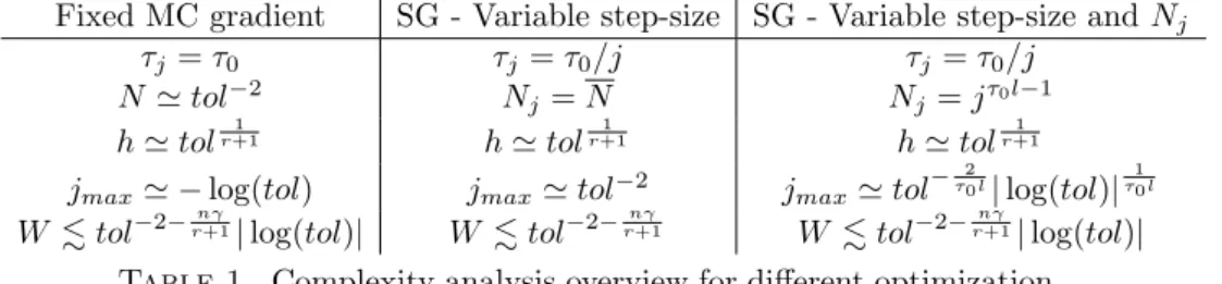
Fixed MC gradient SG - Variable step-size SG - Variable step-size andNj τj =τ0 τj =τ0/j τj =τ0/j N 'tol−2 Nj=N Nj=jτ0l−1 h'tolr+11 h'tol 1 r+1 h'tol 1 r+1

jmax' −log(tol) jmax'tol−2 jmax'tol−

2

τ0l_|log(tol)|τ10l

W _.tol−2−rnγ+1|_log(tol)| _{W .tol}−2−

nγ

r+1 _{W .tol}−2−

nγ

r+1|_log(tol)|

Table 1. Complexity analysis overview for different optimization

methods

Remark 6. Since the constant l may be challenging to estimate in practice, it is often difficult to fulfill the condition τ0 > 1/l. To bypass this difficulty, one could consider the Averaged Stochastic Gradient method[38] instead, in which the step size τj = τ0/jη, η ∈ (0,1) is chosen, with Nj =N and the averaged control

1 j

Pj

i=1ui is considered. The analysis of this alternative method is postponed to a future work.

Table 1 summarizes the results obtained in both the fixed sample size and in-creasing sample size regimes. There, the total work (W) to achieve a given tolerance (tol) is presented. We see from the table that the two considered SG versions im-prove the complexity only by a logarithmic factor compared to the fixed gradient algorithm. The advantage we see in the SG version w.r.t. the fixed gradient, is that we do not have to fix in advance the sample size N and we can just monitor the convergence of the SG iteration until a prescribed tolerance is reached. However, in Algorithm 2, we do have to choose in advance the FE mesh size. It is therefore natural to look at a further variation of the SG algorithm in which the FE mesh is refined during the iterations until a prescribed tolerance is reached. This is detailed in the next Section.

7. Stochastic Gradient with variable mesh size

In this section, we refine the mesh used for our FE approximation, while running the optimization routine. The new mesh size hj is now depending on the iteration

j. Here we study only sequences of nested meshes of sizehj = 2−`(j)with`:N→N

being an increasing function. The optimization procedure then reads:

(40) uhj+1 j+1 =u hj j −τjE −→ ωj M C[∇f hj_(uhj j , ω)], with −→ωj := (ω (1) j ,· · ·, ω (Nj)

j ). Notice that if non-nested meshes are used, a

projec-tion operator should be added in (40) to transfer informaprojec-tion from one mesh to another. We first derive an error recurrence formula in the spirit of (33) for the particular recurrence (40) with a decreasing mesh-size hj.

Theorem 8. Denoting byuhj+1

j+1 the approximated control obtained using the recur-sive definition (40), and u∗ _{the exact control for the continuous optimal problem} (10), we have: (41) E[kuhj+1j+1−u ∗_k2_] ≤cjE[kuhjj −u ∗_k2_{] +} 4τ 2 j NjE [k∇f(u∗, ω)k2_{] + 4τ} j τj(1 + 2 Nj ) +1 l Ch2_jr+2, with cj = 1− τjl 2 +τ 2 jL 2 _{2 +} 2 Nj . 21

Proof. Subtracting the optimal continuous controlu∗ from both sides of the recur-rence formula (40), we get

uhj+1 j+1 −u ∗_=uhj j −u ∗_−τ jE −→ ωj M C[∇f hj_(uhj j , ω)]±τjE[∇f hj_(u∗_)]±τ jG[∇fhj(u hj j )] +τjE[∇f(u ∗_)] =uhj j −u ∗_+τ j E[∇fhj_(u∗_)]−G[∇fhj_(uhj j )] +τj G[∇fhj_(uhj j )]−E −→ ωj M C[∇f hj_(uhj j , ω)] +τj E[∇f(u∗)− ∇fhj(u∗)].

Then setting as in proof of Theorem 6: T1:=G[∇fhj(u hj j )]−E[∇f hj_(u∗_)], T2:=G[∇fhj(u hj j )]−E −→ ωj M C[∇f hj_(uhj j , ω)], T3:=E[∇f(u∗)− ∇fhj(u∗)],

we can rewrite the last equality as: uhj+1 j+1 −u ∗_=uhj j −u ∗_−τ jT1+τjT2+τjT3. We compute the mean of the squared norm of uhj+1

j+1 −u∗ as (42) E[kuhj+1j+1−u ∗_k2_{] =} E[kuhjj −u ∗_k2_{] +τ}2 jE[kT1k 2_{] +τ}2 jE[kT2k 2_{] +τ}2 jE[kT3k 2_] −2τjE[huhjj −u ∗_{, T1i] + 2τ} jE[huhjj −u ∗_{, T2i] + 2τ} jE[huhjj−u ∗_{, T3i]} −2τj2E[hT1, T2i] + 2τj2E[hT2, T3i]−2τj2E[hT1, T3i]. Next, we will bound each of these ten terms to find a recursive formula on_E[kuhj

j −

u∗k2_{]. First, the term τ}2

jE[kT1k2] can be bounded as in the proof of Theorem 6 leading to: τ_j2_E[kT1k2]≤τj2L 2 hjE[ku hj j −u ∗_k2_],

withLhj being the Lipschitz constant for the functionf

hj_{, which is bounded byL} (see Lemma 4). For the termτ_j2E[kT3k2], we find,

τ_j2_E[kT3k2_{] =τ}2 jkE[∇f(u ∗_{)− ∇f}hj_(u∗_)]k2 =τj2kE[p(u∗)−phj(u∗)]k2 ≤τ_j2_E[kp(u∗)−phj_(u∗_)k2_] ≤2τ_j2E[kp(u∗)−pe hj_(u∗_)k2_{] + 2τ}2 jE[kpe hj_(u∗_)−phj_(u∗_)k2_]

≤2Cτ_j2E[|p(u∗)|2Hr+1]h2r+2+ 2Cτ_j2E[|y(u∗)|2_Hr+1]h2r+2 [using C´ea’s Lemma]

≤2τ_j2C(y(u∗), p(u∗))h2r+2. Next, forτ2

jE[kT2k2] we use the same steps as in Theorem 6 to find

τj2E[kT2k2]≤ 2τ_j2L2_hj Nj E h kuhj j −u ∗_k2i₊2τ 2 j NjE h k∇fhj_(u∗_{, ω)k}2i_. Then we bound the second term of the right hand side uniformly w.r.t. hj by

k∇fhj_(u∗_{, ω)k}2_≤2k∇fhj_(u∗_{, ω)− ∇f(u}∗_{, ω)k}2_{+ 2k∇f(u}∗_{, ω)k}2 ≤4C(y(u∗), p(u∗))h2r+2+ 2k∇f(u∗, ω)k2_,

where we have used the same steps as forT3 to boundk∇fhj(u

∗_{, ω)− ∇f(u}∗_{, ω)k.}

Finally, for the cross terms we have 2τjE[huhjj −u ∗_{, T1i] = 2τ} jE[huhjj −u ∗_{, G[∇f}hj_(uhj j )− ∇f hj_(u∗_)]i] = 2τjE[G[huhjj −u ∗_,∇fhj_(uhj j )− ∇f

hj_(u∗_{)i]] [using Strong convexity]} ≥τjlE[kuhjj −u ∗_k2 ], and as in Theorem 9, 2τjE[huhjj−u ∗_{, T2i] = 2τ}2 jE[hT1, T2i] = 2τj2E[hT2, T3i] = 0. Moreover 2τjE[huhjj −u ∗_{, T3i]≤2τ} j l 4E[ku hj j −u ∗_k2 ] +2τj l E[kT3k 2 ] ≤2τj l 4E[ku hj j −u ∗_k2_{] +}4τj l C(y(u ∗_{), p(u}∗_))h2r+2_, and finally 2τ_j2_E[hT1, T3i]≤τj2E[kT1k 2_{] +τ}2 jE[kT3k 2_] ≤τ_j2L2_hjE[kuhjj−u ∗_k2_{] + 2τ}2 jC(y(u ∗_{), p(u}∗_))h2r+2_.

Putting everything together, we finally obtain (41), as claimed. A natural choice to tune the parameters τj,Nj andhj would be to set, guided

by the usual Robbins-Monro theory,τj=τ0/j,Nj =N and balancing all terms on

right hand side of (41).

Theorem 9. Suppose that the assumptions of Corollary 1 hold and letuhj j denote the j-th iterate of (40). For the particular choice (τj, Nj, hj) = (τ0/j, N , h02−`(j)), with `(j) =dln2(j)−ln2(τ0l)

2r+2 e, and assumingτ0>1/l, we have:

(43) _E[kuhj

j −u

∗_k2_]

≤F1j−1 for a suitable constant F1 independent ofj.

Proof. With the choice ofτj,Nj and`(j) in the statement of the theorem, the two

last terms 4τ 2 j NjE[k∇fhj(u ∗_{, ω)k}2_{] and 4τ} j τj(1 +_N2_j) +1_l Ch2_jr+2 in the inequality (41) have the same orderO(j−2_{). Then, we apply the same reasoning as in Theorem}

7 to conclude the proof.

Now we present the idea of the SG algorithm 3 with variable mesh size. Algorithm 3: Stochastic Gradient with variable mesh size algorithm Data:

Given a desired tolerance tol, choose 1_l < τ0,h0 andjmax'tol−2 initialization:

u= 0

forj= 1, . . . , jmax do

update mesh size toh=h02−d

ln2j−_ln2τ0l

2r+2 e

sample one realization aj=a(·, ωj) or the random field

solve primal problem →y(aj, u) on meshh

solve dual problem→p(aj, u) on meshh d

∇J =αu+p(aj, u)

u=u−τjd∇J

end

Concerning the complexity of Algorithm 3, one can derive the following com-plexity result.

Corollary 4. In order to achieve a given tolerance O(tol), i.e. to guarantee that E[kuhjj−u∗k2].tol2, the total required computational work W is bounded by:

W _.tol−2−rnγ+1

Proof. To achievetol2_.jmax−1 requiresjmax'tol−2. Then the total work required

is bounded by W = jmax X p=1 2N h−_pnγ= 2N jmax X p=1 2nγdln2p2−rln2+2τ0le But asdln2p−ln2τ0l 2r+2 e ≤ ln2p−ln2τ0l

2r+2 + 1, one can bound:

W ≤2N jmax X p=1 2nγ ln2p −_ln2τ0l 2r+2 +1 ≤2nγ+1N{τ0l} −nγ 2r+2 jmax X p=1 p2nγr+2 ≤2nγ+1N{τ0l} −nγ 2r+2 2r+ 2 2r+ 2 +nγ(jmax+ 1) nγ 2r+2+1

But asjmax'tol−2, we finally bound the computational work by

W _.tol−2−rnγ+1_.

We notice that the asymptotic complexity remains the same as in the Stochastic Gradient algorithm with fixed mesh size. However, as we only use computations on coarse meshes for the first iterations, we thus expect an improvement due to re-ducing the constant. We will compute this constant, based on numerical examples, in the Section 8.

8. _{Numerical results}

In this section we verify the assertions of Theorems 5, 8, and 9, as well as the computational complexity derived in the corresponding Corollaries. Specifically, we illustrate the order of convergence for the three versions of the steepest descent al-gorithm presented in Sections 5, 6, and 7 respectively. For this purpose, we consider the optimal control problem (19) with a MC approximation of the expectation. We consider problem (2) in the domainD= (0,1)2withg= 1 and the random diffusion coefficient

(44) a(x1, x2,ξ) = 1 + 0.1

ξ1cos(πx2) +ξ2cos(πx1) +ξ3sin(2πx2) +ξ4sin(2πx1)

, with (x1, x2)∈D andξ= (ξ1, . . . , ξ4) withξi

iid

∼ U([−1,1]). Figure 2 shows three typical realizations of the random field. The target function zd has been chosen

as zd(x, y) = sin(2πx) sin(2πy) (see Fig. 1 b) and we have taken α= 0.1 in the

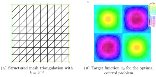
objective function J(u) in (3). For the FE approximation, we have considered a structured triangular grid of size h (see Fig. 1 a) where each side of the domain D is divided into 1/hsub-intervals and used piece-wise linear FE (i.e. r= 1). All calculations have been performed using the FE library Freefem++[20].

(a)Structured mesh triangulation with h= 2−3 IsoValue -1.10526 -0.947368 -0.842105 -0.736842 -0.631579 -0.526316 -0.421053 -0.315789 -0.210526 -0.105263 0 0.105263 0.210526 0.315789 0.421053 0.526316 0.631579 0.736842 0.842105 1.10526 z_d

(b)Target functionzdfor the optimal

control problem

Figure 1. Mesh and target functionzd.

(a)Y1= 0.0327973 Y2= 0.10508 Y3= 0.141335 Y4= 0.905369 (b)Y1= 0.370554 Y2 = 0.0682218 Y3= 0.667794 Y4=−0.421315 (c)Y1=−0.943052 Y2= 0.968895 Y3=−0.656957 Y4=−0.997339

Figure 2. Three realizations of the diffusion random field (44).

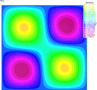
Reference solution. To compute a reference solution of problem (2), we use a full tensorized Gaussian Legendre (GL) quadrature grid with 5 points in each direction and a fine triangulation withh= 2−8(see, e.g., references [8, 37] and Appendix A.2 for a formal error estimate). As this approximated problem is now deterministic with fixed Gaussian nodes, we used a stopping condition on the gradient. In Figure 3 we show the optimal control obtained after j = 6 iterations when the stopping criterionkEGL

(5,5,5,5)[∇J(u h

j)]k ≤10−8 was met, whereuhj is thej-th iterate of (19)

andEbin (19) is a full tensorized Gaussian Legendre (GL) quadrature approximation

of the expectation. The steepest descent step size was chosen asτ0= 10. TheL2 -norm of the final control using this Gaussian quadrature isk_buh=2−8

j=6 k= 0.0663345.

8.1. Steepest descent algorithm with fixed discretization. We investigate here the convergence of the method defined in (24), for which we recall the error bound (30) in the case of piece-wise linear FE (i.e.r= 1):

E[kub h j −uk 2_] ≤C1e−ρj+ C2 N +C3h 4_. 25