ROBUST PRINCIPAL COMPONENT ANALYSIS BASED ON TRIMMING AROUND AFFINE SUBSPACES
C. Croux1, L.A. Garc´ıa-Escudero2, A. Gordaliza2, C. Ruwet3 and R. San Mart´ın2 1KU Leuven,2Universidad de Valladolid and 3HE de la Province de Li`ege
Abstract: Principal Component Analysis (PCA) is a widely used technique for reducing dimensionality of multivariate data. The principal component subspace is defined as the affine subspace of a given dimensiond giving the best fit to the data. PCA suffers from a well-known lack of robustness. As a robust alternative, one can resort to an impartial trimming based approach and search for the best subsample containing a proportion 1−αof the observations, with 0< α <1, and the bestd-dimensional affine subspace fitting this subsample, yielding the trimmed principal component subspace. A population version will be given and existence of solutions to both the sample and population problems will be proven. Moreover, under mild conditions, the solutions of the sample problem are consistent toward the solutions of the population one. The robustness of the method is studied by proving qualitative robustness, computing the breakdown point, and deriving the influence functions. Furthermore, asymptotic efficiencies at the normal model are derived and finite sample efficiencies are studied by means of a simulation study. Key words and phrases: Affine Subspaces, Dimension Reduction, Orthogonal Re-gression, Principal components, Multivariate statistics, Robustness, Trimming.
1. Introduction
When analyzing multivariate data sets, one of the primary goals is to reduce the dimension of the data set at hand with a minimal loss of information. This is often a preliminary step to carry out other statistical analysis such as classifica-tion, regression fits and so on. Principal Component Analysis (PCA) is the most commonly used technique for doing this task and most practitioners of statistics are familiarized with this method due to its intuitive geometrical appealing and its implementation in most of statistical packages. As it happens with many classical statistical methods, one of the main drawbacks of PCA is the lack of ro-bustness against the presence of outlying observations in the data set. There are
a lot of examples in the literature showing that one single outlier, strategically placed, is enough to make classical PCA providing unreliable results.
During the past years, there have been several proposals to robustify classical PCA. Most of them use robust estimates of the covariance matrix and compute eigenvectors and eigenvalues from it. As such, Campbell (1980) and Devlin et al. (1981) use M estimates, Croux and Haesbroeck (2000) take high breakdown point covariance matrix estimators such as the Minimum Covariance Determinant estimator and Croux et al. (2002) use sign and rank covariance matrices. Another approach is based on the “projection pursuit” idea, where one looks for the direction maximizing a robust measure of scale of the data projected on it (Li and Chen, 1985; Croux and Ruiz-Gazen 2005). A hybrid approach combining projection pursuit and robust covariance matrices was followed by Hubert et al. (2005). Robust procedures have also been developed for kernel PCA (see, e.g., Debruyne and Verdonck, 2010 and references therein) or in the learning machine literature (see, e.g., Xu, Caramanis and Sanghavi, 2012 and references therein). In this paper one aims at retrieving directly the lower dimensional affine subspace best fitting the large majority of the data. More precisely, we are looking for the “best” subset of size n− bnαc, with 0≤α <1, hereby trimming a portionα of the data, and the corresponding best fitting affine subspace of a given dimension, where the goodness of fit is measured by the sum of squared Euclidean distances between the subspace and the selected observations. More formally, given a sample X = {x1, ..., xn} of observations in Rp and 0≤α <1,
one looks for the solution of the problem: min
Y⊂X,#Y≥n−bnαch∈Amind(Rp) 1 #Y
X
xi∈Y
kxi−Prh(xi)k2, (1.1)
where Ad(Rp) denotes the set of d-dimensional (1 ≤ d < p) affine subspaces in Rp and Prh(·) denotes the orthogonal projection on h ∈ Ad(Rp). The “best”
subspace according to (1.1) is called the trimmed principal component subspace. The “best” Y with n− bnαc observations is the optimal set which contains the observations surviving the trimming process.
Trimming procedures have revealed as a powerful tool to robustify statistical methods. The idea of discarding a symmetric proportion of extreme observations
in both sides of the sample is a very old and appealing proposal for robustifying the classical univariate sample mean. In order to overcome the implicit hypothesis of symmetry and to extend the idea of trimming to other frameworks such as multivariate estimation and regression, trimming procedures based on the idea of searching for the “best” subsample containing a fixed proportion of the data were introduced by Rousseeuw (1984, 1985). That gave raise to the well known Least Median of Squares (LMS) and Least Trimmed Squares (LTS) procedures in the robust regression context and the Minimum Volume Ellipsoid (MVE) and the Minimum Covariance Determinant (MCD) in the robust multivariate estimation context. Later on, Gordaliza (1991) stated a functional or population version of some related trimming procedures in the multivariate setting and coined the term “impartial trimming” which means that it is the data set itself which tells us the best way of trimming a fixed proportion α of the data.
The problem defined in (1.1) is also considered in Maronna (2005), who pro-posed a fast approximative algorithm to compute its solution. His paper mainly discussed computational aspects, while this paper presents a theoretical study of the trimmed principal component subspace, including existence, consistency, influence function and asymptotic variance of the estimators.
The outline of the paper is as follows. In Section 2, we state the functional version of the problem by using trimming functions and we prove some prelimi-nary results simplifying the problem and throwing light on the way how impartial trimming proceeds in this case. Section 3 is devoted to a general existence result, not requiring any conditions on the distribution. Consistency is proven in Section 4 for absolutely continuous random variables. Special attention is paid to the case of elliptical distributions in Section 5. Robustness aspects are considered in Section 6 including qualitative robustness, influence functions and breakdown point, while asymptotic variances are obtained in Section 7. Section 8 provides finite-sample efficiencies. We also compare the robustness of different robust es-timators for PCA by means of a simulation study. Section 9 contains a data example and we end with a concluding section. All the proofs are deferred to a supplementary file.
2. Notation and preliminary results
space,βpdenotes theσ-algebra of all Borel sets in
Rp,PX the probability measure
induced byX on (Rp, βp) and k · kthe usual norm on Rp. For a set S ⊂Rp, S
denotes its closure, Sc its complementary set and IS(·) its associated indicator function. For 1≤d < p,Ad(Rp) denotes the set ofd-dimensional affine subspaces
inRp and for h∈ Ad(Rp), Prh(·) denotes the orthogonal projection on h.
We recall the notion of “trimming function” introduced in Gordaliza (1991) and used in Cuesta-Albertos et al. (1997). Trimming functions are introduced in order to allow impartial trimming of observations and play an important technical role. For 0≤α <1,Tα =Tα(X) denotes the nonempty set of trimming functions forX at level α, i.e.,
Tα ={τ :Rp→[0,1] measurable,
Z
τ(x)dPX(x) = 1−α},
and Tα−=Tα−(X) denotes the set of trimming functions for level 0≤β ≤α,
Tα−={τ :Rp→[0,1] measurable, Z τ(x)dPX(x)≥1−α}= [ β≤α Tβ.
A more general statement of the Robust Principal Component Analysis problem based on trimming can be given by using trimming functions instead of trimming subsets:
Problem statement: For α∈(0,1) and 1≤d < p, search for a trimming
functionτ0 ∈ Tα− and an affine subspace h0 ∈ Ad(Rp) solution of the problem:
inf τ∈Tα− inf h∈Ad(Rp) 1 R τ(x)dPX(x) Z τ(x)kx−Prh(x)k2dPX(x). (2.1)
The minimum value in (2.1) will be denotedVd,α≡Vd,α(PX)≡Vd,α(X).
We first state some technical results devoted to simplify the problem (2.1) and to make the proofs of the existence and consistency results easier. The next result guarantees the boundedness of the optimal value of the objective function in (2.1). We recall that all proofs can be found in the supplementary file.
Lemma 1 For any1≤d < p and any 0≤α <1, we haveVd,α(X)<∞.
The next lemma shows that the solution in (2.1) is characterized by a strip. Givenh∈ Ad(Rp) and r≥0, we define the strip aroundh and with radiusr as
S(h, r) :={x∈Rp:kx−Pr
Lemma 2 For any h ∈ Ad(Rp) and 0 ≤β < 1, let us denote rβ(h) = inf{r ≥
0 : PX S(h, r) ≤1−β ≤PX S(h, r)} and Th,β ={τ ∈ Tβ :IS(h,rβ(h)) ≤ τ ≤
IS(h,rβ(h)), PX-a.e.}, then, for all τ ∈ Th,β we have:
(a) R
τ(x)kx−Prh(x)k2dPX(x)≤
R
τ0(x)kx−Prh(x)k2dPX(x)for all the
trim-ming functions τ0 ∈ Tβ;
(b) The equality in (a) holds if and only if τ0∈ Th,β.
Takeτh,β any trimming function inTh,β. From Lemma 2 (b) it follows that
Vd,β(h) :=
1 1−β
Z
τh,β(x)kx−Prh(x)k2dPX(x), (2.2)
is the same for every τh,β ∈ Th,β. We call (2.2) the β-trimmed variation of X
aroundh. Unless necessary, no explicit reference to any particular choice inTh,β
will be made and the notationτh,βwill be used for any trimming function inTh,β.
Lemma 2 (a) says that taking another trimming functionτ cannot decrease the value of (2.2). Hence,τh,β, which is essentially an indicator function of the strip S(h, rβ(h)) aroundh, is the optimal trimming function for the problem (2.1).
Lemma 3 With the same notation as in Lemma 2, if β ≤α, we have: (a) Vd,α(h)≤Vd,β(h);
(b) The equality in (a) holds if and only if rα(h) = rβ(h) and PX(S(h, rα(h))) = 0.
It follows from Lemma 3 that, in order to minimize theα-trimmed variation around h, it is strictly better to trim the exact proportionα, except in the case that all the probability mass ofS(h, rα(h)) is supported on its boundary. Lemma
2 and Lemma 3 together result in
Proposition 1 For any h ∈ Ad(Rp) and 0 ≤ α < 1, it holds that Vd,α =
infh∈Ad(Rp)Vd,α(h).
The above proposition allows us to simplify the original double minimization problem (2.1) to the single search of the optimal affine subspace. Once the opti-mal affine subspacehis determined, the optimal trimming function is essentially
the indicator function of the associated stripS(h, rα(h)). Any affine subspaceh0 satisfying Vd,α(h0) = Vd,α, i.e. being a solution of the problem stated in (2.1), will be called a d-dimensional α-trimmed principal component subspace of X. The shorter name trimmed principal component subspace will be also used.
Note that the previous problem statement covers both the population and the sample problem. In the sample casePX is replaced by the empirical measurePnω.
That is, if we have a sample {Xi}ni=1 of size n from the probability distribution
PX, the associated empirical measure is defined as
Pnω(A) = 1 n n X i=1 IA(Xi(ω))
for ω in the sample space Ω. Now, given the outcome of a sample X1(ω) =
x1, ..., Xn(ω) =xn, we can see that the problem stated in (1.1) is equivalent to
the problem (2.1) when takingPω
n instead ofPX.
3. Existence
The main goal of this section is to state the existence of solutions of problem (2.1). The result would guarantee the existence of solutions of both the popu-lation and the sample problem. We do not assume any moment condition on the underlying distribution. This is important in terms of robustness, because outliers are often associated with the presence of heavy tails for the underlying distribution, where moment conditions are not realistic.
From Lemma 1 and Proposition 1, we have that
Vd,α= inf
h∈Ad(Rp)
Vd,α(h)<∞, (3.1)
so we can take a sequence of subspaces {hn}n ⊂ Ad(Rp) such that Vd,α(hn) ↓ Vd,α asn→ ∞. For any affine subspace hn in that sequence, let us denote τn= τhn,α, the radius rn = rα(hn) and Sn = S(hn, rn). Moreover, we parameterize hn through the distance to the origin, denoted by dn = infx∈hnkxk, and the
choice ofdunitary vectors spanning the affine subspace. The boundedness of the sequences{dn}nand {rn}n follows from the following lemma:
Lemma 4 If{hn}nis a sequence of affine subspaces inAd(Rp)satisfyingVd,α(hn)↓ Vd,α as n→ ∞, then {dn}n and {rn}n are bounded sequences.
Furthermore, as all d sequences of unitary vectors are bounded and Rp is
a complete space, {hn}n contains a convergent subsequence in the sense that
the corresponding subsequences of unitary spanning vectors, distances to the origin{dn}n, and the radii{rn}n, are all convergent. We pass to this convergent
subsequence without changing notation. We now state the existence result:
Theorem 1 Let X be a random vector, α ∈ (0,1) and 1 ≤d < p. Then there exists a d-dimensional α-trimmed principal component of X.
Now that existence of the trimmed principal component subspace is estab-lished, we can formulate two important corollaries. The first one says that the optimal trimming function is essentially the indicator function of a strip whose axis is the optimal affine subspace. The second one establishes that the trimmed principal component subspace is spanned by the eigenvectors associated with the largest eigenvalues of the covariance matrix obtained with respect to the probability distributionPX “restricted” through the optimal trimming function.
Corollary 1 Under the hypotheses of Theorem 1, if (τ0, h0) is a solution of (2.1), thenIS(h0,rα(h0))≤τ0≤IS(h0,rα(h0)), PX-a.e. Moreover, ifPX is absolutely continuous w.r.t. the Lebesgue measure on Rp, then IS(h0,rα(h0))=τ0, PX-a.e.
For every τ ∈ Tα, let us denotePXτ the probability distribution induced on Rp by the restriction of X throughτ, i.e. for every Borel set A,
PXτ(A) = 1 1−α
Z
A
τ(x)dPX(x).
Corollary 2 Under the hypotheses of Theorem 1, if τ0 and h0 are a solution of (2.1) and X has finite second order moments, then h0 is the affine subspace spanned by the ordinary principal components of the probability distribution Pτ0
X.
If Corollary 2 would not hold, the α-trimmed variation could be strictly di-minished by replacingh0by the affine subspace spanned by the ordinary principal components of Pτ0
X and thenτ0 and h0 would not be a solution of (2.1). 4. Consistency
While Theorem 1 guarantees the existence of solutions for the population and the sample problems, we now prove the convergence of the sample solutions
to the population ones. The convergence between affine subspaces is stated as the convergence of the distances to the origin and the possible choice of a sequence of converging unitary spanning vectors. Obviously, the sequences of sample optimal radii and sample trimmed variations will then also be consistent.
From now on, {Xn}n is a sequence of Rp-valued r.v. andhn∈ Ad(Rp), n=
1,2, ..., is thed-dimensional trimmed principal component subspace forXn with associated optimal trimming function τn = τhn,α(Xn) and optimal radius rn.
Moreover,Vn:=Vd,α(Xn), n= 0,1,2, ..., denotes the trimmed variation ofXn.
The main result on the consistency of the trimmed principal component subspace is based on a continuity result as well as on the Skorohod representation theorem. This scheme of the proof is similar to that used in Cuesta-Albertos et al. (1997) to establish consistency for trimmedk-means. As in Cuesta-Albertos et al. (1997), difficulties arise since the trimming functions have discontinuities on the boundaries of the corresponding strips. To overcome this, the continuity of the probability distribution of the limit random vector will be imposed.
As in the existence proof, the first step is to show that {hn}n contains a
convergent subsequence by showing that their unitary vectors, the distances to the origin {dn}n and the radii sequences{rn}n are bounded.
Lemma 5 Let{Xn}nbe a sequence ofRp-valued random vectors such thatXn→ X0,P-a.e. Then {dn}n and {rn}n are bounded sequences.
The proof of this lemma is essentially the same as that of Lemma 4. One only needs to take into account that the sequence {Xn}n is tight. Now we are
ready to formulate the “continuity” result:
Theorem 2 Let {Xn}n be a sequence of Rp-valued random vectors, α ∈ (0,1)
and 1 ≤d < p. Let {hn}n ⊂ Ad(Rp) be the sequence of d-dimensional trimmed
principal component of Xn, for n= 1,2, . . . Assume that: (a) Xn→X0, P-a.e.;
(b) PX0 is an absolutely continuous distribution;
(c) h0 is the uniqued-dimensional trimmed principal component ofX0. Then hn→h0 and Vn→V0 as n→ ∞.
We can replace the a.s. convergence condition in Theorem 2 by a convergence in distribution. By applying the a.s. Skorohod representation theorem, there exists a sequence{Yn}n of Rp-valued r.v. such that PX0 ≡PY0, PXn ≡PYn and
Yn→Y0 P−a.s. Hence, by applying Theorem 2 to{Yn}n, it follows that
Corollary 3 Theorem 2 holds if we replace condition (a) by (a0) Xn→X0 in distribution.
Finally, to obtain the desired consistency result, consider a sequence of in-dependent, identically distributed r.v. {Xn}n, with probability distribution PX
and recall that problem stated in (1.1) is equivalent to the problem (2.1) tak-ing Pnω instead of PX. Furthermore, it is well-known that the set Ω0 := {ω ∈ Ω such that Pnω converges in distribution to PX} satisfiesP(Ω0) = 1. Thus, the desired consistency result follows as a simple consequence of Corollary 3:
Theorem 3 Let{Xn}n be a sequence of independent, identically distributedRp
-valued random vectors with distributionPX and let{Pnω} be the sequence of em-pirical probability measures, for any ω∈Ω. Let us assume that PX is absolutely continuous having a uniqued-dimensional trimmed principal component subspace
h0 ∈ Ad. If {hωn}n is a sequence of empirical d-dimensional trimmed principal
components of{Pnω}n, then
hωn →h0,P-a.s. and Vd,α(Pnω)→Vd,α(X),P-a.s.
The consistency result requires the uniqueness of thed-dimensional trimmed principal component subspace, which does not hold in general. The uniqueness property may be guaranteed resorting to certain “geometrical” conditions on the probability distribution PX. In the next section, a uniqueness result is obtained
for elliptically contoured distributions.
5. Uniqueness and Fisher consistency for elliptical distributions
In this section, we focus on the interesting case of the elliptically contoured distributions. We say that a Rp-valued r.v. X follows an elliptical symmetric
distributionX∼Ep(µ,Σ) if it admits a probability density function of the form fX(x) =|Σ|−
1
where h is a positive and non-increasing square integrable function called the radial function. The density f is called unimodal if the radial function h has a strictly positive derivative ˙h. The location parameter of the distribution is µ
and the symmetric positive definite matrix Σ is called the scatter matrix, and is proportional to the covariance matrix if the distribution has a second moment. The ordered eigenvalues of Σ will be denoted by λ1 ≥ ... ≥ λp > 0 and the associated eigenvectors will be v1, ..., vp, respectively. To have uniqueness we
need an additional restriction on the eigenvalues. There needs to be a difference between λd and λd+1, where d is the dimension of the affine subspace we are looking for. The other eigenvalues may coincide. This condition guarantees that the space spanned by the firstdeigenvectors of Σ is uniquely determined:
Theorem 4 LetX be a random vector having an elliptically symmetric distribu-tion as in (5.1), with unimodal density. Let λ1≥...≥λp>0 be the eigenvalues of Σ satisfying λd> λd+1. Then,
(a) For every α > 0 and every d < p, the d-dimensional trimmed principal component subspace of X is unique. That subspace passes throughµ and is spanned by the dlargest eigenvectors of the matrixΣ.
(b) IfX has finite second order moments, then the trimmedd-dimensional prin-cipal component subspace coincides with the ordinary prinprin-cipal component subspace of dimension d.
The proof of the uniqueness result needs the application of a multivariate probability inequality in Davies (1987), which is given in the supplementary file. The theorem above tells us that, at any elliptically symmetric distribution, the trimmed principal component subspace passes through the location parameter
µ and it is spanned by the largest d eigenvectors of the scatter matrix Σ. If the second moment exist, then Σ is proportional to the covariance matrix and, therefore, the principal axis corresponding to the trimmed principal components are the same as those obtained by using the standard PCA.
We also give a Fisher consistency result for elliptical contoured distribu-tions. At this point, some functional notations are needed. To avoid notational complexity, from now on, we omit the reference to the random vector X in the notation PX by just writing P. For a given distribution P with density as in
(5.1), let us denote byS(P) the optimal strip associated with the trimmed prin-cipal component subspace. By Theorem 4 and the hypothesis on the eigenvalues of Σ, this strip is centered at µand has the firstdeigenvectors of Σ as spanning vectors. We define the functional giving us the average over this space
m(P) = 1
1−α
Z
S(P)
xdP(x).
Analogously, we introduce the (restricted) covariance matrix
C(P) = 1
1−α
Z
S(P)
(x−m(P))(x−m(P))0dP(x). (5.2)
Due to orthogonal and translation equivariance of the loss function defining the optimal strip, these functionals are orthogonal and translation equivariant. Based on this property, we restrict our attention to elliptical distributions cen-tered at the origin and with diagonal scatter matrix, i.e. µ= 0 and Σ is a diagonal matrix. In this case, it is easy to see that m(P) = 0 and C(P) is diagonal.
Theorem 5 Let P be with density as in (5.1). If we assume finite second order moments, then there exists a real constant c depending only on the distribution
P via the radial function h and the trimming constant α, such that the first d
eigenvalues and eigenvectors of c C(P) are equal to the first d eigenvalues and eigenvectors of the covariance matrix ofP. At the multivariate normal distribu-tion, one has c= 1.
To get Fisher consistency, the matrix C(P) needs to be multiplied by a constant c. In the sequel, the functional C will always be multiplied by this consistency factorc. At the multivariate normal distribution, no such correction is needed, but at other types of elliptical distributions, c may be different from one.
6. Robustness
6.1. Qualitative Robustness
Hampel (1971) introduces the qualitative robustness of a sequence of esti-mators{Tn}∞n=1 as the equicontinuity of the mappings{P → LP(Tn)}∞n=1, where
He also defines a “continuity” condition for a sequence of estimators at a distri-butionF. IfTn is such thatTn=T(Pnω) with Pnω the empirical distribution, the continuity condition is analogous to that ofT being a weak continuous functional.
Theorem 6 Thed-dimensional trimmed principal component subspace functional is weakly continuous and qualitatively robust at any absolutely continuous distri-bution P having a uniqued-dimensional trimmed principal component subspace. Notice that we need again a uniqueness condition. This condition is similar to that needed for the population median in stating the qualitative robustness of the median estimator or the one needed to state the qualitative robustness of the trimmed k-means estimator in Garc´ıa-Escudero and Gordaliza (1999).
6.2. Influence function
The influence function (IF) is the keystone of Hampel’s infinitesimal ap-proach to Robust Statistics (Hampel 1974 and Hampel et al. 1986). It quantifies the impact than an observation has on an estimator. The IF is a common measure of robustness, also in the context of principal components analysis. Furthermore, it a useful tool for computing asymptotic variances.
Thus, to further investigate the robustness and asymptotic properties of the trimmed principal component subspace estimator, we compute its influence func-tion, for the eigenvalues and eigenvectors, at elliptical contoured distributions. The main ideas will follow Croux and Haesbroeck (1999). The IF of a functional
T at a distribution P is given by IF(x0;T, P) = limε↓0(T((1−ε)P +εδ{x0})−
T(P))/ε, for thosex0 where this limit exists. Here δ{x0} denotes a Dirac distri-bution putting all its mass at x0.
For deriving the influence function of the eigenvectors and eigenvalues at elliptical distributions, we first need the influence function for the functional
C, defined in (5.2). For j = 1, . . . , p, we denote by Λj(P) and Vj(P) the jth
eigenvalue and eigenvector of C(P). Thanks to the orthogonal and translation equivariance of the functional, we may assume thatµ= 0 and take Σ diagonal.
Theorem 7 At an elliptical distribution functionP with probability density func-tion given by (5.1), with µ= 0, and Σ =diag(λ1, . . . , λp), we have that for any
diagonal term of C: IF(x0;C, P)ii= c 1−αIS(P)(x0) x20i− Aii G −Λi(P) + cAii G (6.1)
and for any off-diagonal term (i6=j)
IF(x0;C, P)ij =−
(Λj(P)−Λi(P))λiλj
2(λj−λi)
IS(P)(x0)x0ix0j
Hij .
The quantitiesG, Aii andHij are given in the supplementary file, section (S10). We note that the influence functions are not bounded. This comes from the unboundedness of the stripS(P) along the firstdeigenvectors ofC(P). However, the influence function reveals that only good leverage points, i.e. outliers in the direction of the first deigenvectors and still belonging to S(P), may have huge influence. On the other hand, bad outliers have bounded influence, and their influence is redescending to zero for the non diagonal elements. The influence function is alike the one of the classical estimator for contaminations close to the subspace spanned by the first deigenvectors.
Using the above theorem, one readily obtains the influence functions for eigenvectors and eigenvalues of C. Indeed, for Σ diagonal, Lemma 3 of Croux and Haesbroeck (2000) yields
IF(x0, Vji, P) =
IF(x0, C, P)ji
Λi(P)−Λj(P)
(1−δij)
whereδij is a boolean that takes value 1 whenj=i, and the corresponding result
for eigenvalues IF(x0,Λi, P) =IF(x0, C, P)ii is obtained. For an eigenvector Vi,
with 1≤i≤p, we have that the influence function of its ith component is zero, while for componentj 6=i
IF(x0, Vi, P)j = λjλi λj−λi IS(P)(x0)x0ix0j 2Hij . In another form IF(x0, Vi, P) = X j6=i λiλj λj−λi IS(P)(x0)x0ix0j 2Hij vj, (6.2)
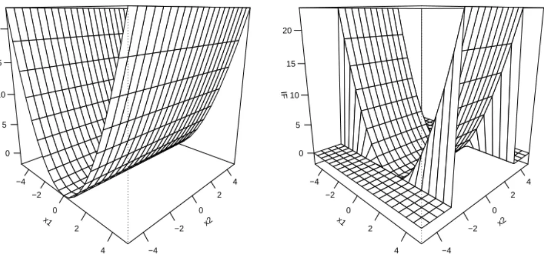
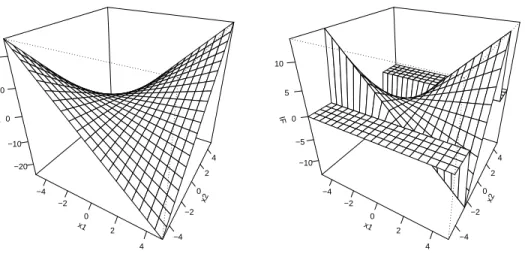
To conclude this section, Figures 6.1 and 6.2 picture the influence functions of the largest eigenvalue and its associated eigenvector for a bivariate normal distribution with zero mean and covariance matrix Σ = diag(2,1). Furthermore, we take d = 1. Only the non-zero component of the influence function of the eigenvector, i.e. only the second component is represented.
x1 −4 −2 0 2 4 x2 −4 −2 0 2 4 IF 0 5 10 15 20 x1 −4 −2 0 2 4 x2 −4 −2 0 2 4 IF 0 5 10 15 20
Figure 6.1: Influence function of the largest eigenvalue at P = N(0,diag(2,1)) when
α= 0 (left panel) andα= 0.01 (right panel).
Inside the strip S(P), which is here given by S(P) ={x2|x22 ≤r2(P)}, the influence function for the untrimmed and the trimmed influence functions have a similar behavior. But outside the optimal strip the influence of the “trimmed” eigenvalue becomes zero, and bounded for the “trimmed” eigenvectors. For the untrimmed or classical eigenvectors and eigenvalues, the influence functions goes beyond all bounds, also outside the optimal strip. The plots illustrate that the trimmed principal components bound the influence of bad leverage points (outside the optimal strip), while they still give unbounded influence to good leverage points. The latter property ensures that the loss in statistical efficiency due to the trimming remains limited, as will be further explored in Section 7.
x1 −4 −2 0 2 4 x2 −4 −2 0 2 4 IF −20 −10 0 10 20 x1 −4 −2 0 2 4 x2 −4 −2 0 2 4 IF −10 −5 0 5 10
Figure 6.2: Influence function of the eigenvector associated to the largest eigenvalue at
P =N(0,diag(2,1)) when α= 0 (left panel) andα= 0.01 (right panel).
The influence function provides just a local description of the behavior of a functional at a probability model and we always need to complement this description with a measure of global reliability. This complementary measure is the breakdown point, that provides a measure of how far from the model the good properties derived from the influence function of the estimator can be expected to extend. We consider Donoho and Huber’s (1983) sample version. Given X ={x1, ..., xn} a sample of npoints and T an estimator based on that
sample, let us denote byε∗n(T,X) the smallest fraction of corrupted observations needed to breakdown the estimatorT, i.e. ε∗n(T,X) = mink/n; supX0kT(X)−
T(X0)k = ∞ , with X0 ranging on the set of all possible samples obtained by replacingkoriginal data points in the sample by arbitrary ones.
We consider the “distance to the origin” of the empirical optimal trimmed principal component subspace based on the sample X. If hX denotes the
em-pirical optimal subspace for the sample, the distance to origin is D(X) := infx∈hXkxk, and we would say that the procedure breaks down when D(X
0)
It is not difficult to see that for the “distance to the origin” estimator as-sociated with classical PCA it suffices to replace d+ 1 data points strategically placed in order to obtain an affine subspace whose distance to the origin is ar-bitrarily large. Hence ε∗n(T,X) = (d+ 1)/n, which asymptotically reaches the worst possible value 0, showing the lack of robustness of the classical estimator. For the trimming based method, the next result shows that the breakdown point of the “distance to the origin” estimator is asymptotically equal toα.
Theorem 8 Let α ∈(0,1/2] and 1 ≤d < p. The breakdown point of the “dis-tance to the origin” estimator D, at any p-dimensional sample X, satisfies
ε∗n(D,X) = min
(bnαc+d+ 1)/n,(n− bnαc)/n →α,as n→ ∞.
Maronna (2005) also analyzed the breakdown point of this procedure. His result coincides with that in Theorem 8 but he focused on the breakdown of the “trimmed scale” target function (i.e., (1.1)) in terms of preventing it to become 0 or ∞ (“implosion” and “explosion”). In our result, we consider a different situation where the whole PCA subspace may be unbounded by taking an arbitrarily large “distance to the origin”. He also introduced an alternative breakdown point concept based on “prediction bias” but he considered that the needed calculations seemed intractable even in the most simple case.
The breakdown point of the “distance to the origin” has its limitation. It considers breakdown due to shifts, but tells nothing about the orientation of the eigenvectors. It might be that the estimated eigenvectors go totally wrong, while the distance to the origin remains bounded. However, the latter type of breakdown is more difficult to formalize and to compute, and we refer to Tyler (2005) for further discussion of the definition of breakdown point for eigenvectors.
7. Asymptotic variances
Under the hypothesis that a functionalT is Frechet differentiable, its asymp-totic distribution is gaussian, and its asympasymp-totic variance is given by
ASV(T, P) = Z
Rd
IF(x, T, P)IF(x, T, P)0dP(x).
expressions of the influence function in section 6.2 allow us to compute the asymp-totic variance in a rather easy way.
7.1. Asymptotic variances in the elliptical case
For an elliptical contoured distribution withµ= 0 and Σ =diag(λ1, . . . , λp), from (6.1) and (6.2), we can obtain the following expressions for the asymptotic variances for the associated eigenvalues and eigenvectors estimators:
ASV(Λi, P) = c2 (1−α)2 Z S(P) x4i|Σ|−12h(x0Σ−1x)dx−Λi(P)2 + α 1−α cAii G 2 + 2Λi(P) cAii G ( −α 1−α) and ASV(Vi, P) =X j6=i λ2iλ2j (λi−λj)2 R S(P)x2ix2jdP(x) 4H2 ij vjvj0, (7.1)
where the quantitiesG, Aii and Hij are again those given in the supplementary
file.
7.2. Asymptotic relative efficiencies in the gaussian case
Using the preceding results, one may obtain information on the efficiency of the estimators of the eigenvectors and eigenvalues ofCcomputed after trimming. We restrict our attention here to gaussian distributions, where further simplifi-cations in the expressions derived for the asymptotic variances can be made. Furthermore, we only consider the first d eigenvalues and eigenvectors (which are also the only once retained in practical data analysis).
In Section 5, we showed that the consistency factor c is equal to 1 for thed
first eigenvalues, and that Λi(P) =λi.These results allow for simpler expressions
of the asymptotic variances of the eigenvalues with 1≤i≤das:
ASV(Λi, P) =
2 1−αλ
2
i. (7.2)
For the eigenvectors with 1≤i≤d, we obtain:
ASV(Vi, P) = 1 1−α X j6=i λiλjcj (λi−λj)2 vjvj0 (7.3)
withcj defined as c−j1 = R S(P)x 2 jdP(x) (1−α)λj . (7.4)
The availability of asymptotic variances under closed form expressions allows us to compute asymptotic relative efficiencies (ARE) with respect to maximum likelihood (ML) estimators at the gaussian model. Note that the ML estimator is the untrimmed PCA and its asymptotic variances are given by the above expressions forα= 0. So it follows from (7.2) that, for 1≤i≤d
ARE(Λi, P) = ASV(ΛM L;i, P) ASV(Λi, P) =
2
2/(1−α) = 1−α,
meaning that, for the firstdeigenvalues, the efficiency is just the complementary of the trimming proportion. For instance, a trimming level of 10% yields a 90% efficiency for the eigenvalue estimators.
Regarding eigenvectors, we have from (7.3) that
ARE(Vi, P) = trace(ASV(VM L;i, P)) trace(ASV(Vi, P)) = P j6=i λj (λi−λj)2 1 1−α P j6=i λjcj (λi−λj)2 .
We evaluate the above expression for the spherical noise situation, where the
p−dlast eigenvalues are assumed to be equal, say, toλ. Observations generated by a spherical noise model are lying in the same subspace, with some spherical noise added. Using (7.4), one can readily see that cj = 1 for j ≤d, and cj = ˜c
forj > d, with ˜c−1=E[Z12I(kZk ≤r˜)] and ˜r2 the 1−αquantile of a chi-square distribution with p−d degrees of freedom. The constant ˜c is the same as the consistency factor needed for the Minimum Covariance determinant estimator computed in Croux and Haesbroeck (1999, p.165). We get
ARE(Vi, P) = (1−α) P j6=i,j≤d λj (λi−λj)2 + (p−d)(λi−λλ)2 P j6=i,j≤d λj (λi−λj)2 + (p−d)˜c(λi−λλ)2 .
This result calls for a few remarks. Globally, the efficiency is again determined by the trimming proportion. But here, other effects appear. For instance (i) If the noise level tends to zero, or λ ↓ 0, the efficiency tends to 1−α; (ii) If the eigenvalue λi gets closer to the noise level λ, the efficiency decreases to
components; (iii) If the space dimensionp rises for fixed model dimensiond, the efficiency reaches 1−α for very high space dimensions, since ˜ctends to 1 with p
going to infinity; (iv) If, everything else being fixed, the model dimensiondrises, numerical computations show that the efficiency increases in almost all scenarios (except for high trimming levels and low initial noise dimension).
8. Simulations
This section studies the finite sample performance of the trimmed PCA. The simulation experiment consists ofm= 1000 replications ofp-dimensional samples of size n with p = 5 or p = 8 and n = 50,100,500 or 1000. The samples were generated according to a normal distribution with a zero mean and a diagonal covariance matrix Σ = diag(λ1, . . . , λp). Two sets of diagonal elements were
considered, similar as in Maronna (2005), representing:
(a) a smooth decrease of the eigenvalues, i.e. λj = 2p−j for 1≤j≤p;
(b) an abrupt decrease of the eigenvalues afterλd, i.e. λj = 20(1+0.5(d−j+1)) for 1≤j ≤dand λj = 1 + 0.1(p−j+ 1) ford+ 1≤j ≤p.
For each dataset, the d-dimensional α-trimmed PCA method was applied with
d= 3, or 7 and α= 0.05,0.1 or 0.25.
The computation of the empirical d-dimensional α-trimmed PC has a high computational complexity, since one needs to optimize over the space of all sub-sets of a given size. Exact algorithms are, in general, no longer possible. In the simulation study that follows, the approximative algorithm of Maronna (2005) is used. This algorithm follows the rationale behind the fast-MCD algorithm in Rousseeuw and van Driessen (1999) for computing the Minimum Covariance Determinant (MCD) estimator, combining random starts and so-called “concen-tration” steps. We recommend to take the number of initial random starts equal to 500, and the number of concentration steps equal to 10.
8.1 Finite-sample efficiencies
In this subsection we verify whether the asymptotic variances of the estima-tors, computed in Section 7, are confirmed by their finite sample counterparts.
To assess the performance of the estimators of the eigenvalues and eigenvec-tors, mean squared error (MSE) were computed. For the eigenvalues, a correction
for bias is first applied and then the classical definition of MSE is used: MSE(Λj) = 1 m m X i=1 (λˆˆ(ji)−λj)2 whereλˆˆ(ji)= ˆλ(ji)×1 m Pm k=1λˆ (k) j /λj −1
and ˆλ(ji) is the estimate ofλj computed
from the ith generated sample. For the eigenvectors, following Croux et al. (2002), the MSE is defined as
MSE(Vj) = 1 m m X i=1 cos−1|vtjvˆj(i)|2
where ˆvj(i) is the estimate of vj computed from theith generated sample. From the MSE values, relative finite sample efficiencies are computed as
Effn(Λj) = ASV(ΛM L;j, P) nMSE(Λj) and Effn(Vj) = trace(ASV(VM L;j, P)) nMSE(Vj) .
These finite sample efficiencies are reported in Table 8.1. Since the efficiencies for the different eigenvalues of a particular setting are quite similar, their average value is reported. In this table, the asymptotic relative efficiencies derived in the previous section appear in the rows referred as “n=∞”.
We first discuss the results for the model with smoothly decreasing eigenval-ues. As we can see from Table 8.1, p = 5, d = 3, the efficiency decreases with an increasing trimming size. The finite sample efficiency of the eigenvalues tends to decrease towards the asymptotic value, while they increase for the eigenvec-tors towards the limit value with increasing sample size. The results for p = 8, where the trimming size is 0.25, show that if the model dimension dincreases, everything else being fixed, a small increase in the efficiency of the eigenvec-tors is observed. This behavior has already been pointed out when studying the asymptotic efficiencies.
Under design (b), there is a large difference between the noise and non-noise levels. The convergence towards the asymptotic efficiencies is here slower than for simulation design (a). Note that some finite sample efficiencies are larger than one, which is possible since they are computed relative to the asymptotic variance of the ML estimator. The ML estimator itself also has finite sample efficiencies larger than one in these cases (see supplementary file). Forp= 8, d= 7 the finite
Table 8.1: Finite sample efficiencies for the trimmed PCA w.r.t. the ML. Design (a) p d α n Eigenvalues Eigenvectors 5 3 .05 50 .992 .754 .677 .590 100 .979 .918 .845 .710 500 .942 .927 .900 .852 ∞ .950 .932 .922 .846 5 3 .10 50 .985 .652 .608 .502 100 .912 .762 .782 .650 500 .905 .828 .809 .710 ∞ .900 .869 .853 .736 5 3 .25 50 .837 .458 .428 .356 100 .761 .586 .554 .436 500 .762 .662 .630 .476 ∞ .750 .689 .659 .483 8 3 .25 50 .806 .497 .447 .356 100 .762 .565 .513 .429 500 .722 .665 .654 .527 ∞ .750 .692 .665 .502 8 7 .25 50 .816 .532 .476 .444 .457 .427 .393 .353 100 .791 .628 .629 .605 .593 .603 .554 .446 500 .770 .755 .732 .714 .698 .689 .643 .517 ∞ .750 .746 .746 .742 .733 .712 .654 .435 Design (b) p d α n Eigenvalues Eigenvectors 5 3 .05 100 1.275 .697 .642 .642 500 1.040 .688 .702 .851 1000 .951 .899 .927 .967 ∞ .950 .950 .950 .949 5 3 .10 100 1.196 .686 .593 .546 500 .919 .689 .665 .713 1000 .923 .831 .829 .882 ∞ .900 .899 .899 .898 5 3 .25 100 1.026 .623 .564 .511 500 .813 .495 .485 .561 1000 .778 .651 .651 .678 ∞ .750 .749 .749 .747 8 3 .25 100 1.009 .614 .541 .485 500 .808 .541 .542 .618 1000 .752 .685 .669 .709 ∞ .750 .748 .748 .745 8 7 .25 100 1.523 1.253 1.306 1.094 .858 .669 .536 .479 500 .969 .598 .521 .473 .485 .532 .572 .590 1000 .866 .547 .505 .516 .552 .601 .641 .691 ∞ .750 .750 .750 .750 .750 .750 .749 .747
sample efficiencies first decrease, and then increase again withn. We do not have an explanation for this, but the same behavior is found for the untrimmed PCA.
8.2 Robustness at finite samples
In this subsection we generate samples containing outliers in order to study the robustness of the estimators at finite samples. Trimmed PCA is compared with 5 other approaches: (i) the ROPCA method of Hubert et al. (2005) (ii) the eigenvectors of the Minimum Covariance Determinant estimator (iii) the Projection Pursuit (PP) approach of Li and Chen (1985) (iv) the eigenvectors of the Sign Covariance Matrix (v) the eigenvectors of the sample covariance matrix. We use the implemented of the rrcov R-package, see Todorov and Filzmoser (2009). Similar simulation studies were carried out in Maronna (2005) and Engelen et al. (2005), among others.
We generate M = 1000 samples of size n, where n− bnc of the data are generated by the model distribution N(0,Σ), with Σ as in the previous subsec-tion. The bncoutliers follow a N(101p,10Σ0), where Σ0 equals Σ with reversed diagonal elements, and 1p a vector of length p only ones. The outliers are at a
large distance from the true principal component space, and also far away from the main data cloud. Hence they are bad leverage points. We performed similar experiments for good leverage points and vertical outliers, yielding comparable relative performance of the different methods. The percentage of outliers varies from 5% to 20%. For the trimmed PCA, we selected α = 0.25 yielding a good compromise between robustness and efficiency. As performance criterion we take the expected squared distance between an observation from the model and the estimated subspace. We compute it as
D2= Trace Σ p X j=d+1 ˆ vjvˆjt
The lowed D2, the better. Figure 8.3 presents the D2, averaged over the M
simulation runs, for the representative case n= 50,p= 5,d= 3, and design (a). If no outliers are present, so = 0, then the sample covariance matrix gives For reasons of comparability between methods, we let the estimated subspace pass the true center of the distribution.
0.00 0.05 0.10 0.15 0.20 3 4 5 6 7 8 % of outliers Exp e ct e d Sq u a re d D ist a n ce Trimmed ROBPCA MCD PP Sign Classic
Figure 8.3: Simulated value ofD2as a function of the percentage of outliers for 6 different
estimators, for design (a) withn= 50,p= 5, andd= 3.
the best results, but its performance deteriorates quickly. The robust estimators are much more stable under contamination; the PP and the Sign covariance matrix start to perform worse in presence of outliers, but they do not explode. The Trimmed PCA, the MCD and ROBPCA yield the best results, where the
D2 does not increases further when outliers are added (the reason for this is that the more outliers there are, the less good observations are trimmed away). The ROBPCA method gives very good results, in line with previous simulation studies. ROBPCA is documented to work very well in practice, but no theoretical results are available for this approach. The MCD and the trimmed PCA method perform similar in this experiment, and are not too far from the ROBPCA. It is not surprising that MCD and trimmed PCA give similar results, since both yield eigenvectors from sample covariances matrices computed from trimmed samples. But trimmed PCA is the more natural approach in this setting, and it can also be computed for n < p or when a majority of the data is lying exactly on a subspace.
esti-mator over a larger range of outlier positions. We find that (i) the performance of the robust estimators is deteriorating if is getting larger (ii) intermediate outliers may be more dangerous than extreme outliers.
9. Data Example
In this section we illustrate the method using the Breast cancer data set, described in Chin et al. (2006) and available in the R-package PMA. We take the p = 20 comparative genomic hybridization (CGH) variables with largest standard deviation, measured forn= 89 patients for the first chromosome. Aim is to visualize the patients in a plane, and therefore we look for the optimal subspace of dimensiond= 2. Outliers are to be expected in such datasets, and we takeα= 0.25 trimming level. In Figure 9.4 we plot the data projected on the trimmed principal subspace, together with a 95% tolerance ellipse. The tolerance ellipse uses the firstd= 2 estimated eigenvalues. We add a plot of the squared distances of each observation to the α trimmed principal component subspace. We compare the outcomes of the trimmed case (α = 0.25, top figure) and the non trimmed case (α = 0, bottom figure). The different robust PCA methods give comparable results on this example.
We see from Figure 9.4 that the non trimmed approach gives a more spher-ical tolerance ellipsoid, and only one observation is detected as outlying in the subspace. The trimmed approach finds a subspace fitting well the large major-ity of the data; some observations have an unusual large distance (see top right panel) and may be atypical. The horizontal dashed line, that can be used as an heuristic device to diagnose observations with an unusual high distance, corre-sponds to the 95% critical value of a chi-squared distribution with the degrees of freedom estimated by the trimmed variation around the optimal subspace.
10. Conclusions
Principal Component Analysis (PCA) is a technique for reducing dimen-sionality in multivariate data analysis. For p-dimensional observations, and a given dimensiond, withdtypically much lower thanp, classical PCA yields the best fitting affine subspace of dimension d, in the sense of minimizing the sum of squared Euclidean distances between the subspace and the observations. The robust alternative studied in this paper relies on an impartial trimming based ap-proach, where a proportionαof the observations is discarded, and the best fitting
Trimmed −2 −1 0 1 2 −2 −1 0 1 2 v1 v2 0 20 40 60 80 0 .0 0 .5 1 .0 1 .5 2 .0 2 .5 Index d ist a n ce ^2 Not trimmed −2 −1 0 1 2 −2 −1 0 1 2 v1 v2 0 20 40 60 80 0 .0 0 .5 1 .0 1 .5 2 .0 2 .5 Index d ist a n ce ^2
Figure 9.4: Projection on theα-trimmed optimal subspace (left) and squared distances (right) for 89 patients and p= 20. The top plot is for α= 0.25, the bottom plot for
α= 0.
d-dimensional affine subspace is determined from the non-discarded observations. The difficulty is to find this “best” subsample of observations yielding the “best” affine subspace, called the trimmed PC subspace. While an algorithm for com-puting the trimmed PC subspace was already proposed by Maronna (2005), its theoretical properties were not studied yet.
As a first result, we prove existence of the trimmed PC subspace without making any moment restrictions. While standard PCA requires existence of sec-ond moments, this is not required for its trimmed version. Hence, the trimmed PC subspace exists at a multivariate Cauchy distribution, for example, where standard PCA is not feasible. We also prove, under mild conditions, consistency
of the sample trimmed PC space towards the population counterpart. The ro-bustness of the method is studied by showing qualitative roro-bustness, computing the breakdown point, and deriving the influence functions, which turn out to be bounded for bad leverage points. Good leverage points still may have an un-bounded influence. Furthermore, asymptotic efficiencies at the normal model are derived, while finite sample efficiencies of the estimators are obtained by means of a simulation study. It is shown that, by selecting an appropriate trimming proportionα, both a high breakdown point and a high efficiency are attainable. A distinct feature of the proposed method compared to other approaches for robust PCA is that it directly aims at finding the best fitting affine subspace. The population version, which we presented in Section 2 and of which we showed existence in Section 3, has a clear geometric interpretation, also at non-elliptical distributions. If one would use, for example, the space spanned by the first d
eigenvectors of a robust estimate of the covariance matrix as best fitting sub-space, then it is not clear whether the corresponding population quantity has any optimality property, unless at elliptically symmetric distributions. When the aim of the robust principal component analysis is to perform dimension re-duction and to find an optimal subspace of a certain dimension, then trimmed PCA is a natural candidate. A plot of the values of the trimmed variation as a function of dcan be used to select the dimension of the subspace. If such a plot indicates that not much further reduction in trimmed variation can be gained by increasingdtod+ 1, the corresponding dimension can be selected.
Maronna (2005) conducted a simulation study and did found good perfor-mance of the method. He also applied it on several real data sets. An appli-cation in robust multivariate error-in-variables modeling was studied in Croux et al. (2009). Serneels and Verdonck (2009) showed its good performance when applied to principal component regression for data containing outliers.
There are several extensions possible of the trimmed principal components method we studied. One could consider general penalty functions Φ(·) for quan-tifying the discrepancy between the point x and the affine subspace h through Φ(kx−Prh(x)k), instead of merely considering the squared loss. As in
Garc´ıa-Escudero and Gordaliza (1999), we expect that the main robustification arises from the trimming and less by the different choices of the penalty function Φ. We
can also adopt a “min-max” orL∞ approach. In other words, we would search
for the narrowest strip (i.e., having the smallest radius as possible) including a 1−α proportion of the data points. Notice that Rousseeuw’s LMS regression estimator also shares that idea. Applications of the trimming approach in the multiple population case are in robust linear clustering (Garc´ıa-Escudero et al., 2009) and robust cluster analysis (Garc´ıa-Escudero et al., 2008).
Acknowledgment
We would first to thank the Editor, associate Editor, and referees for their comments and suggestions that helped improving the paper. The research of L.A. Garc´ıa-Escudero and A. Gordaliza was partially supported by the Spanish Minis-terio de Ciencia e Innovaci´on, grant MTM2014-56235-C2-1-P, and by Consejer´ıa de Educaci´on y Cultura de la Junta de Castilla y Le´on, grant VA212U13.
References
Billingsley, P. (1986), Probability and Measure (2nd Ed.), New York: Wiley. Campbell, N.A. (1980), “Robust Procedures in Multivariate Analysis I: Robust
Covariance Estimation”, J. R. Stat. Soc. Ser. C. Appl. Stat.,29, 231-237. Chin, K., DeVries, S., Fridlyand, J., Spellman, P., Roydasgupta, R., Kuo, W., Lapuk, A., Neve, R., Qian, Z., Ryder, T., et al. (2006). “Genomic and tran-scriptional aberrations linked to breast cancer pathophysiologies”, Cancer Cell, 10, 529-541.
Croux, C., Filzmoser, P. and Fritz, H. (2013), “Robust Sparse Principal Com-ponent Analysis”, Technometrics, 55, 202-214
Croux, C. and Haesbroeck, G. (1999), “Influence function and efficiency of the minimum covariance determinant scatter matrix estimator”, J. Multivari-ate. Anal., 71, 161-190.
Croux, C. and Haesbroeck, G. (2000). “Principal component analysis based on robust estimators of the covariance or correlation matrix: Influence func-tions and efficiencies”, Biometrika, 87, 603-618.
Croux, C., Ollila, E. and Oja, H. (2002). “Sign and Rank covariance matrices: Statistical properties and applications to principal components analysis”, Statistical data analysis based on the L1-norm and related methods (Neuch-tel, 2002), Statistics for Industry and Technology, 257269.
Croux, C., and Ruiz-Gazen, A. (2005), “High Breakdown Estimators for Prin-cipal Components: the Projection-Pursuit Approach Revisited”, J. Multi-variate. Anal., 95, 206-226
Croux, C., Fekri, M. and Ruiz-Gazen, A. (2009), “Fast and Robust estimation of the Multivariate Errors in Variables Model,” Test, 19, 286-303.
Cuesta-Albertos, J.A. and Matr´an, C. (1988), “The Strong Law of Large Num-bers for k-Means and Best Possible Nets of Banach Valued Random Vari-ables”, Probab. Theory Relat. Fields, 78, 523-534.
Cuesta-Albertos, J.A., Gordaliza, A. and Matr´an, C. (1997), “Trimmed k -means: An attempt to robustify quantizers”, Ann. Statist., 25, 553-576. Cuesta-Albertos, J.A., Gordaliza, A. and Matr´an, C. (1998), “Trimmed best
k-nets: A robustified version of an L∞-based clustering method”, Statist.
Probab. Lett., 36, 401-413.
Cuesta-Albertos, J.A., Garc´ıa-Escudero, L. A. and Gordaliza, A. (2002), “On the Asymptotics of Trimmed Bestk-Nets”,J. Multivariate. Anal.,82, 486-516.
Davies, P.L. (1987). “Asymptotic behaviour of S-estimates of multivariate lo-cation parameters and dispersion matrices”,Ann. Statist., 15, 1269-1292. Debruyne, M. and Verdonck, T. (2010), “Robust kernel principal component
analysis and classification”, Adv. Data Anal. Classif.,4, 151-167.
Devlin, S.J., Gnanadesikan, R. and Kettering, J.R. (1981), “Robust Estima-tion of Dispersion Matrices and Principal Components”, J. Amer. Statist. Assoc.,76, 354-362.
Donoho, D.L. and Huber, P.J. (1983), The notion of breakdown point. In: Bickel, P., Doksum, K. and Hodges Jr. J.L., eds., A Festschrift for Erich L. Lehmann. Wadsworth, Belmont, CA.
Engelen, S., Hubert, M. and Vanden Branden, K. (2005) “A comparison of three procedures for robust PCA in high dimensions”,Austrian Journal of Statistics, 34, 117-126.
Garc´ıa-Escudero, L.A. and Gordaliza, A. (1999), “Robustness Properties of k -Means and Trimmed k-Means’,’ J. Amer. Statist. Assoc., 94, 956-969. Garc´ıa-Escudero, L. A., Gordaliza, A., Matr´an, C. and Mayo-Iscar, A. (2008),
“A general trimming approach to robust cluster analysis”, Ann. Statist., 36, 1324-1345.
Garc´ıa-Escudero, L. A., Gordaliza, A., San Mart´ın, R., Van Aelst, S. and Zamar, R. (2009), “Robust linear clustering”, J. R. Statist. Soc. B,71, 301-318. Gordaliza, A. (1991), “Best approximations to random variables based on
trim-ming procedures”,J. Approx. Theory, 64, 162-180.
Hampel, F.R. (1971), “A General Qualitative Definition of Robustness”, Ann. Math. Statist., 42, 1887-1896.
Hampel, F.R. (1974), “The Influence Function and its Role in Robust Estima-tion”, J. Amer. Statist. Assoc.,69, 383-393.
Hampel, F.R., Rousseeuw, P.J., Ronchetti, E. and Stahel, W.A. (1986), Robust Statistics, The Approach Based on The Influence Function, New York: Wiley.
Hubert, M., Rousseeuw, P.J., and Vanden Branden, K. (2005), “ROBPCA: A new approach to robust principal component analysis”, Technometrics,47, 64-79.
Li, G., and Chen, Z. (1985), “Projection Pursuit Approach to Robust Dispersion Matrices and Principal Components: Primary Thery and Monte Carlo”,J. Amer. Statist. Assoc., 80, 759-766.
Maronna, R. (2005). “Principal Components and Orthogonal Regression Based on Robust Scales”, Technometrics,47, 264-273.
Rousseeuw, P.J. (1984). “Least median of squares regression”, J. Amer. Statist. Assoc.,79, 871-880.
Rousseeuw, P.J. (1985). “Multivariate Estimation with High Breakdown Point”, in Mathematical Statistics and Applications, edited by W. Grossmann, G. Pflug, I. Vincze, and W. Wertz, Reidel Publishing Company, Dordrecht, 283-297.
Rousseeuw, P.J. and Van Driessen, K. (1999), “A Fast Algorithm for the Mini-mum Covariance Determinant Estimator”, Technometrics, 41, 212-223. Serneels, S., and Verdonck, T. (2009) “Principal component regression for data
containing outliers and missing elements”, Comput. Statist. Data Anal., 53, 3855-3863.
Todorov, V., and Filzmoser, P. (2009) “An object-oriented framework for robust multivariate analysis”,Journal of Statistical Software, 32, 1-47..
Tyler, D. (2005) “Breakdown and Groups-Discussion”,Annals of Statistics,33, 1009-1015.
Xu, H., Caramanis, C., and Sanghavi, S. (2012), “Robust PCA via Outlier Pursuit”, IEEE Trans. Inform. Theory, 58, 30473064.
KU Leuven, Naamsestraat 68, B3000 Leuven, Belgium. E-mail: ([email protected])
IMUVA y Departamento de Estad´ıstica e Investigaci´on Operativa, E.I.I., Universidad de Valladolid, Paseo del Cauce, 59, 47011 Valladolid, Spain.
E-mail: ([email protected])
IMUVA y Departamento de Estad´ıstica e Investigaci´on Operativa, E.I.I., Universidad de Valladolid, Paseo del Cauce, 59, 47011 Valladolid, Spain.
E-mail: ([email protected])
Haute ´Ecole de la Province de Li`ege (HEPL), Categorie technique, Quai Gloesener, 6, B4000 Li`ege, Belgium.
E-mail: ([email protected])
Departamento de Estad´ıstica Investigaci´on Operativa, E.T.S.I.A., Universi-dad de Valladolid, Avda. Madrid, 57, 34004 Palencia, Spain.