Robust estimation of (partial) autocorrelation

(1)

SFB

823 Robust estimation of (partial)

autocorrelation

Discussion Paper

_{Alexander Dürre, Roland Fried,}

Tobias Liboschik

(2)

(3)

SFB 823 Discussion Paper 12/14 April 7, 2014

Robust estimation of (partial) autocorrelation

Alexander Dürrea,∗_{, Roland Fried}a_{, Tobias Liboschik}a

a_{TU Dortmund University, Department of Statistics, Germany}

Abstract

The autocorrelation function (acf) and the partial autocorrelation function (pacf) are elementary tools of linear time series analysis. The sensitivity of the conventional sample acf and pacf to outliers is well known. We review robust estimators and evaluate their performances in different data situations considering Gaussian scenarios with and without outliers in a simulation study.

Keywords: Autocovariance, outliers, time series, correlogram

1. Introduction

The autocorrelation function (acf) and the partial autocorrelation function (pacf) are elementary tools of linear time series analysis. The graphical presentation as a correlogram gives an idea of the linear dependencies between pairs of observations in different time lags. A sinusoidal shape indicates a seasonality, whereas a slowly decaying function points at possible long range dependence or non-stationarity. Besides descriptive purposes, the autocorrelation and the autocovariance function (Brockwell, 2009) can be used for model identification (see Box et al., 1994, pp. 184–188), for fitting autoregressive models using the Yule-Walker equations, for determining the periodogram (see, e.g., Brockwell and Davis, 2006, pp. 234–238, and Wei, 1990, pp. 265–267), for detecting periodicities (Vecchia and Ballerini, 1991), for clustering or classifying time series (Caiado et al., 2006), and for predicting future values of the time series (Brockwell, 2009).

The sensitivity of the conventional estimators, the sample acf and pacf, to outliers is well known (see Chan, 1992, Deutsch et al., 1990, or Maronna et al., 2006, pp. 247–257). A single outlier can drive the sample autocorrelation at every time lag h towards zero, whereas h+ 1

or more successive outliers can make it arbitrarily close to one, both making the estimation worthless. Several robust alternatives have been proposed in the literature to overcome this problem. We review such approaches and evaluate their performances in different data situations. We aim at some guidance which estimator to apply in which data situation.

∗_{Corresponding author}

Email addresses: [email protected](Alexander Dürre),

[email protected](Roland Fried),[email protected](Tobias Liboschik)

(4)

Section 2 introduces some notation and background which will be used to describe the robust procedures for estimating the acf and pacf in Section 3. Section 4 presents simulations to asses the accuracy and robustness of these estimators, while Section 5 draws some conclusions.

2. Background and Notation

Let (Xt)t∈Z denote a real-valued time series. We assume (Xt)t∈Z to be second order stationary, meaning that the mean and the variance are constant and do not depend on the observation timet, i.e. E(Xt) =µand Var(Xt) =σ2 <∞ for allt ∈Z, while the

autocovari-ance and hence the autocorrelation depend on the time lag only, i.e. Cov(Xt+h, Xt) =γ(h)

and Cor(Xt+h, Xt) =ρ(h) for all t, h ∈Z. Because of ρ(h) = ρ(−h), only positive time lags

h∈_N0 need to be considered. Both the autocovariance and the autocorrelation function of a

stationary process are always positive-semidefinite, i.e., for every k∈_N the matrix

Γ(k) = (Γ(_i,jk))i,j=1,...,k+1 with Γ

(k)

i,j =γ(i−j) (1)

is positive-semidefinite. For a stationary time series the usual relation Cor(Xt+h, Xh) = Cov(Xt+h, Xt) p Var(Xt+h)·Var(Xt) implies ρ(h) = γ(h) γ(0). (2)

This allows us to translate estimators of the autocovariances into estimators of the autocor-relations and vice versa, if an estimate of the varianceγ(0) is available.

For a vector of observations X = (X1, . . . , Xn), let X be the arithmetic mean, Xe_p the p-quantile, 0 < p < 1, and Xe = Xe₀_.₅ the sample median. Furthermore, let X₍₁₎, . . . , X₍_n₎

denote the ordered sample in ascending order and Rt the rank ofXt, t= 1, . . . , n.

The sample analogues ofγ(h) and ρ(h) are the empirical or sample autocovariances and autocorrelationsγˆ(h) and ρˆ(h) (in the simulation study abbreviated as: emp. acf), which are given by ˆ γ(h) = 1 n n−h X t=1 (Xt−X)(Xt+h−X), (3) ˆ ρ(h) = γˆ(h) ˆ γ(0), h∈N .

The denominator n is used in the formula forγˆ(h) instead of the more intuitive number of cross-productsn−h, since this guarantees positive-semidefiniteness of the resulting functions

ˆ

γ and ρˆfor the price of an increased bias. In Schlittgen and Streitberg (2001, p. 244) an asymptotic formula for the bias of the sample acf of Gaussian processes is derived:

Bias( ˆρ(h)) =−1 n hρ(h) + ∞ X i=−∞ ρ(i) + 2ζ(h) ! (1−ρ(h)) ! +O(n−2), (4)

(5)

where ζ(h) =P∞_i₌_−∞ρ(i)ρ(i+h). Equation (4) indicates that a small n and a large positive, slowly decaying acf cause a large negative bias. The estimator is asymptotically unbiased for fixed h asn goes to infinity. The asymptotic distribution of the sample autocorrelation can be found for example in Brockwell and Davis (2006, Theorems 7.2.1 & 7.2.2). Calculation of the empirical acf is recommended only for n ≥50 and h≤n/4 (Box et al., 1994, p. 32).

The sample acf can also be derived from a multivariate covariance estimation. This approach has some desirable features when carried out robustly, as will be seen later on. The matrix Γ(k) of the first autocovariances (see (1)) can be estimated by building a data matrix from the lagged observations. LetX˜t, t∈Z, denote the centered observations. We use the sample meanX for centering, if not stated otherwise. Defining

Z0_k =      ˜ X1 X˜2 · · · X˜k+1 · · · Xñ 0 · · · 0 0 X˜1 · · · X˜k · · · Xñ−1 Xñ . .. ... .. . . .. ... ... ... ... . .. 0 0 · · · 0 X˜1 · · · Xñ−k Xñ−k+1 · · · Xñ      ∈_R(k+1)×(n+k), (5)

the ordinary positive-semidefinite sample autocovariance matrix is obtained from Pearson’s product moment covariance estimator

ˆ

Γ(k) =Z0_kZk/n. (6)

Application of the known identity for correlation matrices,

Ξ(_i,jk)= Γ(_i,jk)/ q

Γ(_i,ik)·Γ(_j,jk), (7)

yields the estimation Ξˆ(k)_{. It is positive-semidefinite but does not have the Toeplitz structure}

with constant off-diagonals, albeit by definition all values of theh-th off-diagonal estimate

ρ(h). An intuitive solution is averaging the values across each off-diagonal, i.e.

ˆ ρ(h) = 1 k−h+ 1 k−h+1 X i=1 ˆ Ξ(_i,ik)₊_h, (8)

though positive-semidefiniteness gets possibly lost then.

A model for stationary autocorrelation functions is the autoregressive moving average (ARMA) process, which is defined by

Xt=φ0+ p X i=1 φiXt−i+ q X i=1 θiat−i+at, (9)

with parameters φ0, φ1, . . . , φp, θ1, . . . , θq ∈ R, and innovations(at)t∈_Z forming white noise,

that is a stationary sequence of uncorrelated random variables with mean zero and variance

(6)

Of special interest is the AR process where q= 0 (Brockwell, 2011), since from it another identity forρ can be derived. If all solutions z of 1−φ1z−. . .−φpzp = 0 are outside the

complex unit circle, then (9) models a stationary process with marginal mean

µ= φ0

1−φ1−. . .−φp

. (10)

The Yule-Walker equations relate the coefficients φ1, . . . , φp of an AR(p)model to the first p

autocorrelationsρ(1), . . . , ρ(p). They are obtained by setting φ0 = 0, multiplying (9) with

Xt−h, h= 1, . . . , p, taking expectations and dividing by γ(0),

ρ(1) = φ1+φ2ρ(1) +. . .+φpρ(p−1) (11)

ρ(2) = φ1ρ(1) +φ2+. . .+φpρ(p−2)

.. .

ρ(p) = φ1ρ(p−1) +φ2ρ(p−2) +. . .+φp.

Autocorrelations of higher order can be extrapolated using the recursion

ρ(h) =φ1ρ(h−1) +φ2ρ(h−2) +. . .+φpρ(h−p), h =p+ 1, p+ 2, . . . (12)

Even if (Xt) is not an AR process of order p, fitting such a model can still be beneficial.

Letπp,0+

Pp

i=1πp,iXt−i denote the best approximation of Xt by an AR(p)model in the sense

of mean squared error for anyp∈_N. Then

ˆ Xt=πh−1,0+ h−1 X i=1 πh−1,iXt−i (13)

is the best linear prediction of Xt given the past and analoguesly

ˆ Xt−h =πh−1,0+ h−1 X i=1 πh−1,iXt−h+i (14)

the best linear prediction ofXt−h given the future up to time t. The resulting residuals

Uh,t =Xt−Xˆt and Vh,t =Xt−h−Xˆt−h (15)

are called forward respectively backward residuals. They define the partial autocorrelation function (pacf) π(h) = πh,h= ( Cor(Xt+1, Xt), h= 1 Cor(Uh,t, Vh,t), h≥2 , (16)

which is another important tool for model building. It measures the correlation of Xt and

Xt+h after eliminating the linear effects of all intervening observations Xt+1, . . . , Xt+h−1.

Unlike the acf, the pacf only needs to be bounded between -1 and 1 to be valid (Ramsey, 1974).

(7)

A connection between the acf and pacf is given by the Durbin-Levinson algorithm. For a stationary process withµ= 0, γ(0) >0 and γ(h)→0for h→ ∞ it reads

π(h) = ρ(h)− h−1 X i=1 πh−1,iρ(h−i) ! v−_h₋1₁, h≥2, where    πh,1 .. . πh,h−1   =    πh−1,1 .. . πh−1,h−1   −π(h)    πh−1,h−1 .. . πh−1,1    and vh =vh−1(1−π(h)2), (17)

with πh,h =π(h). The recursion starts with π(1) =ρ(1) and v0 = 1. The other way round,

the acf can be derived from the pacf using the relationship given by Masarotto (1987)

ρ(h) = h−1 X i=1 πh−1,iρ(h−i) +π(h) 1− h−1 X i=1 πh−1,iρ(i) ! . (18)

Instead of estimating the partial autocorrelations (16) from the sample acf, Burg proposed an alternative estimator (see Makhoul, 1981) for π(h) as

ˆ π(h) = 2 n X t=h+1 Uh,tVh,t n X t=h+1 [U_h,t2 +V_h,t2 ] . (19)

Note that this is nothing else than a correlation estimator for the forward and backward residuals as the denominator estimates the sum of their variances.

In summary, the above equations allow construction of (robust) autocorrelation estimators by estimatingρ either directly, or by estimating the pacf π and using (18), or by fitting an AR model of sufficiently large order p and applying (11) and (12).

3. Robust autocorrelation estimators

Different proposals for robust estimation of autocorrelations and partial autocorrelations have been derived using different ideas. We review such approaches in the following.

3.1. Estimation based on univariate transformations

An intuitive idea of limiting the influence of outliers is rejecting or at least downweighting particularly large and small values of the time series, where outlyingness will be relative to the marginal distribution of Xt, ignoring the serial dependence. Such transformations

reduce the effects of outliers on the sample acf, but produce a bias which does not vanish asymptotically. An exact bias correction is often not available, so we need to rely on

(8)

asymptotical approximations or simulations for this. For more details see the section about implementation.

A robust estimator of autocovariances and autocorrelations can be constructed using univariate trimming (abbr.: Trim), that is omitting terms in the sum in (3) which correspond to the most extreme observations,

ˆ γ(α)(h) = 1 Pn−h t=1 L (α) t L (α) t+h (_n₋_h X t=1 Xt−X¯(α) Xt+h−X¯(α) L(_tα)L(_tα₊)_h ) , where X¯(α)= 1 Pn t=1L (α) t n X t=1 XtL (α) t and L (α) t = ( 1, X(g) < Xt< X(n−g+1) 0, else ,

with g =bα·nc for some 0≤α <0.5. Chan and Wei (1992) proposed trimming constants

α between 0.01 and 0.1, depending on the suspected percentage of outliers. As usually, larger fractionsα increase robustness but decrease the efficiency of the estimator at clean samples without outliers. The acf is estimated dividing the trimmed autocovariance by the trimmed variance ˆγ(α)₍₀₎_{. Simulations indicate that without a bias correction the estimator}

is significantly biased forn = 50(see also Chan and Wei, 1992), and it is easily seen that the bias does not vanish asymptotically ifα is fixed.

For obtaining high robustness, Chakhchoukh (2010) suggested substituting the sum in the sample acf by the median, calculating

ˆ ρ(h) = med( ˜X1 ˜ X1+h, . . . ,Xñ−hXñ) med( ˜X2 1, . . . ,Xñ2) ,

where X˜t is the centered time series, for example using the median. This estimator (abbr.:

Mediancor) can be seen as a limiting case of the above trimming based estimator, with

α= 0.5. For an asymptotically consistent estimation of ρ(h)a nonlinear transformation of

ˆ

ρ(h)is necessary, which needs to be determined numerically.

With the aim of robust fitting of time series models, Bustos and Yohai (1986) introduced the so called residual autocovariances (RA-estimators), which can also be used for estimating the acf. Albeit being defined more generally, this approach boils down to a more sophisticated transformation of the time series (for the general definition see Bustos and Yohai, 1986). Instead of trimming a constant amount of the largest and smallest observations, observations are downweighted only if being unusually large or small. Note that the amount of rejected observations depends on the sample itself. For the transformed time series Yt, t= 1, . . . , n,

one gets Yt=ψ Xt−m s (20) where m and s are suitable estimators for µand γ(0). The median and the median absolute deviation about the median (MAD) are common robust choices for this (for definitions and properties see for example Morgenthaler, 2011). Conventional choices of the transformation function ψ are the Huber function

(9)

and Tukey’s bisquare function ψ(x) = ψc2(x) = ( x(1−x2_/c2 2)2, 0≤ |x| ≤c2 0, |x|> c2. (22)

The resulting estimators are abbreviated by RA-Huber and RA-Tukey. The objective of Bustos and Yohai (1986) was not estimation of the acf, so a bias correction was not proposed. However, tuning parameters like c1 = 1.37 for the Huber function and c2 = 4.68 for Tukey’s

function modify a Gaussian time series only slightly in the absence of outliers, so that the resulting bias is small.

3.2. Estimation based on signs and ranks

For the purpose of model selection Garel and Hallin (1999) introduced rank based statistics, which can also be applied for acf estimation. Construction of ranks means a special data transformation as treated in the previous subsection. Nevertheless we present this approach separately together with sign based estimators since both are popular utilities from nonparametric statistics and often mentioned together. Additionally, bias corrections are known explicitly at least for Gaussian processes.

Since we are more interested in estimation than in testing, we use a slightly different definition than Garel and Hallin (1999), namely

ˆ ρ(h) =c1 n n−h X i=1 J(Ri/(n+ 1))·J(Ri+h/(n+ 1)) (23) with c= 1/Pn i=1J(Ri/(n+ 1))

2 _and _J _{a score function. Van der Waerden scores}

J(x) = Φ−1(x), x∈(0,1),

whereΦ(x)is the cumulative distribution function of a standard normal, lead to asymptotically optimal tests under normality (Garel and Hallin, 1999), and the asymptotical Gaussian efficiency of the resulting estimator is higher than those of other rank based estimators (Ferretti et al., 1991). However, the related Gaussian rank correlation (abbr.: GRCor) is

not very robust against outliers (Boudt et al., 2012).

More widely used are the Spearman scores J(x) = x−(n+ 1)/2, which result in an autocorrelation estimator based on the popular Spearman’s ρ (abbr.: Spearman). Whereas van der Waarden scores yield an asymptotically unbiased estimation in the normal case, Spearman’s ρ needs to be transformed by f(x) = 2 sin (πx/6), see for example Croux and Dehon (2010).

Further popular nonparametric correlation estimators are Kendall’s τ (abbr.: Kendall)

ˆ ρ(h) = 1 (n−h)(n−h−1) X i>j sign((Xi−Xj)(Xi+h−Xj+h))

(10)

and the quadrant correlation (abbr.: Quadrant) ˆ ρ(h) = 1 n−h n−h X i=1 sign (Xi−Xe)(Xi+h−Xe) .

For both estimators the transformation with f(x) = sin 1₂πx yields unbiasedness under the bivariate normal distribution, and also for a wider range of distributions (Mottonen et al., 1999). A disadvantage of such transformations is that they can destroy the positive-semidefiniteness of the estimators.

3.3. Estimation based on partial autocorrelation

Autocorrelation estimators constructed from pairwise correlation estimators possibly lack positive-semidefiniteness as mentioned before. Valid estimation of the pacf is easier, since it only needs to ensure estimates within -1 and 1. This motivates estimating the pacf first, as suggested by Masarotto (1987) and Mottonen et al. (1999). Both approaches apply relation (18) between pacf and acf with initialization πˆ(1) = ˆρ(1). The difference is the choice of the

correlation estimator forπ(h) based on the identity (16).

An M-estimator as a variant of the Burg estimator (19) was proposed by Masarotto (1987): ˆ π(h) = 2 n−h X t=1 Wh,t(Xt−Xˆt)(Xt+h−Xˆt+h) n−h X t=1 Wh,t[(Xt−Xˆt)2+ (Xt+h−Xˆt+h)2] , (24)

whereWh,t =w(dht(b)/s2ht)with weight functionw(x) = 3/(1+x),dht(b) =Uht2+Vht2−2bUhtVht

and sht satisfying

n

X

t=h+1

w(dht(b)/s2ht)dht(b) = 2(n−h)s2ht.

Masarotto (1987) argues that this estimator (abbr.: PA-M) is consistent and asymptotically normal at least under normality, and that the estimation will be positive-semidefinite for sufficiently large n. Asymptotical confidence bands can be constructed numerically. As an alternative, Mottonen et al. (1999) proposed sign and rank based correlation estimators, e.g. Spearman’s ρ (abbr.: PA-Spearman), Kendall’s τ (abbr.: PA-Kendall) and quadrant-correlation (abbr.: PA-Quadrant)), as described in the previous subsection. Generally, every robust bivariate correlation estimator can be applied.

3.4. Estimation based on multivariate correlation

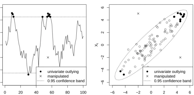
Approaches based on univariate transformations ignore the serial dependence of the data, possibly downweight good observations and overlook outliers. The left panel of Figure 1 depicts a realization of an AR process with φ0 = 0 andφ1 = 0.9. Prediction bounds based

(11)

0 20 40 60 80 100 −6 −4 −2 0 2 4 6 ●● ● ● ● ● ● ●●_● ● _{univariate outlying} manipulated 0.95 confidence band t Xt ● ● ● ● ● ● ● ● _● ● ● ● ● ● ● ● ● ● ● ● ● ● ● ● ● ● ● ● ● ● ● ● ● ● ● ● ● ● ● ● ● ● ● ● ● ● ● ● ● ● ● ● ● ● ● ● ● ● ● ● ● ● ● ● ● ● ● ● ● ● ● ● ● ● ● ● ● ● ● ● ●● ● ● ● ● ● ● ● ● ● ● ● ● ● ● ● ● ● −6 −4 −2 0 2 4 6 −6 −4 −2 0 2 4 6 ● _● ● ● ●● ● ● ● ● ● ● ● ● ● ● ● ● ● ● ● _{univariate outlying} manipulated 0.95 confidence band Xt−1 Xt

Figure 1: Time series with 95% prediction bounds based on the univariate (left) and the bivariate (right) marginal distribution corresponding to subsequent observations. Univariate margins identify the most extreme observations as outliers, while multivariate inspection takes the dependencies between subsequent observations into account and identifies the true outliers.

possible outliers, although these observations might be due to the dynamics of the underlying process. A bivariate or even multivariate analysis based on the marginal distribution of subsequent observations (Gather et al., 2002) allows to take the dependencies among subsequent observations into account, and can achieve better downweighting of spurious observations in the subsequent analysis than a simple univariate consideration. Estimation of the acf from a robust estimate of the multivariate covariance matrix is thus promising. Such estimators can be based e.g. on multivariate trimming or weighting. Moreover, some multivariate robust correlation estimators even gain efficiency with increasing dimension (Taskinen et al., 2006).

Multivariate methods can be formulated in terms of the data matrix Zk in (5). Note

that centering is unnecessary, since the described approaches estimate a robust center. The computing time of most robust procedures increases exponentially in the dimension (Vakili and Schmitt, 2014), so one should choosek rather small. To simplify notation, we denote the

i-th row of Zk as M0i, so that we are in the usual multivariate case. The estimation result

will always be a valid covariance matrix and called Γˆ(k). There is a large literature on robust multivariate correlation estimation. We will concentrate on the most common proposals, but of course others could be employed as well.

An M-estimator of scatter (abbr.: Multi-M), which can be represented as a weighted least squares estimate, was introduced in Maronna (1976), see also Maronna et al. (2006). Given an initial estimator(µ,ˆ Σˆ)for expectation and covariance, robust weights are obtained

(12)

from the outlyingness of the observations as measured by the Mahalanobis distance

d2_i = (Mi−µˆ)0Σˆ−1(Mi −µˆ),i =1, . . . ,n+k. (25)

After that, the estimation is sequentially updated by

ˆ Σ= 1 n n+k X i=1 v(di)(Mi −µˆ)(Mi −µˆ)0 and µˆ = Pn+k i=1 w(di)Mi Pn+k i=1 w(di) , (26)

where w(di) and v(di) are suitable weights. Using the weight function v(d) = (k+ 1)/d2

results in Tyler’s M-estimator (abbr.: Multi-TylerM), which is a kind of minimax estimator within the elliptical model (Tyler, 1987).

The breakdown point (Hubert and Debruyne, 2009) of M-estimators cannot exceed an upper bound which decreases with increasing dimension (Maronna et al., 2006). Since the effective amount of outlying pairs in the estimation of the acf can be twice the number of outlying observations, other estimators might be preferred if one is interested in larger time lags.

The disadvantage of the decreasing breakdown point does not apply to multivariate S-estimators (Davies, 1987; Van Aelst and Rousseeuw, 2009) (abbr.: Multi-S). They are defined as ˆ Σ= arg min µ,Σ det(Σ) : 1 nw (Mi−µ) 0 Σ−1(Mi−µ) =b0 ,

where w is a bounded smooth and not increasing weight function, e.g.

w(y) = min y2 2 − y4 2c2 + y6 6c4, c2 6 ,

which corresponds up to a constant to Tukey’s biweight ψ−function (22). The constant c

determines the breakdown point, whereas b0 depends on the probability model; see Lopuhaa

(1989) for more details. An algorithm for computing this implicitly defined estimator can be found in Ruppert (1992). Although the breakdown point does not decrease with the number of dimensions, single outliers can cause a larger bias in higher dimensions (Maronna et al., 2006).

A popular robust covariance estimator is the minimum covariance determinant (abbr.: Multi-MCD) (Rousseeuw, 1985; Hubert and Debruyne, 2010). For a given constant α

between 0 and 0.5 the usual product moment covariance is calculated for the subset of proportion1−α which leads to the matrix with the smallest determinant. An approximate procedure was proposed by Rousseeuw and Driessen (1999), since finding this subset is very time consuming for largen. Larger trimming constantsαlead to more robust but less efficient estimators, with the efficiency for large α being rather low (Croux and Haesbroeck, 1999). For combining high robustness and large efficiency, often an additional reweighting step is added (abbr.: Multi-wMCD): Robust Mahalanobis distances are obtained based on an initial MCD fit, and then the ordinary covariance matrix is calculated from all observations with Mahalanobis distances not exceeding a certain quantile of the χ2-distribution. The

(13)

0.975-quantile has been recommended for this cut-off (Rousseeuw and Driessen, 1999). An asymptotically fully efficient reweighting step (abbr.: Multi-effMCD) with a data-adaptive choice of the quantile was suggested in Gervini (2003).

Multivariate outliers can be inconspicuous if one only looks at individual dimensions, but there there is always a one-dimensional projection in which the observation is outlying (Hadi et al., 2009). Based on this idea, Stahel (1981) and Donoho (1982) proposed to use the maximal distance to the median for every possible projection to measure outlyingness, i.e.

ri = max

a:kak=1

a0Mi−med(Zka)

MAD(Zka)

,

withk·kbeing the Euclidean norm. Practical algorithms only consider a finite set of randomly chosen vectors for a. The number of such directions needs to increase strongly for higher dimensions to ensure reliable outlier detection. The resulting Stahel-Donoho estimator (abbr.: Multi-SD) is defined as the weighted covariance

ˆ Σ= _P_n1 i=1wi n X i=1 wi(Mi−µˆ)(Mi−µˆ)0 and µˆ = 1 Pn i=1wi n X i=1 wiMi.

A common choice of the weight function is wi = min

1,_rc

i

2

, andcis often chosen as the 0.975-quantile of the χ2-distribution with k+ 1 degrees of freedom (Croux and Haesbroeck, 1999).

3.5. Estimation based on variances

An estimation principle for covariances and correlations based on estimators of variances has been proposed by Gnanadesikan and Kettenring (1972). In the context of autocorrelation estimation for stationary time series, the underlying formula reads

ρ(h) = Cor(Xt+h, Xt) =

Var(Xt+h+Xt)−Var(Xt+h−Xt)

Var(Xt+h+Xt) +Var(Xt+h−Xt)

, (27)

see Ma and Genton (2000). The usual correction factors necessary for making robust scale estimators consistent at a certain distribution are not needed when applying them for correlation estimation, since they cancel out if Xt+h+Xt and Xt+h−Xt are in the same

location-scale family. This is fulfilled, e.g., if Xt+h and Xt are jointly normal or, more

generally, elliptically-symmetric distributed. Note that this approach does not necessarily yield a positive-semidefinite estimation of the acf.

For estimation of the variances on the right hand side of (27), Gnanadesikan and Kettenring (1972) suggested trimmed and winsorized variances. Since any reasonable estimator of variability can be applied, Ma and Genton (2000) proposed Qn (Rousseeuw and

Croux, 1993) (abbr.: GK-Qn), because of its high asymptotical breakdown point of 0.5 and its good asymptotical efficiency of 0.82 for i.i.d. Gaussian samples. The Qn corresponds

(14)

In the context of ordinary correlation Maronna and Zamar (2002) recommended the so called τ-scale estimator (abbr.: GK-tau)

ˆ σ2(X1, . . . , Xn) = ˆ σ₀2 n n X i=1 dc2 Xi−µˆ ˆ σ0 , (28)

where µˆ is a weighted mean of the observations, σˆ0 their MAD and dc(x) = min(x2, c2).

In Maronna and Zamar (2002) tuning constants c1 = 4.5 (for µˆ) and c2 = 3 for a good

trade-off between efficiency and robustness are suggested, resulting in an asymptotic Gaussian efficiency of 0.8 in case of independent observations. The good properties of this estimator in the bivariate i.i.d. case are promising for the estimation of autocorrelations.

3.6. Estimation based on robust filtering

As mentioned above, clean observations can be outlying with respect to the marginal distribution and thus be unnecessarily downweighted by estimators based on univariate transformations, if the autocorrelations ρ(h) are large positive and slowly decaying. The robust filtering approach overcomes this problem by taking the time series structure into account. The idea is to measure the outlyingness of the prediction residuals Up,t instead of

Xt itself. After replacing outliers by reasonable values, one can either calculate the sample

acf (abbr.: Filter-acf) or use the fitted AR process and translate this into the acf via the Yule-Walker equations (abbr.: Filter-ar). Robust filtering was already introduced by Masreliez (1975), but we will stick to the filter described in Maronna et al. (2006), which is a slight modification proposed by Martin and Thomson (1982). Note that this algorithm is quite extensive so we will summarize only the main ideas and refer to Maronna et al. (2006, pp. 272–277 and 320–321) for details.

Let X˜t be centered for example by the median and approximate the process by an AR

model of order p ∈ _N. A kind of robust AIC criterion to determine p was proposed by Maronna et al. (2006). LetYt= (Yt, . . . , Yt−p)0 denote the vector of robustly filtered values

and Φ = φ1, . . . φp−1 φp Ip−1 0p−1 (29) the so called transition matrix. From this one calculates the one step ahead predictions

ˆ Xt = p X i=1 φiYt−i

and its residuals

˜

Ut=Xt−Xˆt.

Note that this is similar to usual prediction residuals defined in (15), just replacing Xj byYj

for j =t−1, . . . , t−p to make it more robust. Eventually one sets

Yt = ΦYt−1+ mt st ψ U˜t st ! , (30)

(15)

where ψ can be for example Tukey’s bisquare function (22), and st ∈ R and mt ∈ Rp are

defined recursively. Looking only at the first row of the equations in (30) we get

Yt = ˆXt+stψ ˜ Ut st ! , (31)

indicating that Yt will be close to Xt if |U˜t| is small, and close to Xˆt if it is large. Using the

vector recursion instead of a simpler one dimensional equation (31) offers the advantage that if Xt is an outlier, the algorithm will also use future information on Xs, s > t, to determine

ˆ

Xt.

Finally, we want to emphasize the importance ofst, which is a scale estimator for the residuals

˜

Ut. The reason for using a time-dependent instead of a simpler global estimation is that in

case of outliers there is a chance that the algorithm loses the datatrack afterwards. In this case st will increase and thus provide the filtered values more variation to get back to the

data more quickly. See Martin and Thomson (1982) for more details.

The parameters φ1, . . . , φp can be estimated by minimizing the variance of the prediction

residuals

ˆ

σ( ˜Up+1(φ1, . . . , φp), . . . ,U˜n(φ1, . . . , φp)). (32)

For σˆ Maronna et al. (2006) proposed the τ-scale (28) because of its quick computation and good robustness. Since a non-convex function needs to be optimized overp parameters, they suggested sequential minimization based on the Durbin-Levinson algorithm. This converts the problem intop one-dimensional optimizations, which can easily be done by a grid search. 3.7. Implementation

To the best of our knowledge implementations of robust autocorrelation estimators are scarce in statistical software packages. The robust filtering approach and the GK approach (see Ma and Genton, 2000) have been implemented in S-Plus. Implementation of the estimation procedures is straightforward at least for the approaches which are based on two-or multidimensional ctwo-orrelation estimattwo-ors, since these estimattwo-ors are readily available in R (R Core Team, 2012).

The multivariate S, Stahel-Donoho and MCD correlation estimators are available in the

rrcov package (Todorov and Filzmoser, 2009). For Tyler’s multivariate M-estimator the

ICSNP package (Nordhausen et al., 2012) can be used, whereas a multivariate M-estimator

is available in the SpatialNP package (Sirkia et al., 2012). Both use the sample mean and covariance as initial estimators. The M-estimator uses the Huber weights w(di) =

min(1, co/|di|) = v(di)r, which correspond to (21) with co =

p

F−1₍₀_.₉₎ _{being the square}

root of the 90% percentile of theχ2_{-distribution with}_k_{+ 1}_{degrees of freedom. The parameter}

r depends on co and ensures consistency under normality. For the S-estimator c is chosen

such that the optimal breakdown point of 0.5 is achieved.

For the data-adaptively reweighted MCD we use the conventionally weighted MCD as a start estimator, resulting therefore in a two step reweigthing procedure for the raw MCD.

(16)

For Masarotto’s approach we choose the median and Qn as initial estimators for location

and spread of the time series. Robust scale estimators like the τ-scale and Qn can be found

in the package robustbase (Rousseeuw et al., 2014).

We use an own implementation of the robust filtering approach. For translating the estimatedφˆi into the acf we apply (18) instead of (11), fitting AR models of increasing order,

since it produces more stable results. For optimization of (32) we use the functionoptimize, which is based on the ALGOL localmin procedure (for details see Brent, 1973, pp. 72–80). We noticed in our simulations that this algorithm yields comparable results but needs only a fraction of the computation time of the proposed grid search.

We have already mentioned the importance of bias reducing transformations for estimators based on univariate transformations. We approximate these under the assumption of bivariate i.i.d. normal data, see Chakhchoukh (2010). Note that this transformation is independent of the time series model. Based on 10 000 runs withn = 100observations each we calculate the average estimated correlation for correlation coefficientsρ varying on a fine grid between -1 and 1. The transformation is approximated by the inverse of the linear interpolation of these averages. Like for the transformations of Kendall’s τ and Spearman’s ρthe result is biased for small sample sizes n, but for increasing n and normally distributed innovations this bias will vanish.

3.8. Positive-semidefiniteness

From the above approaches the usual sample acf, the procedures using partial autocorre-lations, the acf of the robustly filtered values as well as the Gaussian rank autocorrelation are guaranteed to be positive-semidefinite.

Bivariate correlation estimators do not necessarily yield positive-definite correlation matrices unless they calculate the usual correlation based on transformed data. A further problem arises for multivariate correlation estimators, resulting in positive-semidefinite matrices which do not possess a Toeplitz structure, meaning that there will be different values on the off-diagonals. Enforcing this by averaging the off-diagonals, for instance, can destroy the positive-semidefiniteness. Construction of the empirical counterpart of the correlation matrix Ξ(k) _{defined in formula (7) allows to apply transformations which achieve}

positive-semidefiniteness, but this destroys the Toeplitz structure.

A more appealing approach is finding the best positive-semidefinite Toeplitz approximation, minimizing e.g. the Frobenius norm (Al-Homidan, 2006). In our simulations we use the simple projection method proposed there, which can be described as follows. LetA be any real symmetric matrix, in our case Ξˆ(k), and A =U DU0 denote an eigenvalue decomposition, where D is a diagonal matrix containing all eigenvalues. If A is not positive-semidefinite there will be some eigenvalues smaller than zero. Setting these to zero yields the matrix D˜

and results in a projection Pp(A) =UDU˜ 0, which is positive-semidefinite but not Toeplitz.

Furthermore, denote byPt(A)the matrix which results from setting all off-diagonal elements

of order j to its average for j = 1, . . . k−1. These projections can be iterated until the change in the Frobenius norm becomes negligible.

(17)

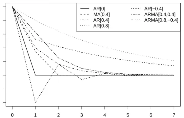
Abbr. AR[0] AR[0.4] AR[0.8] AR[-0.4] MA[0.4] ARMA[0.4,0.4] ARMA[0.8,-0.4]

φ1 0 0.4 0.8 -0.4 0 0.4 0.8

θ1 0 0 0 0 0.4 0.4 -0.4

Table 1: Considered processes and their abbreviations.

0 1 2 3 4 5 6 7 −0.4 −0.2 0.0 0.2 0.4 0.6 0.8 1.0 AR[0] MA[0.4] AR[0.4] AR[0.8] AR[−0.4] ARMA[0.4,0.4] ARMA[0.8,−0.4] Theoretical acf Lag

Figure 2: Autocorrelation functions of the processes considered in the simulations.

4. Simulation

There are not many theoretical results available for comparing the different autocorrelation estimators. We thus perform a simulation study using the statistical software R (R Core Team, 2012) with the functions and tuning constants mentioned when introducing the different estimators. The simulation code is available from the authors upon request. We restrict ourselves to first order autoregressive moving average (ARMA) processes because of their simplicity and popularity, considering the seven parameter settings shown in Table 1 along with their abbreviations. Figure 2 indicates that this selection covers rather different autocorrelation functions. If not explicitly stated otherwise, the innovations are standard normal.

We calculate the acf only for the first seven lags for different reasons. Multivariate correlation estimators are time consuming for large lags and the acf of most of the processes is nearly zero for lags larger than six. So we do not expect qualitatively different behavior for

(18)

higher time lags. However, simulations indicate a slight loss of efficiency of robust estimators for higher time lags.

To simplify the comparison we consider maximal bias and minimal efficiency across all lags instead of looking at all seven time lags separately. Simulations reveal that the maximal (absolute) bias

max

h=1,...,7|Bias( ˆρ(h))|

is usually realized for h= 1, whereas the minimal efficiency compared to the sample acf ρ˜ min

h=1,...,7(MSE( ˜ρ(h))/MSE( ˆρ(h)))

occurs often for h= 1 or the largest lag considered here, h= 7. In the case of contaminated data, we calculate the efficiency relative to the sample acf for clean data. This measures the amount of information lost due to outliers when using a robust estimator.

4.1. Efficiency for uncontaminated data

First we investigate the properties in case of clean data without outliers, starting with the AR[0.4] model. The results are based on 10 000 runs each. As mentioned before the empirical acf is biased for smalln. As can be seen in Figure 3, the small sample bias is comparable to the robust alternatives. The bias is usually negative, except for the robust filtering approach and the PA-Quadrant. Tyler’s M-estimator and RA-estimators are less biased than the other methods for smalln, resulting in a good finite sample efficiency. Generally, multivariate S-and M-estimators achieve high efficiencies. GK, rank S-and sign based approaches S-and also the reweighted MCD versions need larger samples to get a small MSE.

The findings for other models are similar. For processes with strong positive autocorrela-tions the maximal bias increases for all estimators just as the minimal efficiency. Nevertheless, the order of the estimators with respect to efficiency nearly stays the same.

In time series we often face distributions with tails heavier than the Gaussian (Davis and Resnick, 1986; Loretan and Phillips, 1994; Politis, 2009; Rojo, 2013). Estimators should remain reliable in case of such departures from normality. Therefore we considered maximal absolute bias and minimal efficiency for AR models with t-distributed innovations of different degrees of freedom. Already for three degrees of freedom the results were similar to those under normality. Only estimators based on partial autocorrelation considerably lose efficiency. Note that three degrees of freedom corresponds to the heaviest tails possible, for which the acf is defined under t-distributions. Simulations agree with the theoretical result that the sample acf of a linear process is still√n-consistent without the need of fourth moments, see Davis and Mikosch (1998).

4.2. Robustness under contamination

Additive outliers are known to be particularly harmful for the estimation of dependence parameters. Such outliers describe e.g. measurement errors, where a certain valueω is added to the observation at time t, t = 1, . . . , n, see Fox (1972). While for the empirical acf the effect of an outlier increases in ω due to monotonicity, for robust estimators this influence is

(19)

MSE−efficiency Filter−ar Filter−acf Mediancor Trim RA−Tukey RA−Huber PA−M PA−Quadrant PA−Spearman PA−Kendall Quadrant Spearman Kendall GRCor Multi−TylerM Multi−M Multi−S Multi−SD Multi−effMCD Multi−wMCD Multi−rMCD GK−tau GK−Qn emp. acf 0.1 0.05 0 0 0.2 0.4 0.6 0.8 1

Maximal absolute bias

Figure 3: Efficiency (left) and bias (right) forn = 50, 100, 500(from top to bottom in each panel) for AR[0.4] with normal innovations.

(20)

0 2 4 6 8 10 0.0 0.2 0.4 0.6 0.8 emp. acf Spearman GK−Qn RA−Tukey Filter−acf Multi−S ω Bias 0 2 4 6 8 10 0.0 0.2 0.4 0.6 0.8 ω Bias

Figure 4: Simulated bias of a contaminated AR[0] model withn= 100and a patch of 5 (left) or 20 outliers (right).

generally bounded. However, while the influence is still monotone inωfor rank-based or other monotone estimators, it can even decrease for very large values ofω for other estimators, e.g. for so called redescenders like S-estimators, see Figure 4. This means that different outlier sizes are worst-case for different estimators, so that it is not fair to consider only a single value of ω, which is identical for all estimators. Therefore we simulate maximal absolute bias and minimal efficiency for different outlier sizesω ∈ {ω0

p

γ(0) :ω0 = 2,2.5, . . . ,5,6, . . . ,10},

which are proportional to the marginal standard deviation, and choose the worst results for each estimator.

Furthermore, we contaminate an increasing number n0 ∈ {5,10,15,20,25} of values of

the original time series of lengthn= 100to see how many outliers an estimator can deal with. As mentioned before, robust estimators cannot be expected to cope with more than 25% contaminated observations in our context, so it is not reasonable to choosen0 larger than

25. Moreover, we consider both isolated and patchy outliers, since these will have different effects. All results are based on 1000 simulation runs.

We first treat the situation of isolated outliers, which drive the sample acf towards zero. The positions of the outliers are sampled randomly for each time series. We show the results for the AR[0.8] model first. As one can see in Figure 5, the empirical acf becomes useless already forn0 = 5outliers. In the same situation, some robust alternatives lose more than

half of their efficiency, even though they are rarely more biased. Estimators which cope with additive outliers well are the ones based on robust filtering and to some extent also the GK approaches and the multivariate SD.

The estimators generally behave better for the other models. This is not surprising, since the bias effect is more limited there. Recall that the AR[0.8] model is the one with the largest

(21)

Figure 5: Efficiency (left) and bias (right) for a contaminated AR[0.8] model with n = 100 and n0 =

(22)

absolute correlations considered here. In models with rather small autocorrelations other robust estimators like RA and GK approaches outperform the Filter-acf, which seems to behave especially well if the autocorrelations are strongly positive.

Patchy (consecutive) outliers increase the sample acf at small time lags towards one. The position of the contaminated values was set to {51, . . . ,50 +n0} in a time series of length

100. We first look at the AR[0]-model. Again the estimation by the empirical acf is already useless for n0 = 5 outliers, see Figure 6. Robust estimators can cope with this situation

much better and rarely lose more than the half of their efficiency. Estimators based on SD and MCD and to some extent also the multivariate S-estimator perform quite well. Even for large amounts of outliers they are little biased and lose only little efficiency. Different kinds of reweighting which boost efficiency under the clean model do not significantly increase the bias or vulnerability to outliers and should be preferred.

The estimators generally behave better for the other models, except for the AR[-0.4]. Recall that the AR[0] and AR[-0.4] are the processes with the smallest autocorrelations, hence patchy outliers cause the largest bias there. For models with large autocorrelations a small number of consecutive outliers even improves the estimation by canceling the small sample bias. Rank and RA-estimators perform very well for these models.

4.3. Positive-semidefiniteness

We have mentioned the problem of positive-semidefiniteness repeatedly. Our simulations reveal that this is mainly a problem of little efficient estimators like quadrant correlation and the 50% trimming (median) approach. We never noticed problems for multivariate approaches except for the raw MCD, which occasionally produces indefinite estimations if the model is close to being non-stationary. It turns out that consistency corrections for the approaches based on univariate transformations often destroy definiteness. Whereas the difference between the original estimation and the enforced positive-semidefinite one is negligible for the RA-estimators, we observed changes up to 0.08 for trimmed and median based correlation. There can be even greater discrepancies for the Filter-AR estimator, which might be caused by some instability of our implementation of this procedure. We rarely noticed indefinite estimations by the variance based approaches. Enforcing positive-semidefiniteness increases the efficiency of trimmed estimators slightly.

5. Conclusion

Some of the proposals for robust autocorrelation estimation are borrowed from the usual correlation estimation applied to all pairs of observations (Xt, Xt+h) at a certain time lag h,

with the intention that good robustness properties and high efficiency under normality carry over to the time series context. A problem arising in this context is that every outlier can enter two pairs of observations, so that the number of contaminated pairs can be up to twice the number of outliers.

Our simulation study confirms that even a small fraction of contamination can make the empirical acf useless. The robust filter algorithm yields good results even in case of many isolated outliers. Estimation based on a reweighted MCD is favorable, if there are

(23)

Figure 6: Efficiency under an outlier patch of lengthn0 = 0,5,10,15,20,25(from top to bottom in each

(24)

patchy outliers. A good compromise represents the approach based on the Stahel-Donoho estimator, but it is computationally demanding. If one looks for a relatively quick estimator the approach based on robust variances seems to be a good choice, since they also generally yield good results. A possible lack of positive-semidefiniteness can easily be fixed by a projection algorithm.

It needs to be kept in mind that in the simulations reported here we focus on the case of innovations from a contaminated Gaussian or at least continuous-symmetric distribution. Results look different e.g. for count time series as reported in Fried et al. (2014), where rank based estimators performed rather well.

Acknowledgements

The financial support of the Deutsche Forschungsgemeinschaft (SFB 823, “Statistical modelling of nonlinear dynamic processes”) is gratefully acknowledged.

References

Al-Homidan, S. (2006). Semidefinite and second-order cone optimization approach for the toeplitz matrix approximation problem. Journal of Numerical Mathematics, 14(1):1–15.

Boudt, K., Cornelissen, J., and Croux, C. (2012). The gaussian rank correlation estimator: robustness properties. Statistics and Computing, 22(2):471–483.

Box, G. E. P., Jenkins, G. M., and Reinsel, G. C. (1994). Time series analysis: forecasting and control. Prentice Hall, Englewood Cliff, N.J., 3rd edition.

Brent, R. P. (1973). Algorithms for minimization without derivatives. Prentice-Hall, Englewood Cliffs, N.J. Brockwell, P. and Davis, R. A. (2006). Time series: theory and methods. Springer, New York, 2nd edition. Brockwell, P. J. (2009). Autocovariance. Wiley Interdisciplinary Reviews: Computational Statistics, 1(2):187–

198.

Brockwell, P. J. (2011). Autoregressive processes. Wiley Interdisciplinary Reviews: Computational Statistics, 3(4):316–331.

Bustos, O. H. and Yohai, V. J. (1986). Robust estimates for ARMA models. Journal of the American Statistical Association, 81(393):155–168.

Caiado, J., Crato, N., and Peña, D. (2006). A periodogram-based metric for time series classification.

Computational Statistics & Data Analysis, 50(10):2668–2684.

Chakhchoukh, Y. (2010). A new robust estimation method for ARMA models. IEEE Transactions on Signal Processing, 58(7):3512–3522.

Chan, W.-S. (1992). A note on time series model specification in the presence of outliers. Journal of Applied Statistics, 19(1):117–124.

Chan, W.-S. and Wei, W. W. (1992). A comparison of some estimators of time series autocorrelations.

Computational statistics & data analysis, 14(2):149–163.

Croux, C. and Dehon, C. (2010). Influence functions of the spearman and kendall correlation measures.

Statistical Methods & Applications, 19(4):497–515.

Croux, C. and Haesbroeck, G. (1999). Influence function and efficiency of the minimum covariance determinant scatter matrix estimator. Journal of Multivariate Analysis, 71(2):161–190.

Davies, P. (1987). Asymptotic behaviour of S-estimates of multivariate location parameters and dispersion matrices. The Annals of Statistics, 15(3):1269–1292.

Davis, R. and Resnick, S. (1986). Limit theory for the sample covariance and correlation functions of moving averages. The Annals of Statistics, 14(2):533–558.

Davis, R. A. and Mikosch, T. (1998). The sample autocorrelations of heavy-tailed processes with applications to ARCH. The Annals of Statistics, 26(5):2049–2080.

(25)

Deutsch, S. J., Richards, J. E., and Swain, J. J. (1990). Effects of a single outlier on ARMA identification.

Communications in Statistics: Theory and Methods, 19(6):2207–2227.

Donoho, D. L. (1982). Breakdown properties of multivariate location estimators. Technical report, Harvard University, Boston.

Ferretti, N. E., Kelmansky, D. M., and Yohai, V. J. (1991). Estimators based on ranks for ARMA models.

Communications in Statistics – Theory and Methods, 20(12):3879–3907.

Fox, A. J. (1972). Outliers in time series. Journal of the Royal Statistical Society. Series B (Methodological), 34(3):350–363.

Fried, R., Liboschik, T., Elsaied, H., Kitromilidou, S., and Fokianos, K. (2014). On outliers and interventions in count time series following GLMs. Austrian Journal of Statistics. In press.

Garel, B. and Hallin, M. (1999). Rank-based autoregressive order identification. Journal of the American Statistical Association, 94(448):1357–1371.

Gather, U., Bauer, M., and Fried, R. (2002). The identification of multiple outliers in online monitoring data.

Estadistica, 54:289–338.

Gervini, D. (2003). A robust and efficient adaptive reweighted estimator of multivariate location and scatter.

Journal of Multivariate Analysis, 84(1):116–144.

Gnanadesikan, R. and Kettenring, J. R. (1972). Robust estimates, residuals, and outlier detection with multiresponse data. Biometrika, 28(1):81–124.

Hadi, A. S., Imon, A., and Werner, M. (2009). Detection of outliers. Wiley Interdisciplinary Reviews: Computational Statistics, 1(1):57–70.

Hubert, M. and Debruyne, M. (2009). Breakdown value. Wiley Interdisciplinary Reviews: Computational Statistics, 1(3):296–302.

Hubert, M. and Debruyne, M. (2010). Minimum covariance determinant. Wiley Interdisciplinary Reviews: Computational Statistics, 2(1):36–43.

Lopuhaa, H. P. (1989). On the relation between S-estimators and M-estimators of multivariate location and covariance. The Annals of Statistics, 17(4):1662–1683.

Loretan, M. and Phillips, P. C. (1994). Testing the covariance stationarity of heavy-tailed time series: An overview of the theory with applications to several financial datasets. Journal of empirical finance, 1(2):211–248.

Ma, Y. and Genton, M. G. (2000). Highly robust estimation of the autocovariance function. Journal of time series analysis, 21(6):663–684.

Makhoul, J. (1981). Lattice methods in spectral estimation. Applied Time Series Analysis, 2:301–326. Maronna, R. A. (1976). Robust M-estimators of multivariate location and scatter. The Annals of Statistics,

4(1):51–67.

Maronna, R. A., Martin, R. D., and Yohai, V. J. (2006). Robust statistics. J. Wiley, Chichester.

Maronna, R. A. and Zamar, R. H. (2002). Robust estimates of location and dispersion for high-dimensional datasets. Technometrics, 44(4):307–317.

Martin, R. D. and Thomson, D. J. (1982). Robust-resistant spectrum estimation. Proceedings of the IEEE, 70(9):1097–1115.

Masarotto, G. (1987). Robust identification of autoregressive moving average models. Applied statistics, 36(2):214–220.

Masreliez, C. (1975). Approximate non-gaussian filtering with linear state and observation relations. IEEE Transactions on Automatic Control, 20(1):107–110.

Morgenthaler, S. (2011). Robustness. Wiley Interdisciplinary Reviews: Computational Statistics, 3(2):85–94. Mottonen, J., Koivunen, V., and Oja, H. (1999). Robust autocovariance estimation based on sign and rank correlation coefficients. InProceedings of the IEEE Signal Processing Workshop on Higher-Order Statistics, pages 187–190. IEEE.

Nordhausen, K., Sirkia, S., Oja, H., and Tyler, D. E. (2012). ICSNP: Tools for Multivariate Nonparametrics. R package version 1.0-9.

Politis, D. N. (2009). Financial time series. Wiley Interdisciplinary Reviews: Computational Statistics, 1(2):157–166.

(26)

R Core Team (2012). R: A Language and Environment for Statistical Computing. R Foundation for Statistical Computing, Vienna, Austria.

Ramsey, F. L. (1974). Characterization of the partial autocorrelation function. The Annals of Statistics, 2(6):1296–1301.

Rojo, J. (2013). Heavy-tailed densities.Wiley Interdisciplinary Reviews: Computational Statistics, 5(1):30–40. Rousseeuw, P., Croux, C., Todorov, V., Ruckstuhl, A., Salibian-Barrera, M., Verbeke, T., Koller, M., and

Maechler, M. (2014). robustbase: Basic Robust Statistics. R package version 0.90-2.

Rousseeuw, P. J. (1985). Multivariate estimation with high breakdown point. Mathematical Statistics and Applications Vol. B, pages 283–297.

Rousseeuw, P. J. and Croux, C. (1993). Alternatives to the median absolute deviation. Journal of the American Statistical Association, 88(424):1273–1283.

Rousseeuw, P. J. and Driessen, K. V. (1999). A fast algorithm for the minimum covariance determinant estimator. Technometrics, 41(3):212–223.

Ruppert, D. (1992). Computing S-estimators for regression and multivariate location/dispersion. Journal of Computational and Graphical Statistics, 1(3):253–270.

Schlittgen, R. and Streitberg, B. H. J. (2001). Zeitreihenanalyse. Oldenbourg, München.

Sirkia, S., Miettinen, J., Nordhausen, K., Oja, H., and Taskinen, S. (2012). SpatialNP: Multivariate nonparametric methods based on spatial signs and ranks. R package version 1.1-0.

Stahel, W. (1981). Robust estimation: Infinitesimal optimality and covariance matrix estimators. PhD thesis, ETH, Zurich, Switzerland.

Taskinen, S., Croux, C., Kankainen, A., Ollila, E., and Oja, H. (2006). Influence functions and efficiencies of the canonical correlation and vector estimates based on scatter and shape matrices.Journal of Multivariate Analysis, 97(2):359–384.

Todorov, V. and Filzmoser, P. (2009). An object-oriented framework for robust multivariate analysis.Journal of Statistical Software, 32(3):1–47.

Tyler, D. E. (1987). A distribution-free M-estimator of multivariate scatter. The Annals of Statistics, 15(1):234–251.

Vakili, K. and Schmitt, E. (2014). Finding multivariate outliers with fastPCS. Computational Statistics & Data Analysis, 69:54–66.

Van Aelst, S. and Rousseeuw, P. (2009). Minimum volume ellipsoid. Wiley Interdisciplinary Reviews: Computational Statistics, 1(1):71–82.

Vecchia, A. and Ballerini, R. (1991). Testing for periodic autocorrelations in seasonal time series data.

Biometrika, 78(1):53–63.

Wei, W. W. (1990). Time series analysis: Univariate and Multivariate Methods. Addison-Wesley, Redwood City.

(27)

(28)