Noname manuscript No.
(will be inserted by the editor)
Incremental Eigenpair Computation for Graph Laplacian
Matrices: Theory and Applications
?Pin-Yu Chen · Baichuan Zhang · Mohammad Al Hasan
the date of receipt and acceptance should be inserted later
Abstract The smallest eigenvalues and the associated eigenvectors (i.e., eigen-pairs) of a graph Laplacian matrix have been widely used in spectral clustering and community detection. However, in real-life applications the number of clus-ters or communities (say,K) is generally unknown a-priori. Consequently, the majority of the existing methods either chooseK heuristically or they repeat the clustering method with different choices ofKand accept the best clustering result. The first option, more often, yields suboptimal result, while the second option is computationally expensive. In this work, we propose an incremental method for constructing the eigenspectrum of the graph Laplacian matrix. This method leverages the eigenstructure of graph Laplacian matrix to obtain the K-th smallest eigenpair of the Laplacian matrix given a collection of all previously computedK−1 smallest eigenpairs. Our proposed method adapts the Laplacian matrix such that the batch eigenvalue decomposition problem transforms into an efficient sequential leading eigenpair computation problem. As a practical application, we consider user-guided spectral clustering. Specif-ically, we demonstrate that users can utilize the proposed incremental method for effective eigenpair computation and for determining the desired number of clusters based on multiple clustering metrics.
Keywords Graph Mining and Analysis, Graph Laplacian, Incremental Eigenpair Computation, User-Guided Spectral Clustering
? This manuscript is an extended version of a paper that was presented at ACM KDD
Workshop on Mining and Learning with Graphs (MLG 2016) [14]. Pin-Yu Chen
AI Foundations - Learning Group, IBM Thomas J. Watson Research Center E-mail:{[email protected]}
Baichuan Zhang
Purdue University, West Lafayette E-mail:{[email protected]}
Mohammad Al Hasan
Indiana University Purdue University Indianapolis E-mail:{[email protected]}
___________________________________________________________________ This is the author's manuscript of the article published in final edited form as:
Chen, P.-Y., Zhang, B., & Hasan, M. A. (2018). Incremental eigenpair computation for graph Laplacian matrices: theory and applications. Social Network Analysis and Mining, 8(1), 4. https://doi.org/10.1007/s13278-017-0481-y
1 Introduction
Over the past two decades, the graph Laplacian matrix and its variants have been widely adopted for solving various research tasks, including graph par-titioning [42], data clustering [5, 32, 56], community detection [7, 13, 50], con-sensus in networks [37, 53], accelerated distributed optimization [29], dimen-sionality reduction [2, 52], entity disambiguation [46, 60–64], link prediction [15, 19, 20, 59], graph signal processing [12, 48], centrality measures for graph connectivity [6], multi-layer network analysis [11, 30], interconnected physical systems [43], network vulnerability assessment [9], image segmentation [18,47], gene expression [28,31,39], among others. The fundamental task is to represent the data of interest as a graph for analysis, where a node represents an entity (e.g., a pixel in an image or a user in an online social network) and an edge represents similarity between two multivariate data samples or actual relation (e.g., friendship) between nodes [32]. More often the K eigenvectors associ-ated with the K smallest eigenvalues of the graph Laplacian matrix are used to cluster the entities intoKclusters of high similarity. For brevity, throughout this paper we will call these eigenvectors as theKsmallest eigenvectors.
The success of graph Laplacian matrix based methods for graph parti-tioning and spectral clustering can be explained by the fact that acquiring K smallest eigenvectors is equivalent to solving a relaxed graph cut mini-mization problem, which partitions a graph into K clusters by minimizing various objective functions including min cut, ratio cut or normalized cut [32]. Generally, in clustering the value K is selected to be much smaller than n (the number of data points), making full eigen decomposition (such as QR decomposition) unnecessary. An efficient alternative is to use methods that are based on power iteration, such as Arnoldi method or Lanczos method, which computes the leading eigenpairs through repeated matrix vector multi-plication [54, 55]. ARPACK [27] library is a popular parallel implementation of different variants of Arnoldi and Lanczos methods, which is used by many commercial software including Matlab.
However, in most situations the best value ofKis unknown and a heuristic is used by clustering algorithms to determine the number of clusters, e.g., fixing a maximum number of clustersKmax and detecting a large gap in the values of theKmax largest sorted eigenvalues or normalized cut score [34, 40]. Alter-natively, this value ofK can be determined based on domain knowledge [1]. For example, a user may require that the largest cluster size be no more than 10% of the total number of nodes or that the total inter-cluster edge weight be no greater than a certain amount. In these cases, the desired choice ofK cannot be determineda priori. Over-estimation of the upper boundKmax on the number of clusters is expensive as the cost of findingK eigenpairs using the power iteration method grows rapidly withK. On the other hand, choos-ing an insufficiently large value forKmax runs the risk of severe bias. Setting Kmax to the number of data pointsn is generally computationally infeasible, even for a moderate-sized graph. Therefore, an incremental eigenpair compu-tation method that effectively computes theK-th smallest eigenpair of graph
Laplacian matrix by utilizing the previously computedK−1 smallest eigen-pairs is needed. Such an iterative method obviates the need to set an upper bound Kmax on K, and its efficiency can be explained by the adaptivity to increments inK.
By exploiting the special matrix properties and graph characteristics of a graph Laplacian matrix, we propose an efficient method for computing the (K+1)-th eigenpair given all of theKsmallest eigenpairs, which we call the In-cremental method of Increasing Orders (InIn-cremental-IO). For each increment, given the previously computed smallest eigenpairs, we show that computing the next smallest eigenpair is equivalent to computing a leading eigenpair of a particular matrix, which transforms potentially tedious numerical computa-tion (such as the iterative tridiagonalizacomputa-tion and eigen-decomposicomputa-tion steps in the Lanczos algorithm [25]) to simple matrix power iterations of known com-putational efficiency [24]. Specifically, we show that Incremental-IO can be im-plemented via power iterations, and analyze its computational complexity and data storage requirements. We then compare the performance of Incremental-IO with a batch computation method which computes all of the K smallest eigenpairs in a single batch, and an incremental method adapted from the Lanczos algorithm, which we call the Lanczos method of Increasing Orders (Lanczos-IO). For a given number of eigenpairsKiterative matrix-vector mul-tiplication of Lanczos procedure yields a set of Lanczos vectors (Q`), and a
tridiagonal matrix (T`), followed by a full eigen-decomposition of T` (` is a
value much smaller than the matrix size). Lanczos-IO saves the Lanczos vec-tors that were obtained whileK eigenpairs were computed and used those to generate new Lanczos vectors for computing the (K+ 1)-th eigenpair.
Comparing to the batch method, our experimental results show that for a given orderK, Incremental-IO provides a significant reduction in computa-tion time. Also, asKincreases, the gap between Incremental-IO and the batch approach widens, providing an order of magnitude speed-up. Experiments on real-life datasets show that the performance of Lanczos-IO is overly sensitive to the selection of augmented Lanczos vectors, a parameter that cannot be optimized a priori—for some of our experimental datasets, Lanczos-IO per-forms even worse than the batch method (see Sec. 6). Moreover, Lanczos-IO consumes significant amount of memory as it has to save the Lanczos vectors (Q`) for making the incremental approach realizable. In summary,
Lanczos-IO, although an incremental eigenpair computation algorithm, falls short in terms of robustness.
To illustrate the real-life utility of incremental eigenpair computation meth-ods, we design a user-guided spectral clustering algorithm which uses Incremental-IO. The algorithm provides clustering solution for a sequence of K values efficiently, and thus enable a user to compare these clustering solutions for facilitating the selection of the most appropriate clustering.
The contributions of this paper are summarized as follows:
1. We propose an incremental eigenpair computation method (Incremental-IO) for both unnormalized and normalized graph Laplacian matrices, by transforming the original eigenvalue decomposition problem into an effi-cient sequential leading eigenpair computation problem. Specifically, Incremental-IO can be implemented via power iterations, which possess efficient compu-tational complexity and data storage. Simulation results show that Incremental-IO generates the desired eigenpair accurately and has superior performance over the batch computation method in terms of computation time. 2. We show that Incremental-IO is robust in comparison to Lanczos-IO, which
is an incremental eigenpair method that we design by adapting the Lanczos method.
3. We use several real-life datasets to demonstrate the utility of Incremental-IO. Specifically, we show that Incremental-IO is suitable for user-guided spectral clustering which provides a sequence of clustering results for unit increment of the numberKof clusters, and updates the associated cluster evaluation metrics for helping a user in decision making.
2 Related Work
2.1 Incremental eigenvalue decomposition
The proposed method (Incremental-IO) aims to incrementally compute the smallest eigenpair of a given graph Laplacian matrix. There are several works that are named as incremental eigenvalue decomposition methods [17, 22, 35, 36, 44]. However, these works focus on updating the eigenstructure of graph Laplacian matrix of dynamic graphs when nodes (data samples) or edges are inserted or deleted from the graph, which are fundamentally different from in-cremental computation of eigenpairs of increasing orders. Consequently, albeit similarity in research topics, they are two distinct sets of problems and cannot be directly compared.
2.2 Cluster Count Selection for Spectral Clustering
Many spectral clustering algorithms utilize the eigenstructure of graph Lapla-cian matrix for selecting number of clusters. In [40], a valueKthat maximizes the gap between theK-th and the (K+ 1)-th smallest eigenvalue is selected as the number of clusters. In [34], a valueK that minimizes the sum of cluster-wise Euclidean distance between each data point and the centroid obtained from K-means clustering onKsmallest eigenvectors is selected as the number of clusters. In [58], the smallest eigenvectors of normalized graph Laplacian matrix are rotated to find the best alignment that reflects the true clusters. A model based method for determining the number of clusters is proposed in [41]. In [10], a model order selection criterion for identifying the number
of clusters is proposed by estimating the interconnectivity of the graph us-ing the eigenpairs of the graph Laplacian matrix. In [49], the clusters are identified via random walk on graphs. In [3], an iterative greedy modularity maximization approach is proposed for clustering. In [23, 45], the eigenpairs of the nonbacktracking matrix are used to identify clusters. Note that aforemen-tioned methods use only one single clustering metric to determine the number of clusters and often implicitly assume an upper bound onK(namelyKmax). As demonstrated in Sec. 6, the proposed incremental eigenpair computation method (Incremental-IO) can be used to efficiently provide a sequence of clus-tering results for unit increment of the numberK of clusters and updates the associated (potentially multiple) cluster evaluation metrics.
3 Incremental Eigenpair Computation for Graph Laplacian Matrices
3.1 Background
Throughout this paper bold uppercase letters (e.g., X) denote matrices and
Xij (or [X]ij) denotes the entry ini-th row and j-th column ofX, bold
low-ercase letters (e.g., x or xi) denote column vectors, (·)T denotes matrix or
vector transpose, italic letters (e.g., xor xi) denote scalars, and calligraphic
uppercase letters (e.g.,X orXi) denote sets. Then×1 vector of ones (zeros) is
denoted by1n (0n). The matrixIdenotes an identity matrix and the matrix
Odenotes the matrix of zeros.
We use twon×nsymmetric matrices,AandW, to denote the adjacency and weight matrices of an undirected weighted simple graphGwith nnodes andmedges.Aij = 1 if there is an edge between nodesi andj, andAij = 0
otherwise.Wis a nonnegative symmetric matrix such thatWij≥0 ifAij = 1
and Wij = 0 if Aij = 0. Letsi = Pn
j=1Wij denote the strength of node i.
Note that when W= A, the strength of a node is equivalent to its degree.
S= diag(s1, s2, . . . , sn) is a diagonal matrix with nodal strength on its main
diagonal and the off-diagonal entries being zero.
The (unnormalized) graph Laplacian matrix is defined as
L=S−W. (1)
One popular variant of the graph Laplacian matrix is the normalized graph Laplacian matrix defined as
LN =S− 1 2LS− 1 2 =I−S− 1 2WS− 1 2, (2) where S−12 = diag(√1 s1, 1 √ s2, . . . , 1 √
sn). The i-th smallest eigenvalue and its associated unit-norm eigenvector of L are denoted by λi(L) and vi(L),
re-spectively. That is, the eigenpair (λi,vi) of L has the relation Lvi = λivi,
and λ1(L) ≤ λ2(L) ≤ . . . ≤ λn(L). The eigenvectors have unit Euclidean
Table 1: Utility of the established lemmas, corollaries, and theorems. Graph Type / Graph Laplacian Matrix Unnormalized Normalized
Connected Graphs Lemma1,Theorem1 Corollary1,Corollary3 Disconnected Graphs Lemma2,Theorem2 Corollary2,Corollary4
and vT
i vj = 0 if i 6= j. The eigenvalues of L are said to be distinct if
λ1(L)< λ2(L)< . . . < λn(L). Similar notations are used forLN.
3.2 Theoretical foundations of the proposed method (Incremental-IO)
The following lemmas and corollaries provide the cornerstone for establishing the proposed incremental eigenpair computation method (Incremental-IO). The main idea is that we utilize the eigenspace structure of graph Laplacian matrix to inflate specific eigenpairs via a particular perturbation matrix, with-out affecting other eigenpairs. Incremental-IO can be viewed as a specialized Hotelling’s deflation method [38] designed for graph Laplacian matrices by ex-ploiting their spectral properties and associated graph characteristics. It works for both connected, and disconnected graphs using either normalized or un-normalized graph Laplacian matrix. For illustration purposes, in Table 1 we group the established lemmas, corollaries, and theorems under different graph types and different graph Laplacian matrices.
Lemma 1 Assume thatGis a connected graph and Lis the graph Laplacian
withsidenoting the sum of the entries in thei-th row of the weight matrixW.
Let s=Pni=1si and define Le=L+sn1n1Tn. Then the eigenpairs ofLe satisfy
(λi(Le),vi(Le)) = (λi+1(L),vi+1(L)) for1 ≤i≤n−1 and (λn(Le),vn(Le)) =
(s,√1n
n).
Proof Since L is a positive semidefinite (PSD) matrix [16], λi(L)≥0 for all
i. Since Gis a connected graph, by (1) L1n = (S−W)1n =0n. Therefore,
by the PSD property we have (λ1(L),v1(L)) = (0,√1n
n). Moreover, sinceL is
a symmetric real-valued square matrix, from (1) we have
trace(L) = n X i=1 Lii = n X i=1 λi(L) = n X i=1 si =s. (3)
By the PSD property of L, we have λn(L) < ssince λ2(L) >0 for any
1Tnvi(L) = 0 for all i ≥ 2) the eigenvalue decomposition of Le can be repre-sented as e L= n X i=2 λi(L)vi(L)vTi(L) + s n1n1 T n = n X i=1 λi(Le)vi(Le)vTi(Le), (4)
where (λn(Le),vn(Le)) = (s,√1nn) and (λi(Le),vi(Le)) = (λi+1(L),vi+1(L)) for 1≤i≤n−1.
Corollary 1 For a normalized graph Laplacian matrix LN, assume G is a
connected graph and letLeN =LN+2sS
1 21n1T nS 1 2. Then(λi(LeN),vi(LeN)) = (λi+1(LN),vi+1(LN))for1≤i≤n−1 and(λn(LeN),vn(LeN)) = (2,S 1 21n √ s ).
Proof Recall from (2) that LN = S−
1 2LS−
1
2, and also we have LNS 1 21n = S−12L1n = 0n. Moreover, it can be shown that 0 ≤ λ1(LN) ≤ λ2(LN) ≤
. . . ≤ λn(LN) ≤ 2 [33], and λ2(LN) > 0 if G is connected. Following the
same derivation procedure for Lemma 1 we obtain the corollary. Note that
S12 = diag(√s1,√s2, . . . ,√sn) and (S121n)TS121n=1T
nS1n =s.
Lemma 2 Assume that G is a disconnected graph with δ ≥ 2 connected
components. Let s = Pni=1si, let V = [v1(L),v2(L), . . . ,vδ(L)], and let
e
L=L+sVVT. Then(λi(Le),vi(Le)) = (λi+δ(L),vi+δ(L))for1≤i≤n−δ,
λi(Le) =sforn−δ+ 1≤i≤n, and[vn−δ+1(Le),vn−δ+2,(Le), . . . ,vn(Le)] =V.
Proof The graph Laplacian matrix of a disconnected graph consisting of δ
connected components can be represented as a matrix with diagonal block structure, where each block in the diagonal corresponds to one connected com-ponent inG[8], that is,
L= L1 O O O O L2 O O O O . .. O O O O Lδ , (5)
where Lk is the graph Laplacian matrix of k-th connected component in G.
From the proof ofLemma1 each connected component contributes to exactly one zero eigenvalue forL, and
λn(L)< δ X k=1 X i∈componentk λi(Lk) = δ X k=1 X i∈componentk si =s. (6)
Lemma1 applies to the (unnormalized) graph Laplacian matrix of a con-nected graph, and the corollary below applies to the normalized graph Lapla-cian matrix of a connected graph.
Corollary 2 For a normalized graph Laplacian matrixLN, assumeGis a
dis-connected graph withδ≥2connected components. LetVδ= [v1(LN),v2(LN),
. . . ,vδ(LN)], and letLeN =LN+2VδVTδ.Then(λi(LeN),vi(LeN)) = (λi+δ(LN),
vi+δ(LN)) for 1 ≤ i ≤ n−δ, λi(LeN) = 2 for n−δ+ 1 ≤ i ≤ n, and
[vn−δ+1(LeN),vn−δ+2,(LeN), . . . ,vn(LeN)] =Vδ.
Proof The results can be obtained by following the same derivation proof
procedure as in Lemma 2 and the fact thatλn(LN)≤2 [33].
Remark 1 note that the columns of any matrix V0 =VR with an
orthonor-mal transformation matrix R(i.e.,RTR=I) are also the largestδ
eigenvec-tors ofLe andLeN in Lemma2 and Corollary2. Without loss of generality
we consider the caseR=I.
3.3 Incremental method of increasing orders (Incremental-IO)
Given theK smallest eigenpairs of a graph Laplacian matrix, we prove that computing the (K+ 1)-th smallest eigenpair is equivalent to computing the leading eigenpair (the eigenpair with the largest eigenvalue in absolute value) of a certain perturbed matrix. The advantage of this transformation is that the leading eigenpair can be efficiently computed via matrix power iteration methods [25, 27].
LetVK = [v1(L),v2(L), . . . ,vK(L)] be the matrix with columns being the
K smallest eigenvectors ofL and letΛK = diag(s−λ1(L), s−λ2(L), . . . , s− λK(L)) be the diagonal matrix with {s−λi(L)}Ki=1 being its main diagonal. The following theorems show that given the K smallest eigenpairs of L, the (K+ 1)-th smallest eigenpair of L is the leading eigenvector of the original graph Laplacian matrix perturbed by a certain matrix.
Theorem 1 (connected graphs)GivenVK andΛK, assume thatGis a
con-nected graph. Then the eigenpair(λK+1(L),vK+1(L))is a leading eigenpair of
the matrix Le=L+VKΛKVTK+
s
n1n1
T
n−sI. In particular, if Lhas distinct
eigenvalues, then(λK+1(L),vK+1(L)) = (λ1(Le) +s,v1(Le)), andλ1(Le) is the
largest eigenvalue ofLe in magnitude.
Proof From Lemma1,
L+ s n1n1 T n+VKΛKVKT = n X i=K+1 λi(L)vi(L)vTi(L) + K X i=2 s·vi(L)vTi(L) + s n1n1 T n, (7)
which is a valid eigenpair decomposition that can be seen by inflating theK smallest eigenvalues of L to s with the originally paired eigenvectors. Using (7) we obtain the eigenvalue decomposition ofLe as
e L=L+VKΛKVTK+ s n1n1 T n−sI = n X i=K+1 (λi(L)−s)vi(L)viT(L), (8)
where we obtain the eigenvalue relation λi(Le) =λi+K(L)−s. Furthermore,
since 0≤λK+1(L)≤λK+2(L)≤. . .≤λn(L), we have|λ1(Le)|=|λK+1(L)−
s| ≥ |λK+2(L)−s| ≥. . .≥ |λn(L)−s|=|λn−K(Le)|. Therefore, the eigenpair
(λK+1(L),vK+1(L)) can be obtained by computing the leading eigenpair of e
L. In particular, ifLhas distinct eigenvalues, then the leading eigenpair of Le
is unique. Therefore, by (8) we have the relation
(λK+1(L),vK+1(L)) = (λ1(Le) +s,v1(Le)). (9)
The next theorem describes an incremental eigenpair computation method when the graphGis a disconnected graph withδconnected components. The columns of the matrixVδ are theδsmallest eigenvectors of L. Note that Vδ
has a canonical representation that the nonzero entries of each column are a constant and their indices indicate the nodes in each connected component [8, 32], and the columns ofVδ are theδsmallest eigenvectors ofLwith eigenvalue
0 [8]. Since the δ smallest eigenpairs with the canonical representation are trivial by identifying the connected components in the graph, we only focus on computing the (K+1)-th smallest eigenpair givenKsmallest eigenpairs, where K ≥ δ. The columns of the matrix VK,δ = [vδ+1(L),vδ+2(L), . . . ,vK(L)]
are the (δ+ 1)-th to the K-th smallest eigenvectors of L and the matrix
ΛK,δ = diag(s−λδ+1(L), s−λδ+2(L), . . . , s−λK(L)) is the diagonal matrix
with{s−λi(L)}Ki=δ+1 being its main diagonal. IfK=δ,VK,δ and ΛK,δ are
defined as the matrix with all entries being zero, i.e.,O.
Theorem 2 (disconnected graphs) Assume that G is a disconnected graph
withδ≥2 connected components, givenVK,δ,ΛK,δ andK≥δ, the eigenpair
(λK+1(L),vK+1(L))is a leading eigenpair of the matrixLe=L+VK,δΛK,δVK,δT
+sVδVδT−sI. In particular, ifL has distinct nonzero eigenvalues, then
(λK+1(L),vK+1(L)) = (λ1(Le) +s,v1(Le)), and λ1(Le)is the largest eigenvalue
of Le in magnitude.
Proof First observe from (5) thatLhasδzero eigenvalues since each connected
component contributes to exactly one zero eigenvalue forL. Following the same derivation procedure in the proof ofTheorem1 and usingLemma2, we have
e L=L+VK,δΛK,δVK,δT +sVδVTδ −sI = n X i=K+1,K≥δ (λi(L)−s)vi(L)vTi(L). (10)
Therefore, the eigenpair (λK+1(L),vK+1(L)) can be obtained by computing
the leading eigenpair ofLe. IfLhas distinct nonzero eigenvalues (i.e,λδ+1(L)<
λδ+2(L)< . . . < λn(L)), we obtain the relation (λK+1(L),vK+1(L)) = (λ1(Le)+
s,v1(Le)).
Following the same methodology for provingTheorem1 and using Corol-lary1, for normalized graph Laplacian matrices, letVK= [v1(LN),v2(LN),
. . . ,vK(LN)] be the matrix with columns being the K smallest eigenvectors
of LN and let ΛK = diag(2−λ1(LN),2−λ2(LN), . . . ,2−λK(LN)). The
following corollary provides the basis for incremental eigenpair computation for normalized graph Laplacian matrix of connected graphs.
Corollary 3 For the normalized graph Laplacian matrixLN of a connected
graph G, givenVK andΛK, the eigenpair(λK+1(LN),vK+1(LN))is a
lead-ing eigenpair of the matrix LeN =LN +VKΛKVTK +
2 sS 1 21n1TnS 1 2 −2I. In
particular, if LN has distinct eigenvalues, then (λK+1(LN), vK+1(LN)) =
(λ1(LeN) + 2,v1(LeN)), andλ1(LeN)is the largest eigenvalue ofLeN in magni-tude.
Proof The proof procedure is similar to the proof of Theorem 1 by using
Corollary1.
For disconnected graphs withδconnected components, letVK,δ = [vδ+1(LN),
vδ+2(LN), . . . ,vK(LN)] with columns being the (δ+1)-th to theK-th smallest
eigenvectors ofLN and letΛK,δ = diag(2−λδ+1(LN),2−λδ+2(LN), . . . ,2−
λK(LN)). Based on Corollary 2, the following corollary provides an
incre-mental eigenpair computation method for normalized graph Laplacian matrix of disconnected graphs.
Corollary 4 For the normalized graph Laplacian matrixLN of a disconnected
graph G with δ ≥ 2 connected components, given VK,δ, ΛK,δ and K ≥ δ,
the eigenpair (λK+1(LN),vK+1(LN)) is a leading eigenpair of the matrix
e LN = LN +VK,δΛK,δVTK,δ + 2 sS 1 21n1T nS 1 2 −2I. In particular, if LN has
distinct eigenvalues, then (λK+1(LN),vK+1(LN)) = (λ1(LeN) + 2,v1(LeN)),
andλ1(LeN)is the largest eigenvalue of LeN in magnitude.
Proof The proof procedure is similar to the proof of Theorem 2 by using
Corollary2.
3.4 Computational complexity analysis
Here we analyze the computational complexity of Incremental-IO and compare it with the batch computation method. Incremental-IO utilizes the existingK smallest eigenpairs to compute the (K+ 1)-th smallest eigenpair as described in Sec. 3.3, whereas the batch computation method recomputes allKsmallest
eigenpairs for each value ofK. Both methods can be easily implemented via well-developed numerical computation packages such as ARPACK [27].
Following the analysis in [24], the average relative error of the leading eigenvalue from the Lanczos algorithm [25] has an upper bound of the order O(lntn2)2
, where nis the number of nodes in the graph and tis the number of iterations for Lanczos algorithm. Therefore, when one sequentially com-putes fromk= 2 tok=Ksmallest eigenpairs, for Incremental-IO the upper bound on the average relative error of K smallest eigenpairs is OK(lnt2n)2
since in each increment computing the corresponding eigenpair can be trans-formed to a leading eigenpair computation process as described in Sec. 3.3. On the other hand, for the batch computation method, the upper bound on the average relative error of K smallest eigenpairs is OK2(lnt2n)2
since for thek-th increment (k≤K) it needs to compute allksmallest eigenpairs from scratch. These results also imply that to reach the same average relative error for sequential computation ofKsmallest eigenpairs, Incremental-IO requires ΩqK lnniterations, whereas the batch method requiresΩK√lnn
itera-tions. It is difficult to analyze the computational complexity of Lanczos-IO, as its convergence results heavily depend on the quality of previously generated Lanczos vectors.
3.5 Incremental-IO via power iterations
Using the theoretical results of Incremental-IO developed in Theorem 1 and Corollary 3, we illustrate how Incremental-IO can be implemented via power iterations for connected graphs, which is summarized in Algorithm 1. The case of disconnected graphs can be implemented in a similar way using Theorem 2 and Corollary 4.
In essence, since in Theorem 1 we proved that given theK smallest eigen-pairs ofL, the leading eigenvector ofLe is the (K+ 1)-th smallest eigenvector
of the unnormalized graph Laplacian matrix L, one can apply the Rayleigh quotient iteration method [21] to approximate the leading eigenpairs ofLe via
power iterations. The same argument applies to normalized graph Laplacian matrixLN via Corollary 3. In particular,L(orLN) hasm+nnonzero entries,
wheren andmare the number of nodes and edges in the graph respectively. Therefore, in Algorithm 1 the implementation of hpower iterations requires O(h(m+Kn)) operations, and the data storage requiresO(m+Kn) space.
4 Application: User-Guided Spectral Clustering with Incremental-IO
Based on the developed incremental eigenpair computation method (Incremental-IO) in Sec. 3, we propose an incremental algorithm for user-guided spectral
Algorithm 1Incremental-IO via power iterations for connected graphs
Input:Ksmallest eigenpairs{λk,vk}Kk=1ofL(orLN), # of power iterationsh, sum of
nodal strengths, diagonal nodal strength matrixS Output:(K+ 1)-th smallest eigenpair (λK+1,vK+1)
Initialization:a random vectorxinRnwith unit normkxk2= 1. fori= 1 tohdo
(Unnormalized graph Laplacian matrixL) U1.y=Lx+PK
k=1λk(vkTx)vk+ns(1Tnx)1n−sx.
U2.x=kyyk 2.
(Normalized graph Laplacian matrixLN)
N1.y=LNx+PKk=1λk(vTkx)vk+2s(1TnS 1 2x)S121n−2x. N2.x=kyyk 2. end for
(Unnormalized graph Laplacian matrixL) U3. (λK+1,vK+1) = (s+xTy,x).
(Normalized graph Laplacian matrixLN)
N3. (λK+1,vK+1) = (2 +xTy,x).
clustering as summarized in Algorithm2. This algorithm sequentially com-putes the smallest eigenpairs via Incremental-IO (steps 1-3) for spectral clus-tering and provides a sequence of clusters with the values of user-specified clustering metrics.
The input graph is a connected undirected weighted graph W and we convert it to the reduced weighted graphWN =S−
1 2WS−
1
2 to alleviate the
effect of imbalanced edge weights. The entries ofWN are properly normalized
by the nodal strength such that [WN]ij =
[W]ij
√s
i·sj. We then obtain the graph Laplacian matrixLforWN and incrementally compute the eigenpairs ofLvia
Incremental-IO (steps 1-3) until the user decides to stop further computation. Starting fromK= 2 clusters, the algorithm incrementally computes theK -th smallest eigenpair (λK(L),vK(L)) ofLwith the knowledge of the previous
K−1 smallest eigenpairs viaTheorem1 and obtains matrixVKcontainingK
smallest eigenvectors. By viewing each row inVK as aK-dimensional vector,
K-means clustering is implemented to separate the rows inVKintoKclusters.
For each increment, the identifiedK clusters are denoted by{Gbk}Kk=1, where
b
Gk is a graph partition withnbk nodes andmbk edges.
In addition to incremental computation of smallest eigenpairs, for each increment the algorithm can also be used to update clustering metrics such as normalized cut, modularity, and cluster size distribution, in order to provide users with clustering information to stop the incremental computation process. The incremental computation algorithm allows users to efficiently track the changes in clusters as the numberK of hypothesized clusters increases.
Note thatAlgorithm 2 is proposed for connected graphs and their corre-sponding unnormalized graph Laplacian matrices. The algorithm can be eas-ily adapted to disconnected graphs or normalized graph Laplacian matrices by modifying steps 1-3 based on the developed results inTheorem2,Corollary
Algorithm 2Incremental algorithm for user-guided spectral clustering using Incremental-IO (steps 1-3)
Input:connected undirected weighted graphW, user-specified clustering metrics
Output:Kclusters{Gbk}K k=1
Initialization:K= 2.V1=Λ1=O. Flag = 1.S= diag(W1n).WN =S−
1 2WS−12. L= diag(WN1n)−WN.s=1TnWN1n. whileFlag= 1do 1.Le=L+VK−1ΛK−1VTK−1+ s n1n1 T n−sI.
2. Compute the leading eigenpair (λ1(Le),v1(Le)) and set
(λK(L),vK(L)) = (λ1(Le) +s,v1(Le)).
3. UpdateKsmallest eigenpairs ofLbyVK= [VK−1vK]
and [ΛK]KK=s−λK(L).
4. Perform K-means clustering on the rows ofVK to obtainKclusters{Gbk}K k=1.
5. Compute user-specified clustering metrics.
ifuser decides to stopthenFlag= 0 OutputKclusters{Gbk}Kk=1 else
Go back to step 1 withK=K+ 1.
end if end while
5 Implementation
We implement the proposed incremental eigenpair computation method (Incremental-IO) using Matlab R2015a’s “eigs” function, which is based on ARPACK package [27]. Note that this function takes a parameter K and returnsK leading eigenpairs of the given matrix. Theeigsfunction is imple-mented in Matlab with a Lanczos algorithm that computes the leading eigen-pairs (the implicitly-restarted Lanczos method [4]). This Matlab function it-eratively generates Lanczos vectors starting from an initial vector (the default setting is a random vector) with restart. FollowingTheorem1, Incremental-IO works by sequentially perturbing the graph Laplacian matrix L with a particular matrix and computing the leading eigenpair of the perturbed ma-trixLe (seeAlgorithm 2) by calling eigs(Le,1). For fair comparison to other
two methods (Lanczos-IO and the batch computation method), we select the eigsfunction over the power iteration method for implementing Incremental-IO, as the latter method provides approximate eigenpair computation and its approximation error depends on the number of power iterations, while the former guarantees -accuracy for each compared method. For the batch com-putation method, we useeigs(L, K) to compute the desiredKeigenpairs from scratch asKincreases.
For implementing Lanczos-IO, we extend the Lanczos algorithm of fixed order (K is fixed) using the PROPACK package [26]. As we have stated ear-lier, Lanczos-IO works by storing all previously generated Lanczos vectors and using them to compute new Lanczos vectors for each increment inK. The gen-eral procedure of computingKleading eigenpairs of a real symmetric matrix
Musing Lanczos-IO is described inAlgorithm3. The operation of Lanczos-IO is similar to the explicitly-restarted Lanczos algorithm [51], which restarts
Algorithm 3Lanczos method of Increasing Orders (Lanczos-IO)
Input:real symmetric matrix M, # of initial Lanczos vectors Zini, # of augmented
Lanczos vectorsZaug
Output:Kleading eigenpairs{λi,vi}Ki=1ofM
Initialization:ComputeZini Lanczos vectors as columns ofQ and the corresponding
tridiagonal matrixTofM. Flag = 1.K= 1.Z=Zini. whileFlag= 1do
1. Obtain theKleading eigenpairs{ti,ui}i=1K ofT.U= [u1, . . . ,uK].
2. Residual error =|T(Z−1, Z)·U(Z, K)|
whileResidual error>Tolerancedo
2-1.Z=Z+Zaug
2-2. Based onQandT, compute the nextZaugLanczos vectors as columns of Qaug and the augmented tridiagonal matrixTaug
2-3.Q←[Q Qaug] andT← T O O Taug 2-4. Go back to step 1 end while 3.{λi}Ki=1={ti}Ki=1. [v1, . . . ,vK] =QU. ifuser decides to stopthenFlag= 0
OutputKleading eigenpairs{λi,vi}Ki=1 else
Go back to step 1 withK=K+ 1.
end if end while
the computation of Lanczos vectors with a subset of previously computed Lanczos vectors. Note that the Lanczos-IO consumes additional memory for storing all previously computed Lanczos vectors when compared with the pro-posed incremental method inAlgorithm 2, since the eigsfunction uses the implicitly-restarted Lanczos method that spares the need of storing Lanczos vectors for restart.
To apply Lanczos-IO to spectral clustering of increasing orders, we can set
M =L+ sn1n1Tn −sIto obtain the smallest eigenvectors of L. Throughout
the experiments the parameters inAlgorithm3 are set to be Zini= 20 and
Tolerence = · kMk, where is the machine precision, kMk is the operator norm of M, and these settings are consistent with the settings used ineigs function [27]. The number of augmented Lanczos vectors Zaug is set to be
10, and the effect of Zaug on the computation time is discussed in Sec. 6.2.
The Matlab implementation of the aforementioned batch method, Lanczos-IO, and Incremental-IO are available from the first author’s personal website: https://sites.google.com/site/pinyuchenpage/codes
6 Experimental Results
In this section we perform several experiments: first, compare the computation time between Incremental-IO, Lanczos-IO, and the batch method; second, nu-merically verify the accuracy of Incremental-IO; third, demonstrate the usages of Incremental-IO for user-guided spectral clustering. For the first experiment, we generate synthetic Erdos-Renyi random graphs of various sizes. For the
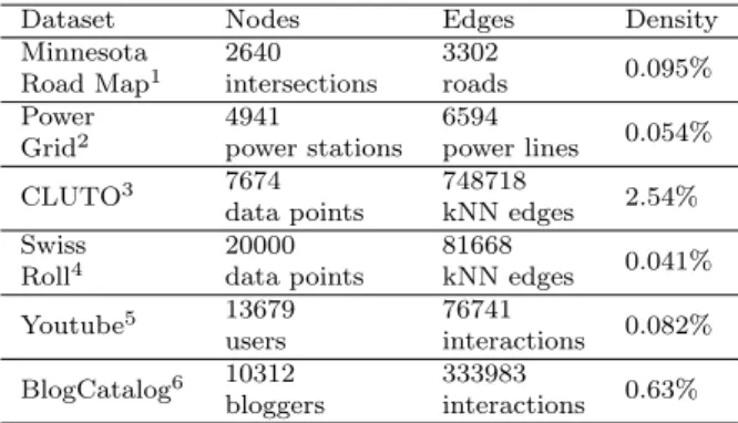
Table 2: Statistics of Datasets
Dataset Nodes Edges Density
Minnesota Road Map1 2640 intersections 3302 roads 0.095% Power Grid2 4941 power stations 6594 power lines 0.054% CLUTO3 7674 data points 748718 kNN edges 2.54% Swiss Roll4 20000 data points 81668 kNN edges 0.041% Youtube5 13679 users 76741 interactions 0.082% BlogCatalog6 10312 bloggers 333983 interactions 0.63%
second experiment, we compare the consistency of eigenpairs obtained from Incremental-IO and the batch method. For the third experiment, we use six popular graph datasets as listed in Table 2. The descriptions of these datasets are as follows.
1. Minnesota Road Map dataset is a graphical representation of roads in Minnesota, where nodes represent road intersections and edges represent roads.
2. Power Grid is a graph representing the topology of Western Power Grid of USA, where nodes represent power stations and edges represent power lines.
3. CLUTO is a synthetic dataset of two-dimensional data points for density-based clustering.
4. Swiss Roll is a synthetic dataset designed for manifold learning tasks. The data points lies in a two-dimensional manifold of a three-dimensional space. 5. Youtube is a graph representing social interactions of users on Youtube,
where nodes are users and edges are existence of interactions.
6. BlogCatalog is a social friendship graph among bloggers, where nodes rep-resent bloggers and edges reprep-resent their social interactions.
Among all six datasets, Minnesota Road Map and Power Grid are un-weighted graphs, and the others are un-weighted graphs. For CLUTO and Swiss Roll we usek-nearest neighbor (KNN) algorithm to generate similarity graphs, where the parameterk is the minimal value that makes the graph connected, and the similarity is measured by Gaussian kernel with unity bandwidth [57].
1 http://www.cs.purdue.edu/homes/dgleich/nmcomp/matlab/minnesota 2 http://www-personal.umich.edu/ mejn/netdata 3 http://glaros.dtc.umn.edu/gkhome/views/cluto 4 http://isomap.stanford.edu/datasets.html 5 http://socialcomputing.asu.edu/datasets/YouTube 6 http://socialcomputing.asu.edu/datasets/BlogCatalog
0 2 4 6 8 10 12 −50 0 50 100 150 200 250 300 350 400 450 number of eigenpairs K
computation time (seconds)
n=10000 batch method Lanczos−IO Incremental−IO (a) 0 2000 4000 6000 8000 10000 12000 100 101 102 103 number of nodes n
computation time in log scale (seconds)
K=10 batch method Lanczos−IO Incremental−IO
(b)
Fig. 1: Sequential eigenpair computation time on Erdos-Renyi random graphs with edge connection probability p = 0.1. The marker represents averaged computation time of 50 trials and the error bar represents standard deviation. (a) Computation time withn= 10000 and different number of eigenpairsK. It is observed that the computation time of Incremental-IO and Lanczos-IO grows linearly as K increases, whereas the computation time of the batch method grows superlinearly withK. (b) Computation time withK= 10 and different number of nodesn. It is observed that the difference in computation time between the batch method and the two incremental methods grow poly-nomially asnincreases, which suggests that in this experiment Incremental-IO and Lanczos-IO are more efficient than the batch computation method, espe-cially for large graphs.
6.1 Comparison of computation time on simulated graphs
To illustrate the advantage of Incremental-IO, we compare its computation time with the other two methods, the batch method and Lanczos-IO, for vary-ing order K and varying graph size n. The Erdos-Renyi random graphs that we build are used for this comparison. Fig. 1 (a) shows the computation time of Incremental-IO, Lanczos-IO, and the batch computation method for sequen-tially computing from K = 2 to K = 10 smallest eigenpairs. It is observed that the computation time of Incremental-IO and Lanczos-IO grows linearly as K increases, whereas the computation time of the batch method grows superlinearly withK.
Fig. 1 (b) shows the computation time of all three methods with respect to different graph sizen. It is observed that the difference in computation time between the batch method and the two incremental methods grow polyno-mially asn increases, which suggests that in this experiment Incremental-IO and Lanczos-IO are more efficient than the batch computation method, espe-cially for large graphs. It is worth noting that although Lanczos-IO has simi-lar performance in computation time as Incremental-IO, it requires additional memory allocation for storing all previously computed Lanczos vectors.
Minnesota RoadPower Grid CLUTO Swiss Roll Youtube BlogCatalog 0 100 101 102 103 tim e_b atc h tim e_i nc rem en tal (lo g sc ale )
Cluster Count = 5
Cluster Count = 10
Cluster Count = 15
Cluster Count = 20
Fig. 2: Computation time improvement of Incremental-IO relative to the batch method. Incremental-IO outperforms the batch method for all cases, and has improvement with respect toK.
6.2 Comparison of computation time on real-life datasets
Fig. 2 shows the time improvement of Incremental-IO relative to the batch method for the real-life datasets listed in Table 2, where the difference in computation time is displayed in log scale to accommodate large variance of time improvement across datasets that are of widely varying size. It is observed that the gain in computational time via Incremental-IO is more pronounced as cluster count K increases, which demonstrates the merit of the proposed incremental method.
On the other hand, although Lanczos-IO is also an incremental method, in addition to the well-known issue of requiring memory allocation for storing all Lanczos vectors, the experimental results show that it does not provide performance robustness as Incremental-IO does, as it can perform even worse than the batch method for some cases. Fig. 3 shows that Lanczos-IO actu-ally results in excessive computation time compared with the batch method for four out of the six datasets, whereas in Fig. 2 Incremental-IO is superior than the batch method for all these datasets, which demonstrates the robust-ness of Incremental-IO over Lanczos-IO. The reason of lacking robustrobust-ness for Lanczos-IO can be explained by the fact that the previously computed Lanc-zos vectors may not be effective in minimizing the Ritz approximation error of the desired eigenpairs. In contrast, Incremental-IO and the batch method adopt the implicitly-restarted Lanczos method, which restarts the Lanczos
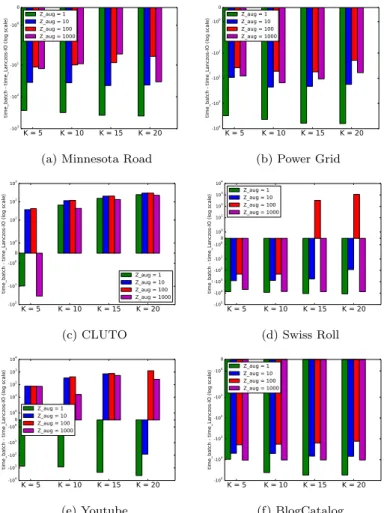
Minnesota RoadPower Grid CLUTO Swiss Roll Youtube BlogCatalog -104 -103 -102 -101 -1000 100 101 102 103 tim e_b atc h tim e_L an cz os-IO (lo g sc ale ) Cluster Count = 5 Cluster Count = 10 Cluster Count = 15 Cluster Count = 20
Fig. 3: Computation time improvement of Lanczos-IO relative to the batch method. Negative values mean that Lanczos-IO requires more computation time than the batch method. The results suggest that Lanczos-IO is not a robust incremental computation method, as it can perform even worse than the batch method for some cases.
algorithm when the generated Lanczos vectors fail to meet the Ritz approxi-mation criterion, and may eventually lead to faster convergence. Furthermore, Fig. 4 shows that Lanczos-IO is overly sensitive to the number of augmented Lanczos vectorsZaug, which is a parameter that cannot be optimizeda priori.
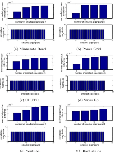
Theorem1 establishes that the proposed incremental method (Incremental-IO) exactly computes theK-th eigenpair using 1 to (K−1)-th eigenpairs, yet for the sake of experiments with real datasets, we have computed the normed eigenvalue difference (in terms of root mean squared error) and the corre-lations of the K smallest eigenvectors obtained from the batch method and Incremental-IO. As displayed in Fig. 5, theK smallest eigenpairs are identical as expected; to be more specific, using Matlab library, on the Minnesota road dataset forK= 20, the normed eigenvalue difference is 7×10⁻¹²and the asso-ciated eigenvectors are identical up to differences in sign. For all datasets listed in Table 2, the normed eigenvalue difference is negligible and the associated eigenvectors are identical up to the difference in sign, i.e., the eigenvector corre-lation in magnitude equals to 1 for every pair of corresponding eigenvectors of the two methods, which verifies the correctness of Incremental-IO. Moreover, due to the eigenpair consistency between the batch method and Incremental-IO as demonstrated in Fig. 5, they yield the same clustering results in the considered datasets.
K = 5 K = 10 K = 15 K = 20 -103 -102 -101 -100 0 tim e_b atc h tim e_L an cz os-IO (lo g sc ale ) Z_aug = 1Z_aug = 10 Z_aug = 100 Z_aug = 1000
(a) Minnesota Road
K = 5 K = 10 K = 15 K = 20 -104 -103 -102 -101 -100 0 tim e_b atc h tim e_L an cz os-IO (lo g sc ale ) Z_aug = 1Z_aug = 10 Z_aug = 100 Z_aug = 1000 (b) Power Grid K = 5 K = 10 K = 15 K = 20 -102 -101 -100 0 100 101 102 103 tim e_b atc h tim e_L an cz os-IO (lo g sc ale ) Z_aug = 1 Z_aug = 10 Z_aug = 100 Z_aug = 1000 (c) CLUTO K = 5 K = 10 K = 15 K = 20 -105 -104 -103 -102 -101 -1000 100 101 102 103 104 tim e_b atc h tim e_L an cz os-IO (lo g sc ale ) Z_aug = 1Z_aug = 10 Z_aug = 100 Z_aug = 1000 (d) Swiss Roll K = 5 K = 10 K = 15 K = 20 -104 -103 -102 -101 -1000 100 101 102 103 104 tim e_b atc h tim e_L an cz os-IO (lo g sc ale ) Z_aug = 1 Z_aug = 10 Z_aug = 100 Z_aug = 1000 (e) Youtube K = 5 K = 10 K = 15 K = 20 -105 -104 -103 -102 -101 -100 0 tim e_b atc h tim e_L an cz os-IO (lo g sc ale ) Z_aug = 1Z_aug = 10 Z_aug = 100 Z_aug = 1000 (f) BlogCatalog
Fig. 4: The effect of number of augmented Lanczos vectors Zaug of
Lanczos-IO in Algorithm3 on computation time improvement relative to the batch method. Negative values mean that the computation time of Lanczos-IO is larger than that of the batch method. The results show that Lanczos-IO is not a robust incremental eigenpair computation method. Intuitively, small Zaug
may incur many iterations in the second step of Algorithm 3, whereas large Zaug may pose computation burden in the first step of Algorithm 3, and
therefore both cases lead to the increase in computation time.
6.3 Clustering metrics for user-guided spectral clustering
In real-life, an analyst can use Incremental-IO for clustering along with a mech-anism for selecting the best choice ofKstarting fromK= 2. To demonstrate this, in the experiment we use five clustering metrics that can be used for online decision making regarding the value ofK. These metrics are commonly
5 10 15 20 0 2 4 6 8x 10 −12
number of smallest eigenpairs K
normed eigenvalue difference 0 5 10 15 20 25 0 0.5 1 1.5 smallest eigenpairs correlation magnitude
(a) Minnesota Road
5 10 15 20 0 2 4 6 8x 10 −11
number of smallest eigenpairs K
normed eigenvalue difference 0 5 10 15 20 25 0 0.5 1 1.5 smallest eigenpairs correlation magnitude (b) Power Grid 5 10 15 20 0 1 2 3 4x 10 −11
number of smallest eigenpairs K
normed eigenvalue difference 0 5 10 15 20 25 0 0.5 1 1.5 smallest eigenpairs correlation magnitude (c) CLUTO 5 10 15 20 0 2 4 6 8x 10 −11
number of smallest eigenpairs K
normed eigenvalue difference 0 5 10 15 20 25 0 0.5 1 1.5 smallest eigenpairs correlation magnitude (d) Swiss Roll 5 10 15 20 0 1 2 3 4x 10 −10
number of smallest eigenpairs K
normed eigenvalue difference 0 5 10 15 20 25 0 0.5 1 1.5 smallest eigenpairs correlation magnitude (e) Youtube 5 10 15 20 0 0.5 1x 10 −11
number of smallest eigenpairs K
normed eigenvalue difference 0 5 10 15 20 25 0 0.5 1 1.5 smallest eigenpairs correlation magnitude (f) BlogCatalog
Fig. 5: Consistency of smallest eigenpairs computed by the batch computa-tion method and Incremental-IO for datasets listed in Table 2. The normed eigenvalue difference is the square root of sum of squared differences between eigenvalues. The correlation magnitude is the absolute value of inner product of eigenvectors, where 1 means perfect alignment.
used in clustering unweighted and weighted graphs and they are summarized as follows.
1. Modularity:modularity is defined as Mod = K X i=1 W(C i,Ci) W(V,V) − W(C i,V) W(V,V) 2 , (11)
where V is the set of all nodes in the graph, Ci is the i-th cluster, W(Ci,Ci)
i-th cluster, W(Ci,V) = W(Ci,Ci) +W(Ci,Ci), and W(V,V) = Pn
j=1sj =s
denotes the total nodal strength.
2. Scaled normalized cut (SNC):NC is defined as [57] NC = K X i=1 W(Ci,Ci) W(Ci,V) . (12)
SNC is NC divided by the number of clusters, i.e., NC/K.
3. Scaled median (or maximum) cluster size:Scaled medium (maximum) cluster size is the medium (maximum) cluster size of K clusters divided by the total number of nodesnof a graph.
4. Scaled spectrum energy: scaled spectrum energy is the sum of theK smallest eigenvalues of the graph Laplacian matrix L divided by the sum of all eigenvalues ofL, which can be computed by
scaled spectrum energy =
PK
i=1λi(L)
Pn
j=1Ljj
, (13)
where λi(L) is the i-th smallest eigenvalue ofL and Pn
j=1Ljj =
Pn
i=1λi(L)
is the sum of diagonal elements ofL.
These metrics provide alternatives for gauging the quality of the clustering method. For example, Mod and NC reflect the trade-off between intracluster similarity and intercluster separation. Therefore, the larger the value of Mod, the better the clustering quality, and the smaller the value of NC, the better the clustering quality. Scaled spectrum energy is a typical measure of cluster quality for spectral clustering [34, 40, 58], and smaller spectrum energy means better separability of clusters. For Mod and scaled NC, a user might look for a cluster countK such that the increment in the clustering metric is not significant, i.e., the clustering metric is saturated beyond such aK. For scaled median and maximum cluster size, a user might require the cluster countK to be such that the clustering metric is below a desired value. For scaled spectrum energy, a user might look for a noticeable increase in the clustering metric between consecutive values ofK.
6.4 Demonstration
Here we use Minnesota Road data to demonstrate how users can utilize the clustering metrics in Sec. 6.3 to determine the number of clusters. For exam-ple, the five metrics evaluated for Minnesota Road clustering with respect to different cluster counts K are displayed in Fig. 6 (a). Starting from K = 2 clusters, these metrics are updated by the incremental user-guided spectral clustering algorithm (Algorithm2) asK increases. If the user imposes that the maximum cluster size should be less than 30% of the total number of nodes, then the algorithm returns clustering results with a number of clusters ofK= 6 or greater. Inspecting the modularity one sees it saturates atK= 7, and the user also observes a noticeable increase in scaled spectrum energy
2 3 4 5 6 7 8 9 10 0 0.51 modularity 2 3 4 5 6 7 8 9 10 0 0.02 0.04 NC/K 2 3 4 5 6 7 8 9 10 0 0.5
median cluster size/n
2 3 4 5 6 7 8 9 10
0 0.51
maximum cluster size/n
2 3 4 5 6 7 8 9 10
0 0.51
x 10−5 scaled spectrum energy
K
(a) Minnesota Road
2 4 6 8 10 12 14 16 18 20 0 0.51 modularity 2 4 6 8 10 12 14 16 18 20 0 0.02 0.04 NC/K 2 4 6 8 10 12 14 16 18 20 0
0.5 median cluster size/n
2 4 6 8 10 12 14 16 18 20
0 0.5
1 maximum cluster size/n
2 4 6 8 10 12 14 16 18 20 0 0.5 1x 10 −5 spectrum energy K (b) Power Grid 2 4 6 8 10 12 14 16 18 20 0 0.5 1 modularity 2 4 6 8 10 12 14 16 18 20 0 0.02 0.04 NC/K 2 4 6 8 10 12 14 16 18 20 0 0.5
median cluster size/n
2 4 6 8 10 12 14 16 18 20
0 0.51
maximum cluster size/n
2 4 6 8 10 12 14 16 18 20 0 1 2x 10 −6 spectrum energy K (c) Swiss Roll 2 4 6 8 10 12 14 16 18 20 0 0.5 1 modularity 2 4 6 8 10 12 14 16 18 20 0 0.05 0.1 NC/K 2 4 6 8 10 12 14 16 18 20 0 0.5
median cluster size/n
2 4 6 8 10 12 14 16 18 20
0 0.51
maximum cluster size/n
2 4 6 8 10 12 14 16 18 20 0 1 2x 10 −4 spectrum energy K (d) CLUTO 2 4 6 8 10 12 14 16 18 20 0 0.5 modularity 2 4 6 8 10 12 14 16 18 20 0 0.1 0.2 NC/K 2 4 6 8 10 12 14 16 18 20 0
0.5 median cluster size/n
2 4 6 8 10 12 14 16 18 20
0.6 0.81
maximum cluster size/n
2 4 6 8 10 12 14 16 18 20 0 5x 10 −5 spectrum energy K (e) Youtube 2 4 6 8 10 12 14 16 18 20 −0.2 0 0.2 modularity 2 4 6 8 10 12 14 16 18 20 0.6 0.81 NC/K 2 4 6 8 10 12 14 16 18 20 0
0.5 median cluster size/n
2 4 6 8 10 12 14 16 18 20
0 0.5
1 maximum cluster size/n
2 4 6 8 10 12 14 16 18 20 0 0.51 x 10⁻⁴ spectrum energy K (f) BlogCatalog
Fig. 6: Five clustering metrics computed incrementally viaAlgorithm 2 for different datasets listed in Table 2. The metrics are modularity, scaled nor-malized cut (NC/K), scaled median and maximum cluster size, and scaled spectrum energy. These clustering metrics are used to help users determine the number of clusters.
whenK= 7. Therefore, the algorithm can be used to incrementally generate four clustering results for K= 7,8,9, and 10. The selected clustering results in Fig. 7 are shown to be consistent with geographic separations of different granularity.
We also apply the proposed incremental user-guided spectral clustering algorithm (Algorithm 2) to Power Grid, CLUTO, Swiss Roll, Youtube, and BlogCatalog. In Fig. 6, we show how the values of clustering metrics change with K for each dataset. The incremental method enables us to efficiently generate all clustering results withK= 2,3,4. . .and so on. It can be observed
(a)K= 7 (b)K= 8
(c)K= 9 (d)K= 10
Fig. 7: Visualization of user-guided spectral clustering on Minnesota Road with respect to selected cluster countK. Colors represent different clusters.
from Fig. 6 that for each dataset the clustering metric that exhibits the highest variation inKcan be different. This suggests that selecting the correct number of clusters is a difficult task and a user might need to use different clustering metrics for a range of K values, and Incremental-IO is an effective tool to support such an endeavor.
7 Conclusion
In this paper we present Incremental-IO, an efficient incremental eigenpair computation method for graph Laplacian matrices which works by transform-ing a batch eigenvalue decomposition problem into a sequential leadtransform-ing eigen-pair computation problem. The method is elegant, robust and easy to imple-ment using a scientific programming language, such as Matlab. We provide analytical proof of its correctness. We also demonstrate that it achieves signif-icant reduction in computation time when compared with the batch compu-tation method. Particularly, it is observed that the difference in compucompu-tation time of these two methods grows polynomially as the graph size increases.
To demonstrate the effectiveness of Incremental-IO, we also show experi-mental evidences that obtaining such an increexperi-mental method by adapting the existing leading eigenpair solvers (such as, the Lanczos algorithm) is non-trivial and such efforts generally do not lead to a robust solution.
Finally, we demonstrate that the proposed incremental eigenpair compu-tation method (Incremental-IO) is an effective tool for a user-guided spectral clustering task, which effectively updates clustering results and metrics for each increment of the cluster count.
Acknowledgments
This research is sponsored by Mohammad Al Hasan’s NSF CAREER Award (IIS-1149851). The contents are solely the responsibility of the authors and do not necessarily represent the official view of NSF.
References
1. S. Basu, A. Banerjee, and R. J. Mooney. Active semi-supervision for pairwise con-strained clustering. InSDM, volume 4, pages 333–344, 2004.
2. M. Belkin and P. Niyogi. Laplacian eigenmaps for dimensionality reduction and data representation. Neural computation, 15(6):1373–1396, 2003.
3. V. D. Blondel, J.-L. Guillaume, R. Lambiotte, and E. Lefebvre. Fast unfolding of com-munities in large networks. Journal of Statistical Mechanics: Theory and Experiment, (10), 2008.
4. D. Calvetti, L. Reichel, and D. C. Sorensen. An implicitly restarted lanczos method for large symmetric eigenvalue problems.Electronic Transactions on Numerical Analysis, 2(1):21, 1994.
5. J. Chen, L. Wu, K. Audhkhasi, B. Kingsbury, and B. Ramabhadrari. Efficient one-vs-one kernel ridge regression for speech recognition. InIEEE International Conference on Acoustics, Speech and Signal Processing (ICASSP), pages 2454–2458, 2016. 6. P.-Y. Chen and A. Hero. Deep community detection. 63(21):5706–5719, Nov. 2015. 7. P.-Y. Chen and A. Hero. Phase transitions in spectral community detection.
63(16):4339–4347, Aug 2015.
8. P.-Y. Chen and A. O. Hero. Node removal vulnerability of the largest component of a network. InGlobalSIP, pages 587–590, 2013.
9. P.-Y. Chen and A. O. Hero. Assessing and safeguarding network resilience to nodal attacks. 52(11):138–143, Nov. 2014.
10. P.-Y. Chen and A. O. Hero. Phase transitions and a model order selection criterion for spectral graph clustering.arXiv preprint arXiv:1604.03159, 2016.
11. P.-Y. Chen and A. O. Hero. Multilayer spectral graph clustering via convex layer aggregation: Theory and algorithms. IEEE Transactions on Signal and Information Processing over Networks, 3(3):553–567, Sept 2017.
12. P.-Y. Chen and S. Liu. Bias-variance tradeoff of graph laplacian regularizer. IEEE Signal Processing Letters, 24(8):1118–1122, Aug 2017.
13. P.-Y. Chen and L. Wu. Revisiting spectral graph clustering with generative community models.arXiv preprint arXiv:1709.04594, 2017.
14. P.-Y. Chen, B. Zhang, M. A. Hasan, and A. O. Hero. Incremental method for spectral clustering of increasing orders. InKDD Workshop on Mining and Learning with Graphs, 2016.
15. S. Choudhury, K. Agarwal, S. Purohit, B. Zhang, M. Pirrung, W. Smith, and M. Thomas. NOUS: construction and querying of dynamic knowledge graphs. In Pro-ceedings of 33rd IEEE International Conference on Data Engineering, pages 1563–1565, 2017.
16. F. R. K. Chung. Spectral Graph Theory. American Mathematical Society, 1997. 17. C. Dhanjal, R. Gaudel, and S. Cl´emen¸con. Efficient eigen-updating for spectral graph
18. M. Dundar, Q. Kou, B. Zhang, Y. He, and B. Rajwa. Simplicity of kmeans versus deepness of deep learning: A case of unsupervised feature learning with limited data. InProceedings of 14th IEEE International Conference on Machine Learning and Ap-plications, pages 883–888, 2015.
19. M. A. Hasan, V. Chaoji, S. Salem, and M. Zaki. Link prediction using supervised learning. InIn Proc. of SDM 06 workshop on Link Analysis, Counterterrorism and Security, 2006.
20. M. A. Hasan and M. J. Zaki. A Survey of Link Prediction in Social Networks, pages 243–275. Springer US, 2011.
21. R. A. Horn and C. R. Johnson. Matrix Analysis. Cambridge University Press, 1990. 22. P. Jia, J. Yin, X. Huang, and D. Hu. Incremental laplacian eigenmaps by preserving
adjacent information between data points. Pattern Recognition Letters, 30(16):1457– 1463, 2009.
23. F. Krzakala, C. Moore, E. Mossel, J. Neeman, A. Sly, L. Zdeborova, and P. Zhang. Spectral redemption in clustering sparse networks.Proc. National Academy of Sciences, 110:20935–20940, 2013.
24. J. Kuczynski and H. Wozniakowski. Estimating the largest eigenvalue by the power and lanczos algorithms with a random start. SIAM journal on matrix analysis and applications, 13(4):1094–1122, 1992.
25. C. Lanczos. An iteration method for the solution of the eigenvalue problem of lin-ear differential and integral operators. Journal of Research of the National Bureau of Standards, 45(4), 1950.
26. R. M. Larsen. Computing the svd for large and sparse matrices. SCCM, Stanford University, June, 16, 2000.
27. R. B. Lehoucq, D. C. Sorensen, and C. Yang.ARPACK users’ guide: solution of large-scale eigenvalue problems with implicitly restarted Arnoldi methods, volume 6. Siam, 1998.
28. S. Liu, H. Chen, S. Ronquist, L. Seaman, N. Ceglia, W. Meixner, L. A. Muir, P.-Y. Chen, G. Higgins, P. Baldi, et al. Genome architecture leads a bifurcation in cell identity.bioRxiv, page 151555, 2017.
29. S. Liu, P.-Y. Chen, and A. O. Hero. Accelerated distributed dual averaging over evolving networks of growing connectivity. arXiv preprint arXiv:1704.05193, 2017.
30. W. Liu, P.-Y. Chen, S. Yeung, T. Suzumura, and L. Chen. Principled multilayer network embedding.CoRR, abs/1709.03551, 2017.
31. W. J. Lu, C. Xu, Z. Pei, A. S. Mayhoub, M. Cushman, and D. A. Flockhart. The tamox-ifen metabolite norendoxtamox-ifen is a potent and selective inhibitor of aromatase (CYP19) and a potential lead compound for novel therapeutic agents. Breast Cancer Research and Treatment, 133(1):99–109, 2012.
32. U. Luxburg. A tutorial on spectral clustering.Statistics and Computing, 17(4):395–416, Dec. 2007.
33. R. Merris. Laplacian matrices of graphs: a survey.Linear Algebra and its Applications, 197-198:143–176, 1994.
34. A. Y. Ng, M. I. Jordan, and Y. Weiss. On spectral clustering: Analysis and an algorithm. InNIPS, pages 849–856, 2002.
35. H. Ning, W. Xu, Y. Chi, Y. Gong, and T. S. Huang. Incremental spectral clustering with application to monitoring of evolving blog communities. InSDM, pages 261–272, 2007.
36. H. Ning, W. Xu, Y. Chi, Y. Gong, and T. S. Huang. Incremental spectral clustering by efficiently updating the eigen-system.Pattern Recognition, 43(1):113–127, 2010. 37. R. Olfati-Saber, J. Fax, and R. Murray. Consensus and cooperation in networked
multi-agent systems. 95(1):215–233, 2007.
38. B. N. Parlett. The symmetric eigenvalue problem, volume 7. SIAM, 1980.
39. Z. Pei, Y. Xiao, J. Meng, A. Hudmon, and T. R. Cummins. Cardiac sodium channel palmitoylation regulates channel availability and myocyte excitability with implications for arrhythmia generation. Nature Communications, 7, 2016.
40. M. Polito and P. Perona. Grouping and dimensionality reduction by locally linear embedding. InNIPS, 2001.
41. L. K. M. Poon, A. H. Liu, T. Liu, and N. L. Zhang. A model-based approach to rounding in spectral clustering. InUAI, pages 68–694, 2012.
42. A. Pothen, H. D. Simon, and K.-P. Liou. Partitioning sparse matrices with eigenvectors of graphs.SIAM journal on matrix analysis and applications, 11(3):430–452, 1990. 43. F. Radicchi and A. Arenas. Abrupt transition in the structural formation of
intercon-nected networks.Nature Physics, 9(11):717–720, Nov. 2013.
44. G. Ranjan, Z.-L. Zhang, and D. Boley. Incremental computation of pseudo-inverse of laplacian. InCombinatorial Optimization and Applications, pages 729–749. Springer, 2014.
45. A. Saade, F. Krzakala, M. Lelarge, and L. Zdeborova. Spectral detection in the censored block model.arXiv:1502.00163, 2015.
46. T. K. Saha, B. Zhang, and M. Al Hasan. Name disambiguation from link data in a collaboration graph using temporal and topological features. Social Network Analysis Mining, 5(1):11:1–11:14, 2015.
47. J. Shi and J. Malik. Normalized cuts and image segmentation. 22(8):888–905, 2000. 48. D. Shuman, S. Narang, P. Frossard, A. Ortega, and P. Vandergheynst. The
emerg-ing field of signal processemerg-ing on graphs: Extendemerg-ing high-dimensional data analysis to networks and other irregular domains. 30(3):83–98, 2013.
49. S. M. Van Dongen. Graph clustering by flow simulation. PhD thesis, University of Utrecht, 2000.
50. S. White and P. Smyth. A spectral clustering approach to finding communities in graph. InSDM, volume 5, pages 76–84, 2005.
51. K. Wu and H. Simon. Thick-restart lanczos method for large symmetric eigenvalue problems.SIAM Journal on Matrix Analysis and Applications, 22(2):602–616, 2000. 52. L. Wu, J. Laeuchli, V. Kalantzis, A. Stathopoulos, and E. Gallopoulos. Estimating the
trace of the matrix inverse by interpolating from the diagonal of an approximate inverse.
Journal of Computational Physics, 326:828–844, 2016.
53. L. Wu, M. Q.-H. Meng, Z. Dong, and H. Liang. An empirical study of dv-hop localiza-tion algorithm in random sensor networks. InInternational Conference on Intelligent Computation Technology and Automation, volume 4, pages 41–44, 2009.
54. L. Wu, E. Romero, and A. Stathopoulos. Primme svds: A high-performance precon-ditioned svd solver for accurate large-scale computations. SIAM Journal on Scientific Computing, 39(5):S248–S271, 2017.
55. L. Wu and A. Stathopoulos. A preconditioned hybrid svd method for accurately com-puting singular triplets of large matrices. SIAM Journal on Scientific Computing, 37(5):S365–S388, 2015.
56. L. Wu, I. E. Yen, J. Chen, and R. Yan. Revisiting random binning features: Fast convergence and strong parallelizability. InACM SIGKDD International Conference on Knowledge Discovery and Data Mining, pages 1265–1274, 2016.
57. M. J. Zaki and W. M. Jr. Data Mining and Analysis: Fundamental Concepts and Algorithms. Cambridge University Press, 2014.
58. L. Zelnik-Manor and P. Perona. Self-tuning spectral clustering. InNIPS, pages 1601– 1608, 2004.
59. B. Zhang, S. Choudhury, M. A. Hasan, X. Ning, K. Agarwal, and S. P. andy Paola Pesantez Cabrera. Trust from the past: Bayesian personalized ranking based link pre-diction in knowledge graphs. InSDM MNG Workshop, 2016.
60. B. Zhang, M. Dundar, and M. A. Hasan. Bayesian non-exhaustive classification a case study: Online name disambiguation using temporal record streams. InProceedings of the 25th ACM International on Conference on Information and Knowledge Management, pages 1341–1350. ACM, 2016.
61. B. Zhang, M. Dundar, and M. A. Hasan. Bayesian non-exhaustive classification for active online name disambiguation.arXiv preprint arXiv:1702.02287, 2017.
62. B. Zhang and M. A. Hasan. Name disambiguation in anonymized graphs using net-work embedding. InProceedings of the 26th ACM International on Conference on Information and Knowledge Management, 2017.
63. B. Zhang, N. Mohammed, V. S. Dave, and M. A. Hasan. Feature selection for classifi-cation under anonymity constraint.Transactions on Data Privacy, 10(1):1–25, 2017. 64. B. Zhang, T. K. Saha, and M. A. Hasan. Name disambiguation from link data in a
collaboration graph. InASONAM, pages 81–84, 2014.
View publication stats View publication stats