Traffic Volume Modelling in Parallel Computing Environment

(1)

University of West Bohemia

Faculty of applied sciences

Department of Geomatics

Traffic Volume Modeling in Parallel

Computing Environment

Master Thesis

Frantiˇ

sek Kolovsk´

y

(2)

Declaration

I declare that this thesis is my original work of authorship that I have created myself. All resources, sources and literature, which I used in my thesis, is cited indicating the full link to the appropriate source.

In Pilsen ... ... Frantiˇsek Kolovsk´y

Acknowledgment

I thank to my supervisor Jan Jeˇzek for comments and methodical guidance. Ac-cess to computing and storage facilities owned by parties and projects contribut-ing to the National Grid Infrastructure MetaCentrum, provided under the pro-gramme ”Projects of Large Infrastructure for Research, Development, and Inno-vations” (LM2010005), is greatly appreciated.

(3)

Abstract

Nowadays, a lot of transport-related data for a traffic modeling are available, but present software tools that can process such data volume and compute large models are still lacking. The aim of this thesis is to analyse, design and test an imple-mentation of the transport models in the scalable parallel computing environment. More particularly, the work is primarily focused on the Origin-Destination matrix estimation and the traffic assignment, which are the essential parts for traffic volume modeling. Parallel algorithms that are suitable for such a problem are described, evaluated and implemented into the Map-Reduce computing model (Apache Spark is used for such a purpose). Implemented methods are tested on various-sized datasets and the test results are demonstrated . Experiments have shown, that the proposed solution is capable of processing a large-scale model (e.g. a model of whole Europe consisting of millions of edges) within a time frame of tens of hours.

Key words

Map-Reduce, Origin-Destination matrix estimation, traffic assignment, distributed environment, Apache Spark, traffic volume, parallel computing

(4)

Abstrakt

V posledn´ıch letech je k dispozici stále v´ıce dat vhodných jako podklad pro výpoˇcet dopravn´ıch intenzit, ale softwarové nástroje pro tvorbu velkých model˚u z tˇechto dat nejsou dostupné. C´ılem této práce je analyzovat, navrhnout a otestovat imple-mentaci transportn´ıch model˚u ve ˇskálovatelném paraleln´ım výpoˇcetn´ım prostˇred´ı. Práce se pˇredevˇs´ım zamˇeˇruje na odhad matice pˇrepravn´ıch vztah˚u a na pˇridˇelován´ı zátˇeˇze na s´ıˇt. Vhodné paraleln´ı algoritmy jsou popsány, vyhodnoceny a imple-mentovány ve výpoˇcetn´ım prostˇred´ı typu MapReduce (pro tento úˇcel je pouˇz´ıván Apache Spark). Implementované metody jsou testovány na datech o r˚uzné velikosti. Výsledky tˇechto test˚u ukazuj´ı, ˇze pomoc´ı vyvinutého frameworku lze vytvoˇrit velké modely (napˇr´ıklad model celé Evropy, který obsahuje milióny hran) v ˇrádu des´ıtek hodin.

Kl´ıˇ

cov´

a slova

Map-Reduce, odhad matice pˇrepravn´ıch vztah˚u, pˇridˇelován´ı zátˇeˇze na s´ıˇt, distribuo-vané výpoˇcetn´ı prostˇred´ı, Apache Spark, intenzity dopravy, paraleln´ı výpoˇcty

(5)

Introduction

In recent years, the traffic volume in road network increases. This puts higher demands on the traffic management through intelligent systems. One of the tools for the traffic management is a traffic modeling. A state-of-the-art traffic modeling approach is based on a 4-step transport model, that consists of four consecutive independent steps, where each step model one aspect of the transport.

Nowadays these transport models are mostly created by using proprietary soft-ware tools, that works in single-computer desktop environment. This way of creating the transport models is limited by the computational speed and memory size. As the size of the model and computational complexity increases, there is a rise of the demand for a scalable solution that will utilize the benefits of cloud computing. Such a solution might open many new possibilities to model large-scale networks.

This thesis aims to solve this problem by converting all the calculations into the distributed parallel computing environment. This work is especially focused on Origin-Destination matrix estimation and the traffic assignment.

The parallel algorithms for creating these models are going to be introduced in the upcoming text. The first chapter is focused on definition of the basic therms including 4-step transport model. The second chapter contains the problem formula-tion and introduces the methods of solving these problems. The detailed descripformula-tion of the implemented methods is in third chapter. The fourth chapter is focused on a implementation of chosen methods by using Apache Spark. The last part of this thesis contains the performance tests.

(8)

Chapter 1 Theoretic background

This chapter introduces the basic terminology and model data, that is used in the area of transport modeling. It focuses its relation to the programing model that is essential for upcoming chapters.

Furthermore, the memory and time complexity of the problem is described, such aspects represent a limiting factor for existing solutions.

Algorithms used in the area of transport modeling are further elaborated at the end of this chapter.

1.1 Basic terms definition

1.1.1 Graph

A graph is defined as a pair of sets

G=< V, A > (1.1)

where V is a set of vertices (nodes) andA is a set of edges (links)

A={{u, v}|u, v ∈V, u6=v} (1.2)

Oriented graph is a directed graph. Edge {u, v} is directed from u to v (can be crossed only fromu to v).

Vertex degree is number of edges that start or end in a vertex. If edge starts and ends in the same vertex, the degree is increased by two.

(9)

A path is a sequence of the edges (vertices).

1.1.2 Transport modeling

A zone is a place, which at least one path starts or ends. The zone can be region, district of the city or block of buildings. The size of the zones depends on details of the model.

The number of the trips that begin and end in the zone is a main property of the zone. Real world example of a trip can be a path from home to work by car.

1.2 Macro Traffic Volume Model

The traffic model tries to model the transport in the area of interest. The model is created by considering detailed knowledge of the area and theoretical assumptions about human behavior.

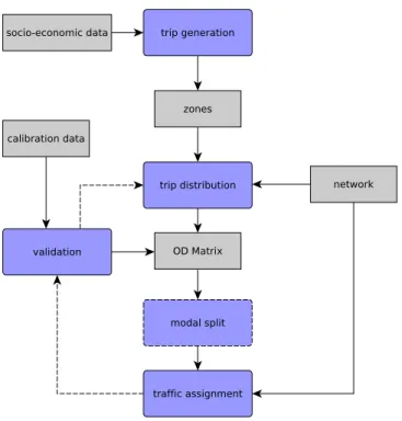
One of the most commonly used model is classic 4-step transport models, which has been used for more than 50 years. Even though some details have changed recently, the basic principles remain unchanged. The model consist of 4 consequence steps (sub-models). These steps are:

1) trip generation, which determines the number of the trips incoming/outcoming from/to the zones,

2) trip distribution, which determines the number of the trips between the zones, 3) modal split, which splits the trips between different modes of transport, 4) traffic assignment, which allocates the trips between the zones to the road

network thereby computes the traffic volume on every link.

Figure 1.1 depicts activity diagram of the transport modeling. Detailed descrip-tion is elaborated in upcoming secdescrip-tions.

(10)

Figure 1.1: Classic transport 4-step transport model

1.2.1 Trip generation

The main goal of this step is a determination of the number of the trips that begin and end in the zones. During the trip modeling, the focus is given to a personal trips. The number of personal trips is affected by many factors, that are very important in practical studies. The main factors are:

• income level, car ownership (number of cars), household size and structures (ages, gender, size),

• value of land, residential density (number of houses per area), accessibility (hard to determine it),

• roofed space for industrial, commercial and other services,

• number of employees, number of sales, total area of firm.

The first two groups of factors affect the personal trip production. The zone attrac-tion (income trips) is influenced by the last two groups [dDOW11].

For local model it is usually a simple task to obtain these detailed data, but for the large area of interest it might became hard (e.g Europe model).

(11)

1.2.2 Trip distribution

Trip distribution is the most important step. The aim of this step is to estimate the Origin-Destination Matrix (ODM). The ODM contains the number of the trips between all zones. One cell of the ODM is called OD pair. There are many different methods for estimating the ODM. This problem is further discussed in Section 2.2, 3.2 and 3.3.

The basic idea is that the number of the trips indirectly depends on a distance between two zones (travel time, generalized cost). More people are travelling shorter distance. As a consequence the cost matrix must be computed at first. Dijkstra’s algorithm can be used for such a purpose.

The input for this step is the road network (graph) and a set of the zones.

1.2.3 Modal split

Modal split is a process that splits the trips between more modes of transport (e.g bus, train, personal car, bike). The ODM is split into several matrices according to the type of transport (e.g public and private transport). If only the private transport is considered (or any other one type) in the previous steps, modal split can be skipped.

1.2.4 Traffic assignment

The last step of transport model determines a traffic volume on every link in the road network. The idea is that the drivers use an optimal path. The traffic volume on every link in the path is increased by the number of all trips between the source and the destination zone. There are two basic method of the traffic assignment [dDOW11]:

• no congestion effects (all-or-nothing),

(12)

Wardrop’s or Equilibrium assignment reflects the path choice by the actual traf-fic volume (congestion effect). Equilibrium state is searched in this case [War52], therefore the algorithms for this problem are iterative.

1.3 Time and memory complexity of the problem

Time and memory complexity are the main properties of the algorithm, so it is necessary be discussed in details. As stated above, the main problem of the macro traffic modeling is the process of searching the shortest paths. One of the most relevant algorithm for the shortest path search is the Dijkstra’s algorithm. The time complexity of Dijkstra (when a binary heap is used) is [Dij59]:

O(|A|+|V|log2|V|) (1.3)

whereA is set of edges,V is set of vertex (nodes). Fibonacci heap is more effective but its implementation is more complicated and most graph libraries use the binary heap [FT87].

The task of the traffic model is to find the shortest path for all zone pairs. It is

|Z|2_{− |}_Z_| _{paths. One Dijkstra’s search find} _|_Z_{| −}_{1 paths (shortest path tree). So}

the final complexity is:

O(|Z|(|A|+|V|log2|V|)) (1.4)

where Z is a set of the zones.

The number of the trips must be stored for every zone pair. This is |Z|2 _{− |}_Z_|

values. This implies, that memory demand increases quadratically with number of the zones. However, it is not necessary to consider all OD pairs in the large models, because the influence of two villages, which are very distant, is insignificant.

1.4 Existing software tools limitations

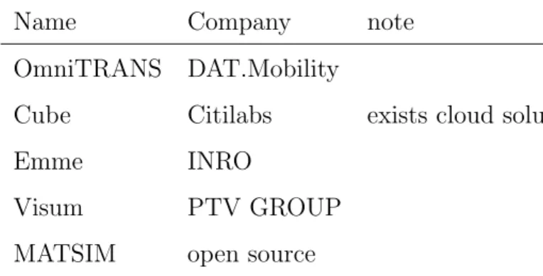
The most popular traffic modeling software for macro scale are OmniTRANS, Cube, Visum, Emme, MATSIM. All these solutions are based on the desktop environment (Cube has cloud version). In this thesis, the term ”desktop” means a personal computer with 8GB RAM and with one processor.

(13)

Name Company note OmniTRANS DAT.Mobility

Cube Citilabs exists cloud solution

Emme INRO

Visum PTV GROUP

MATSIM open source

Table 1.1: Tradition modeling software

The main motivation for this thesis was a discussion with transport modeling experts from a few reputable companies. The size of the model is often mentioned as one of the main problem, that limits the efficient use of assembled models and impossibility to create the large models. The model is composed from the road network (graph), zones and count profiles (reference values of traffic volume). Ac-cording to the findings from the previous section, the main limitation is the size of the network and the number of zones.

For example, the shortest path searching for Czech Republic model, where the set of zones has 7000 items (every village and city district) and the road network has 3 mil. edges (including all relevant roads), takes more than 4 hours (one Dijkstra’s search takes 2 s) and more than 196 MB for storing OD Matrix (one cell in ODM takes 4 bytes (double)). This model can be easily computed by a commodity desktop computer. However, more accurate model with 22 000 zones (real model created by reputable company) can not be calculated by conventional modeling software, because exceeds the memory limits and processor performance.

One of the relevant approach to deal with this limitations is the usage of the distributed computing environment for large models.

1.5 Map-Reduce parallel computing model

Map-reduce is a high level programming model for processing a large set of data. The model was published in 2008 by [DG08]. There are many cluster-based computing systems that implements such the model (e.g Apache Hadoop, Apache Spark, Google

(14)

File System (GFS)). Nowadays, the Map-reduce might be considered as one of the most popular programming model for processing big data.

Map-reduce is based on two basic operations: Map and Reduce. The map and the reduce functions are running with a set of data in a parallel across the whole cluster.

The map operation is a transformation function, that transforms every item in the set of data. Usually (not always) the size of an input dataset is the same as the size of an output dataset. For example, the transportation function splits every line (input item) from a text file to words and counts them. So the output will contain integers (number of words in line).

Reduce operation combines the items in the dataset and reduces their number according to a combiner function. For example, when the combiner function ”plus” (a+b) will be applied to the output dataset from the previous paragraph, the result will be the number of the word in the whole text.

In general, the input of the map function is a pair (key, value) and the output is a list of transformed (key, value) (cardinality is 1 - N). The input of the reduce function is a key and a list of values (usually 2 item) and the output is the key and one value computed from the list of the input values (cardinality is N - 1).

operation input output

map (k1, v1) → list(k2, v2) reduce (k2, list(v2)) → (k2, v2)

1.6 Algorithm for optimization

In this Section well-known algorithms focused on the optimization are going to be described.

1.6.1 Frank-Wolfe

Frank-Wolfe algorithm (FWA) is the first-order minimization algorithm for a con-strained convex problem. FWA solves minimization problem:

min

(15)

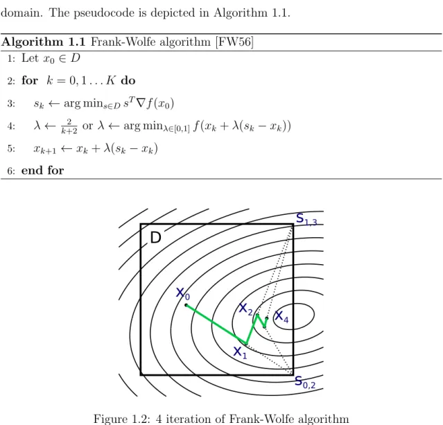
wheref(x) is a convex and continuously differentiable. Dis a compact optimization domain. The pseudocode is depicted in Algorithm 1.1.

Algorithm 1.1 Frank-Wolfe algorithm [FW56] 1: Letx0 ∈D 2: for k = 0,1. . . K do 3: sk ←arg mins∈DsT∇f(x0) 4: λ← 2 k+2 orλ ←arg minλ∈[0,1]f(xk+λ(sk−xk)) 5: xk+1 ←xk+λ(sk−xk) 6: end for

x

₀

s

_0,2

x

₁

x

₂

s

_1,3

x

4

D

Figure 1.2: 4 iteration of Frank-Wolfe algorithm

In the line number 1 the starting point (initial solution) is chosen. A search direction is calculated in line 3. λ is a step of the algorithm in the search direction (line 4). There are two methods for determining λ. The first method, which was published in the original article [FW56], is considered to be easier for use. The second method provides better results, but the implementation is considered as the harder one.

In Figure 1.2 there is a graphical visualization. The algorithm has a bad con-vergence rate near the optimal solution. There are a lot of methods for solving this problem (e.g PARTAN FWA).

(16)

Chapter 2 Problem formulation and State of

the Art

Mathematical formulation of the problems and existing solutions are going to be described in this chapter.

The first Section contains the problem formulation of two basic traffic assignment methods (all-or-nothing and Wardrop’s equilibrium) and existing approaches for solving problems, that relate to these methods.

Problem formulation and existing methods for the matrix estimation are de-scribed in the second section of this chapter.

2.1 Traffic assignment

Traffic assignment is a process which assigns the traffic volume for every road link in the network. The input is the ODM and the output is the number of vehicles that crosses the link.

The upcoming text describes the two methods of assignment (all-or-nothing and equilibrium). In this thesis we focus on the implementation of the approach with no congestion effects. The reason is that the congestion effect is insignificant for a large area of the interest (a main road and first-third class road between the cities), that we focus on.

(17)

2.1.1 All-or-nothing method

This method ignores the congestion effect, which means that every link in the net-work has a fixed travel cost. Mathematical model for the traffic volume (va) at link a∈A is va= X i X j Tijδija (2.1)

where T is the ODM and δ_ija is defined as:

δ_ija =     

1 if path from i to j crosses edge a

0 else

(2.2)

The functionδ_ija is determined by using a general algorithm for the shortest path search (e.g Dijkstra, Floyd–Warshall). This method is sensitive to the path choice, so it is necessarily to choose carefully the weight of the edges in the network. The cost of the edge is a linear combination of the length and usual travel time usually (called generalized cost).

This method is suitable for the uncongested networks (macroscopic networks).

2.1.2 Wardrop’s method

Wardrop’s assignment method reflects the congestion effect. The travel cost is con-sidered as a function of the traffic volume. This dependence is expressed as a Cost-flow curves (Ca).

Ca=Ca(va) (2.3)

Most commonly, the function is determined by using a road capacity (vehicles per hour).

The equilibrium state is searched. It means that all used paths (r) from source to destination zone have the same (minimal) travel cost and unused paths have higher costs [War52].

The mathematical programming approach can be written as [BMW56]: min Tijr X a∈A Z va 0 Ca(υ)dυ (2.4)

(18)

subject to

X r

Tijr =Tij (2.5)

Tijr ≥0 (2.6)

where Tijr is the number of the trips fromi to j by pathr.

There are several methods for solving this problem. The existing approaches are [dDOW11]:

• The Frank–Wolfe Algorithm - it was the first algorithm for solving this prob-lem, but is considered as being too slow.

• Route Based Assignment - this algorithm is faster than FWA, but it needs a lot of memory [JTPR94].

• Origin Based Assignment - the latest relevant method which has an excellent convergence performance [BG02].

2.2 Origin-Destination Matrix Estimation

Origin-Destination matrix estimation is the most important step out of the four-step classic model. The ODM estimation has the main influence on the accuracy of the resulting traffic volume.

There are three basic methods of the ODM estimation [DB05]: 1) accuracy transport data survey (license plate, roadside),

2) using trip distribution model (e.g Gravity, Gravity-Opportunity), 3) calibration of existing ODM the using traffic volume counts.

The first method is the most accurate, but it is expensive and impracticable for the large area of interest.

The second method uses a trip distribution model (deterrence function). Detailed socio-economic data and information about local habits (e.g how far people travel to work) for the area of interest are needed for this second method (more in section 1.2.1).

(19)

The last method calibrates existing ODM (a target ODM) only. The target ODM can be determined using the trip distribution model. For such a purpose, less accurate statistical data are usually sufficient as its impact on the final model is insignificant (e.g only number of people in the zone).

In this chapter a following notation will be used: T Origin-Destination matrix, Tij trips between zone i and j, Oi number of trips started in zone i, Dj number of trips ends in zone j, Z set of zones.

In some cases it is easier to write equations in a vector form (bold characters are further used to represent a vector). For example, the ODM as matrix and as a vector are T =   0 10 10 0   T=         0 10 10 0         (2.7)

2.2.1 Trip Distribution model

Trip distribution model determines the number of the trips between zone i and j. The number of the trips is

Tij =OiDjAiBjfij (2.8) subject to X j Tij =Oi (2.9) X i Tij =Dj (2.10)

Ai and Bj are balancing factors. These factors can be determined according to the

Equation 2.10 and 2.9. Most commonly, iterative proportional fitting are used for this purpose.

Oi represents the number of trips starts in zone i and Dj represents the number

(20)

f is a generalized function of the travel costs (deterrence function). There are a lot of versions of this function available in the literature. For example from [dDOW11]: classic f(cij) =c−ij2 power function f(cij) =cαij exponential f(cij) =e−βcij combined function f(cij) =cαije −βcij

In practice, these parameters are usually determined empirically by a domain expert or using an accurate research in the area of interest. This method features high complexity and its application is usually highly time-expensive.

The second approach published by [TW89] uses traffic count in the road network. The relationship between model traffic and the zones by [TW89] can be expressed as follows: va = X p X i X j Op_iDp_jAp_iB_jpf_ijpδa_ij (2.11)

wherevarepresents the model traffic on linka∈A,pis a trip purpose (e.g shopping,

sports, hobbies) and δa

ij is defined as: δ_ija =     

1 if path from i to j crosses edge a

0 else

(2.12)

There is one set of parameters for every trip purpose, so for 2 parameters per function there are 2p unknown parameters. Tamin and Willumsen used non-linear-least-squares, weighted-non-linear-least-squares and maximum likelihood for determining the parameters of the deterrence function. Newton’s method was used for solving the optimization problem.

2.2.2 Using link count

This method calibrates existing ODM using the traffic counts. The traffic counts are measured values on suitable links in the road network. Input is the target ODM and output is the calibrated ODM.

(21)

The problem can be formulated as optimization of an objective function [LP08]: F(v, T) = γ1F1(T,Tb) +γ2F2(v,bv) (2.13) subject to

Tij, va ≥0 (2.14)

v =assign(T) (2.15)

whereF1andF2is distance measures,bv is vector of the traffic counts,Tbis the target ODM. assign(T) is the assignment function (one of method from chapter 2.1).

There are a lot of methods for solving this problem available in the literature. These methods can be split to 3 categories [Abr98], [BR11]:

• Information Minimization (IM) and Entropy Maximization (EM),

• Statistical approach

– Maximum likelihood,

– Generalized least squares,

– Bayesian Inference,

• Gradient based solution.

IM and EM are based on a statistical principle of maximum entropy (information entropy). The entropy function can be explicitly written as:

I =X ij Tijlog Tij c Tij ! (2.16)

The function (I) corresponds withF1 in Equation 2.13 (more in [VZW80], [vZB82]).

Maximum likelihood approach maximizes likelihood of observing ODM and the traffic counts. The likelihood can be written as:

L(T ,b b

v|T) = L(Tb|T) L( b

v|T) (2.17)

where Lis the likelihood. This equation can be rewritten according to 2.13 as

log(L(T ,b b

v|T)) = log(L(Tb|T)) +log(L( b

(22)

The functionsF1 and F2 can be defined by using a Poisson probability distribution as [Spi87] F1 =lnL(T ,b _bv|T) = X ij (−αiTij +Tbijln(αiTij)) (2.19) F2 =lnL(bv|v(T)) = X a∈Ab (_bvaln(va(T))−va(T)) (2.20) where αi = P jTb_ij P jTij (2.21) The objective functionF should be maximized by the appropriate algorithm.

The Generalized least squares is a technique similar to classic linear least squares (e.g regression). The problem can be formulated (in vector form) as [Cas84]:

arg min T ( b T−T)0Y−1(Tb −T) + ( b v−v(T))0W−1(_bv−v(T)) (2.22) whereTis the ODM as a vector,Y andW are covariance matrices andv,v_b are the traffic volumes as vectors. This method is not suitable for large models, because the matrix inversion about size |Z|2 _{takes a lot of time.}

The Bayesian Inference approach is based on Bayes theorem which provides a method for combining two source of information [Abr98], [BR11]. More information are mentioned by [Mah83] and [DF94].

The Gradient based solution (Bi-level programing approach) is the most general optimization approach, which is suitable for the large networks. The target ODM is adjusted in each iteration using suitable numerical method. A starting point for numerical minimization is the target ODM. Solution (ODM) should converge to local minimum. The minimization problem is formulated as [LP08]:

min

Tij≥0

F(T) = γ1F1(T,Tb) +γ₂F₂(v(T), b

v) (2.23)

Gradient-based descent algorithm is used usually for this minimization. Lund-gren and Peterson deeply elaborate this problem in [LP08]. Solutions based on articles [Spi90], [DB05] are going to be described in Sections 3.2 and 3.3.

(23)

Chapter 3 Formulation of Implemented

methods

This chapter presents a mathematical formulation of implemented methods for the ODM estimation and an adjustment of the existing solution for the distributed parallel environment. Furthermore, the focus was given on usage of better methods of numerical minimization.

3.1 Estimation parameters of deterrence function

This section describes the method of determining the deterrence function parame-ters. The proposed method is derived from [TW89] with some adjustments.

Used simplified approach has only one trip purpose (p = 1). Therefore, the fundamental equation can be written as

va= X i X j kOiDjAiBjfijδija (3.1) where f(cij) = cαije −βcij _(3.2)

the factorsAi and Bj were determined form Equations

Oi = X

j

(24)

Dj = X

i

OiDjAiBjfij (3.4)

The balancing factors (Ai and Bj) were determined by using the iteration

algo-rithm. The first approximation of the ODM is computed using Ai =Bj = 1. After

that, coefficientsAi are determined by using 3.3 and every matrix row is multiplied

by these coefficients. Thereafter, values Bj can be determined by using 3.4. The

last two steps are repeated until the error is small enough.

In Equation 3.1 there are 3 unknown parameters (α, β, k). These parameters must be optimized. The least square method was used for this purpose. The problem can be written as:

min α,β,k X a∈Ab (va−bva) 2 (3.5)

where _bva is the reference traffic volume (counts) in edge a ∈ Ab. A regular simplex minimization method was used for solving the problem, because the derivation Ai

and Bj byα and β is complicated and the simplex minimization is a method of the

first order so does not need the derivation.

The efficiency of all numerical methods are given by initial point choice. There-fore, the initial solution must be determined appropriately.

The initialization value of the parameterk is estimated by using the least square method 3.5 in used approach, because the explicit equation can be expressed un-like the parameters α and β that are constant in this case (minimization in one dimension). The parameterk can be expressed as:

k= P abvav 0 a P av 02 a (3.6) where v_a0 is the derivation by k:

dva dk =v 0 a= X i X j OiDjAiBjfijδaij (3.7)

3.2 Calibration method based on Spiess’s approach

A method by Spiess calibrates (estimates) the ODM by using the steepest descent. Spiess supposes that the assignment is the Wardrop’s equilibrium assignment. In this case the drivers use k paths with equal travel cost between pair of zones. The

(25)

all-or-nothing assignment method is used for our purpose. Therefore, the mathe-matical model had to be modified. This modified model is described in the following paragraphs.

The objective function can be written as [Spi90]: F(T) = 1 2 X a∈Ab (va−bva) 2 _(3.8)

where Ab⊂ A. The subset Abcontains the links, which have got the reference value of the traffic volume (links with traffic counts). According to Equation 2.13, the parameter γ1 is 0 andγ2 is 1.

A method of the steepest descent is one of the classic method for minimization. The algorithm can be written as:

xn+1 =xn−λn∇F(xn) (3.9)

where −∇F(xn) is a direction of the biggest descent and the linear coefficient λn

is a step for n-th iteration. The coefficient λn is chosen as a sufficiently small

value (classic steepest descent) or is determined by using minimization in the search direction (steepest descent with long step). Spiess used the second method (with long step) in his work. One iteration of the optimization algorithm is composed of three steps, which are:

1) determining the search direction,

2) searching minimum of the objective function in the search direction (line search),

3) updating the target ODM.

In the upcoming text gradient of the objective function F(T) are going to be used in many equations. So the gradient is:

∂F(T) ∂Tij

=X

a∈Ab

δa_ij(va−bva) (3.10)

The modeled values of the traffic volume va are calculated according to Equation

(26)

observed and the modeled traffic volume on the path between the pair of zones (from i to j). It follows that if there is no count profile on the path, the derivation is 0. Therefore OD pairs without the reference value are not calibrated. It is the main disadvantage of the approach by [Spi90]. This problem can be eliminated by using the appropriate distribution of the count profiles in the network.

x

0 x

Figure 3.1: Steepest descent with long step (green line) and Conjugate gradient method (red line) [Wik17]

There are a lot of methods for determining the search direction available in literature. The main measure of a performance is a convergence rate (speed).

Search direction as a negative value of the gradient

The simplest approach computes the search direction as a negative value of the gradient (−∇F(T)). In this case the convergence rate is poor, because the zig-zag effect occurs. This effect is significant in a narrow valley (Figure 3.1). The search direction as a negative value of the gradient was used by [Spi90].

Search direction using Conjugate gradient method

The Conjugate gradient method provides a better approach for determining the search direction. This technique was developed for solving of a big system of a linear equations. In Figure 3.1 there is a comparison of the conjugate gradient

(27)

with the method of the steepest descent. The example is in two-dimensional space. The method of the steepest descent (green line) converges to the minimum and the conjugate gradient method finds the exact minimum after 2 steps.

It can be proved that the method reaches the exact minimum of a quadratic problem after n steps, where n is a space dimension. The search direction can be written by using the conjugate gradient method as:

dk=gk+βkdk−1 (3.11)

wheredk is the search direction andgk =∇F(Tk). The linear coefficientβk can be

determined using several techniques. For example, Fletcher–Reeves [FR64]: βk = gT kgk gT k−1gk−1 (3.12) or Polak–Ribi`ere [PR69]: βk= (gk−gk−1)Tgk gT k−1gk−1 (3.13) method can be used.

The Conjugate gradient method depends on the vectors gk−1 and dk−1, therefore

requires more memory then the method of the steepest descent.

Now the target ODM can be updated using the search direction as [Spi90] T_ijk+1 =T_ijk 1−λkdk_ij (3.14) where λk is determined using a minimization of the subproblem, which is defined as:

min

λ F(Tk(1−λkdk)) (3.15)

subject to

λkdij ≤1 (3.16)

This subproblem has an analytical solution as [Spi90] λ∗ = P a∈Abv 0 a(bva−va) P a∈Abv 0 a 2 (3.17) where v_a0 = dva dλ =− X ij Tijdijδaij (3.18)

The coefficient λ∗ must be bounded according to Equation 3.16. Details about implementation in the distributed environment are contained in chapter 4.

(28)

3.3 Calibration method based on Doblas’s approach

This approach aims to improve the properties of the method according to [Spi90]. This method solves partly the problem with 0 derivation by the OD pairs (Tij)

without the count profiles (more information in section 3.2). It turned out that this method solves the problem very marginally. However, this approach will be described, because this method uses more information from the ODM (eg. sum of all trips) and the optimization process is more under control.

The minimization problem is formulated as [DB05]

min T F(T) = X a∈Ab (va−bva) 2 (3.19) subject to lij ≤Tij ≤uij (3.20) l_iO ≤X j Tij ≤uOi (3.21) lD_j ≤X i Tij ≤uDj (3.22) l ≤X ij Tij ≤u (3.23)

The biggest advantage of this algorithm is that the lower and upper bounds for every OD pair (lij, uij), sum by columns (liO, uOi ) and rows (lDj , uDj ) and for total

number of trips in the network (l, u) can be defined.

An Augmented Lagrangian Function (ALF) is used for solving the problem 3.19. The ALF is optimized by the Frank-Wolfe algorithm (FWA). The conditions 3.21, 3.22, 3.23 are solved using the ALM and condition 3.20 is tackled by the Frank-Wolfe algorithm. The Lagrangian function can be written according to [RRR06] as

(29)

[DB05] min T P(T, σ (s)_{, β}(s)_{) =}X a∈Ab (va−_bva)2 +S   X i ( uOi − X j Tij+σ O(s) i 2 −σ_iO(s) 2) +X i ( X j Tij−liO+β O(s) i 2 −β_i0(s) 2)   +S   X j ( uD_j −X i Tij+σ D(s) j 2 −σ_jD(s) 2) +X j ( X i Tij−lDj +β D(s) j 2 −βD_j (s) 2)   +S   ( u−X ij Tij+σ(s) 2 −σ(s) 2) + ( X ij Tij−l+β(s) 2 −β(s) 2)   (3.24)

where vector σ is associated with the upper bounds and β with the lower bounds. Parameter S is a scale factor, which sets an importance of a restriction part of the Lagrangian function (last 3 rows in Equation 3.24). If the scale factor is too large, the optimization is very slow and if the factor is too small, the conditions (3.21, 3.22, 3.23) are not respected. This minimization 3.24 represents one subproblem (s) of the problem 3.19.

Operator h.iis defined as:

hxi=      x for x <0 0 for x≥0 (3.25)

After the minimization the parameters of the ALF (σ and β) are updated as:

σ(_is+1) =DuO_i −X j T_ij(s)+σ_i0(s)E, β_i(s+1) =D X j T_ij(s)−l_iO+β_i0(s)E σ(_js+1) =DuO_j −X i T_ij(s)+σ_jD(s)E, β_j(s+1) =D X i T_ij(s)−l_jD +β_jD(s)E σ(s+1) =Du−X ij T_ij(s)+σ(s)E, β(s+1)=D X ij T_ij(s)−l+β(s)E (3.26) The Lagrangian function P with new parameters, that was determined by using Equations 3.26, is minimized again. The number of subproblems (iterations) is dependent on the desired accuracy.

(30)

A lot of equations by [DB05] were modified, because the all-or-nothing assign-ment is used in our approach. The modifications are similar as in previous section.

(31)

Chapter 4 Implementation

This chapter describes an implementation of the methods used or mentioned in the previous chapter and the data structures for these purposes. This entire solution is implemented by using the Apache Spark framework, which is going to be introduced in the upcoming section.

The result is a newly designed library named Spark Traffic Modeler, which ar-chitecture and interface are going to be define. The source code and documentation are published on GitHub under an open source license. The project home page can be found onhttps://github.com/kolovsky/spark-traffic-modeler.

4.1 Apache Spark

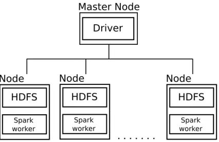
The Apache Spark is a framework for large-scale data processing, which priority is generality and speed. Spark’s abstraction is a distributed collection of data called the Resilient Distributed Dataset (RDD), which is stored across all the cluster. The RDD can be created from other technologies focused on distributed storage as file systems or databases [Spa].

In the Spark cluster, there are two basic types of nodes. The worker node pro-cesses tasks and the master node manages workers and splits the work. In each physical cluster node (computer) there are the workers and data nodes. The pro-gram can load the data from the data nodes of some distributed file system (e.g HDFS) or distributed databases (e.g Cassandra, HBase). This architecture

(32)

mini-HDFS Spark worker Node HDFS Spark worker Node Master Node Driver HDFS Spark worker Node

Figure 4.1: Schema of Apache Spark cluster

mizes the transfer between the cluster nodes because the data are processed in the same computer as are stored. In Figure 4.1 you can see the schema of the Spark cluster [Spa].

In Figure 4.2 there is a source code for the example from section 1.5. The code is written in Scala programming language, which combines the object-oriented pro-gramming with functional and runs on Java Virtual Machine (JVM). This language was chosen because Spark itself is written in Scala and Java library can be used. Spark also supports Java, Python and R.

// load text file form HDFS

val lines = sc.textFile("text.txt")

// computed mumber of word in text file using "_"

val num_of_word = lines.map(_.split().length).reduce(_+_) // same using "=>"

val num_of_word = lines.map(line => line.split().length).reduce((a,b) => a + b)

(33)

4.2 Network and graph algorithms

An important part is a model of the road network, therefore a large part of this work are graph data structures and algorithms which are customised for the use in the distributed environment.

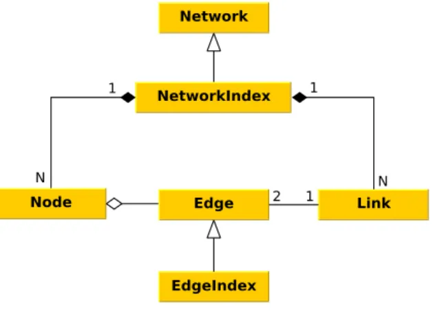
Each object must be serializable for use in the Apache Spark. Therefore, the implementation of the road network had to meet this criterion. There are many Java libraries providing the graph structures and the algorithms but did not meet the required criteria such as speed or possibility to serialize the model objects. Therefore, the implementation of the graph structure was written specifically for our purposes. Network NetworkIndex Edge Node EdgeIndex Link N N 1 2 1 1

Figure 4.3: UML digram of Network class

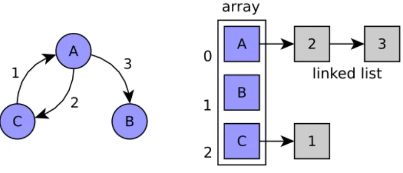
The class Network provides a functionality associated with the paths searching and other graph algorithms. The graph was implemented as an adjacency list. In Figure 4.3 you can see UML diagram of this implementation and in Figure 4.4 there is an example of the graph representation as the adjacency list. The class Graph is written as an immutable collection because it is not necessary to add any elements to the graph during the program execution.

Abstract class Network has these basic methods: addEdges,getPaths,getCosts. The method addEdges creates the graph from a list of the edges. The other two methods are the search methods that use Dijkstra’s algorithm for searching the shortest paths and the shortest distances.

(34)

A B C 1 2 3 A B C 3 2 1 array 0 1 2 linked list

Figure 4.4: Example of adjacency list representation

The conversion between the node ID and the index in the nodes array is provided by method idToNode which uses a classic Hash table.

Both direction road links were represented as two one-directional edges, but the relationship between these two edges was lost. Therefore, the class Link was added to the graph structure. Class Link provides the relationship between the edges and contains information about the travel time, the length and the link ID. In Figure 4.5 there is displayed the relationship between the Edge and Link classes.

Link Edge Edge B A A B in direction edge opposite direction edge

Figure 4.5: Relationship between class Edge and Link

4.2.1 Network optimization

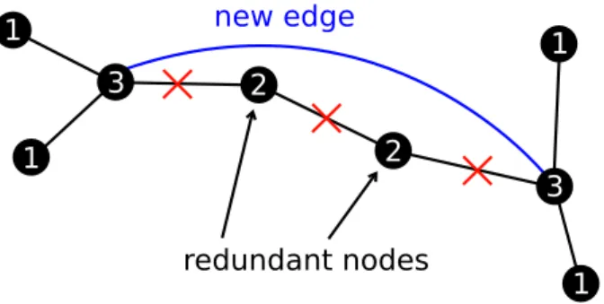
In a real road network dataset (e.g from OpenStreetMap) there are a lot of road classes as highways, sidewalks, local roads, main roads and other, however, some of them are not relevant to the transport modeling. If only the main roads are selected, the graph contains a lot of vertices with degree 2 (Figure 4.6).

(35)

1 1 1 1 3 3 2 2 redundant nodes new edge

Figure 4.6: Replacement of redundant edges by new aggregate edge

This problem was solved by an algorithm, which replaces the redundant edges by a new aggregated edge. The algorithm is based on Depth-first search (DFS). Let E is set of edges, which will be merged in one edge. In each DFS step, the algorithm detects the degree of the vertex and if the degree is 2, the edges around the vertex are added to the set E. The cost of the new edge is a sum of all edges in the set E. After that set E is set to empty. In Algorithm 4.1 there is a pseudocode of this algorithm.

This procedure reduces the number of the edges and nodes in all network, there-fore all the other graph algorithms (e.g Dijkstra) are faster.

For example, the Europe road network from OpenStreetMap (with all paths and predestinations) has about 100 mil. edges. If all the edges from the first to the third class (including motorway) are selected, the network has about 14 mil. edges and after the optimization has about 5 mil. edges. The table below shows the exact number of the edges before and after the optimization.

Europe only first 3 class after optimization 84 398 263 13 978 425 4 946 493

4.3 Framework architecture

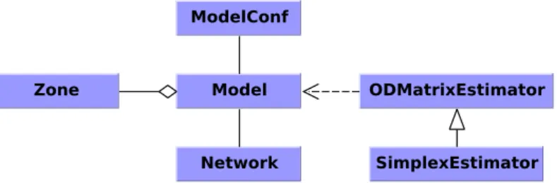
The core of the developed framework is a class Model, which provides all methods for the trip distribution, ODM calibration and for the traffic assignment (excluding the simplex algorithm). TheModelconsists of the network and the set of the zones. In Figure 4.7 you can see the framework UML diagram.

(36)

Algorithm 4.1 Graph optimization s ←some vertex from V

Let S be a stack Let set E is empty

Let function P returns previous vertex

S.push(s)

while S in not empty do

n←S.pop()

if n is not found then

n is found

for all neighborsv of n do

S.push(v) if degree ofn is 2 then if E is empty then add edge (P(n), n) to E end if add edge (n, v) to E

if degree of v is not 2 and E is not empty then

merge all edge ∈E and new edge add to graph E is empty end if end if end for end if end while

(37)

Model ModelConf ODMatrixEstimator SimplexEstimator Network Zone

Figure 4.7: Framework UML diagram

The class SimplexEstimator provides a functionality for the calibration of the deterrence function using the simplex algorithm (more in Section 3.1). This class is dependent on the classModel.

The class ModelConf is a kind of settings class, which provides the model con-stants and other model properties (e.g type of the deterrence function, max search radius for Dijkstra’s algorithm).

The class Zone represents the real zone in the model and has these properties: nearest node ID in the network, the number of trips and zone ID. Class Network

was described in Section 4.2.

The detailed description of all methods is in the documentation.

4.4 Basic parallelization technique

This section describes a technique for rewriting a mathematical formulation to the Map-Reduce programming model, which requires a different programming mindset. All-or-nothing Map-Reduce traffic assignment algorithm is going to be described. All other algorithms are based on this technique.

Reduce

Map

Figure 4.8: All-or-nothing math model with highlights Map and Reduce parts

In Figure 4.8 in Section 2.1.1 there is a traffic assignment mathematical model. Generally aggregate functions (e.g sum, min, max, std) are a Reduce type functions

(38)

(red color in Fig. 4.8). Expressions in the sum (or other aggregate function) are a Map type functions (green color).

The function δa

ij must be computed by using some shortest path search.

Dijk-stra’s algorithm was used in our case.

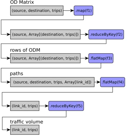
In Figure 4.9 there is an activity diagram of the traffic volume calculation. The input is the ODM, which is stored as RDD of the OD pairs (Scala data typeTuple). The output represents RDD of the traffic volumes.

(source, destination, trips)

.atMap(f3) .reduceByKey(f2) (source, Array[(destination, trips)])

.map(f1)

(source, Array[(destination, trips)])

(source, destination, trips, Array[link_id]) .atMap(f4)

(link_id, trips) .reduceByKey(f5)

(link_id, trips)

OD Matrix

rows of ODM

paths

trac volume

Figure 4.9: calculation flow of the all-or-nothing traffic assignment

In line 1 the ODM is transformed to a form which is suitable for the reduce func-tion. The functionf1transforms the Origin-Destination pair(source, destination,

trips) to a key-value form, where the key represents the source zone and the value

is an array with one item (source, Array[(destination, trips)]).

The aggregation by the source zone using thereduceByKeymethod is performed in the next line. The result of this transformation are rows of the ODM ( a key is the source zone and the value is the array of the destination zone with the number

(39)

// transform to rows form

var traffic_volume = odm.map(od => (od._1,Array((od._2, od._3)))) .reduceByKey(_++_)

// compute shortest path tree

.flatMap(row => n.getPathsTrips(row._1,row._2, m_conf.length_coef, m_conf.time_coef, Double.PositiveInfinity))

.flatMap(path => path._4.map(link_id => (link_id, path._3))) .reduceByKey(_+_)

Figure 4.10: Scala source code for all-or-nothing traffic assignment

of trips).

The function f3 at line 3 computes the shortest paths from the source zone to

all destination zones in a parameter array. All rows of the ODM are transformed to an OD pairs with a path attribute(source, destination, trips, path), where the path is an array of the link ID.

The function f4 transforms the path from the previous step to key-value pair,

where the key is a link ID and the value is the number of the trips. The last line sums the traffic volume across all paths by a link ID.

In Figure 4.10 there is entire source code. The source code is written in Scala programming language (is used the short form for function).

The same idea of programming was used for all other methods that are imple-mented in developed framework.

(40)

Chapter 5 Results

This chapter contains the test results of implemented algorithms, that was described in the previous chapter. The tests were conducted on various sizes of the road network with a different number of zones from a relatively small model (model of country region) to a large scale model (model of whole Europe). The real application of the developed framework is described at the end of this chapter.

5.1 Hardware and datasets for testing

Three datasets were created for testing our framework. In Table 5.1 there are parameters of these datasets, where the counts represent the values of the reference traffic volume.

The model of Pilsen is small-sized and was used primarily for the development because all algorithms take less time to compute this model. The second model represents the Czech republic. The set of all zones contains every village and all city district. The road network consists of each road, including all streets. The last model covers all Europe. It includes all roads from motorways to 3rd class. LAU 2 (Local Administrative Units) according to Europe Union (EU) represent the set of the zones.

Testing was realized on two types of hardware. The dataset City of Pilsen was tested on a laptop (Intel(R) Core(TM) i5-4300M CPU @ 2.60GHz, 8GB RAM). The other two models were calculated on the cluster, which runs in YARN mode and

(41)

Name number of edges number of zones number of counts

City of Pilsen 12 207 115 60

Czech Republic (CR) 2 596 030 22 492 6 407

Europe 4 946 493 156 812 6 381

Table 5.1: Datasets for testing

has 24 nodes. Every node contains 16 cores (Intel(R) Xeon(R) CPU E5-2630 v3 @ 2.40GHz) and has 128 GB RAM. So the program can use 3TB of memory and 384 cores.

5.2 Trip distribution

Two methods for the initial estimation of the ODM were implemented. These meth-ods are:

• using the model from Section 3.1, where the parameter k is estimated by the least squares method

• using the same model, where all parameters are estimated by a simplex method The second approach is not suitable for the large models because its computational complexity is high. This method was tested only on the City of Pilsen dataset. The first method, where the parameterkis estimated, showed that the initial ODM can be computed in an acceptable time. Therefore, this approach was used for the testing. In Table 5.2 there is an uptime for all models. The uptime includes the time for data loading too. The ODM size represents the number of the OD pair (number of cell in the ODM).

In this case, 4 cores and 32 GB of memory per node were used in the cluster (96 cores in total).

(42)

dataset uptime ODM size note City of Pilsen < 5 s 10 302 localhost

CR 41 min 421 686 118

Europe 1.6 h 829 051 938 search radius was set to 200 km Table 5.2: Trip distribution test

5.2.1 Calibration

Two methods for the ODM calibration using traffic count were implemented. These methods are base on

• Spiess’s approach (more in Section 3.2) and

• Doblas’s approach (more in Section 3.3).

The first method based on Spiess’s approach can be divided according to used algorithm for the numerical minimization of the objective function F. These algo-rithms are:

• the steepest descent with long step,

• conjugate gradient method by Fletcher–Reeves,

• conjugate gradient method by Polak–Ribi`ere.

The tests showed that the second method by Doblas is not suitable for the large models because the convergence rate is not satisfactory and the algorithm needs a lot of parameters, that must be set very precisely (e.g the scale parameter S). Therefore, this method was not used for the final performance testing.

The convergence test was performed for the three algorithms, that were used for the minimization of the function F(T) in the method by Spiess. This test runs on the laptop, which is described in the text above. The City of Pilsen dataset was used. All three algorithms take approximately the same time. The steepest descent takes 14 s. Fletcher–Reeves and Polak–Ribi`ere takes 15 s. In Figure 5.1 there is the convergence rate for all these minimization algorithms.

(43)

0 5 10 15 20 25 30 35 0 100 200 300 400 500 600 steepest descent Polak–Ribière Fletcher–Reeves iInu number of iterations standard deviation [vehi cles per ho ur]

Figure 5.1: convergence rate for the implemented minimization algorithms

The Polak–Ribi`ere method gives the best result as expected. Therefore, this approach was used for the calibration of the ODM for the Europe model.

Furthermore, the application uptime was measured depending on the number of computing nodes. In this case, only one iteration of the Polak–Ribi`ere method was performed on the Czech republic model. It follows that all shortest paths between the zones are computed. Further, one step of the conjugate gradient method is performed.

This test was performed on the cluster, where 24, 18, 12, 6 and 3 nodes (workers) were used (96, 72, 48, 24 and 12 cores). In Figure 5.2 there is speed-up and the application uptime, that are dependent on the number of the computing nodes used in the cluster. The application uptime includes a time for data loading. The input matrix is stored across 24 nodes. Therefore, if the application uses less nodes, the parts of the matrix that are stored in the unused nodes, must be moved to the active nodes.

dataset uptime ODM size iteration note

City of Pilsen < 15 s 10 302 30 localhost using 1 core

CR 6 h 421 686 118 20

Europe 31.1 h 829 051 938 30 search radius was set 200 km Table 5.3: Application uptime of the ODM calibration

(44)

0 5 10 15 20 25 30 0 1 2 3 4 5 6 7 8 number of workers speed-up

workers cores uptime [h]

3 12 6.95

6 24 3.26

12 48 2.27

18 72 1.11

24 96 0.94

Figure 5.2: Application uptime dependent on the number of computing nodes

In Figure 5.3 there is application uptime of the ODM calibration for all datasets. The conjugate gradient method together with Polak–Ribi`ere method for determining the search direction were used for these tests. In this case, 4 cores and 32 GB of memory per node were used in the cluster.

5.3 Traffic assignment

The last test that was conducted, is the all-or-nothing traffic assignment which was described in detail in Section 4.4. The whole source code in Scala of this method is presented in Figure 4.10. This test was performed on the same cluster configuration as in the previous section (96 cores).

dataset uptime ODM size note

City of Pilsen < 2.5 s 10 302 localhost using 1 core

CR 1.3 h 421 686 118

Europe 2.3 h 829 051 938 search radius was set to 200 km Table 5.4: Application uptime of all-or-nothing traffic assignment

5.4 Practical example

The developed framework (Spark traffic modeler) was used for the creation of the European transport model. The transport model includes all motorways and 1-3

(45)

classes of roads. LAU 2 (Local Administrative Units level 2) were used as the zones. Areas (LAU2), which were too large, were split to the more zones (e.g big cities). More about the process of developing a set of the zones can be found in (more in [JHJ+_17]).

Values of the traffic volume for the mentioned roads were calculated by using this model. The initial ODM was estimated by using the method, which estimates the parameter k of the deterrence function using the least square method (more in Section 3.1). The standard deviation of the initial ODM was around 15 000 vehicles per day. The conjugate gradient method was used for the calibration, where the search direction was determined by using the Polak-Ribiere method. This method reduced the standard deviation to 3300 vehicles per day after 30 iterations. The all-or-nothing method was used for the traffic assignment.

The cluster configuration was the same as with the last test (24 x 4 cores). The entire calculation took about 35 hours. The calculated traffic volumes have been added to OpenTransportMap (http://opentransportmap.info/), which originated in the European project OpenTransportNet (http://opentnet.eu/) (more in [JHJ+_]).

OpenTransportMap is open dataset for the transport application, which is compat-ible to INSPIRE Transport Network.

In Figure 5.3a there is a visualization of the zones, where the dot size is based on the number of the trips in the zone. The second Figure 5.3b depicts the visualization of the values of the traffic volumes. Green color means small values and red color represents big values of the traffic volumes.

5.5 Lessons learned

Apache Spark is a young computer system compared to relational databases. There-fore, this section has been included to the thesis.

During the implementation, we came across the problems, that can be split into memory and cache problems.

Spark starts to compute after the last command in a job (spark is ”lazy”). It means, that any sub-result does not physically exist. In example from previous

(46)

(a) Zones (b) T raffic v ol ume s Figure 5.3: Europ e transp ort mo del

(47)

lines loads le .map .reduce .count lines loads le .map .reduce .count lines loads le number of words number of words number of lines number of lines a) b)

Figure 5.4: a) withlines.persist() b) without lines.persist()

section (Figure 4.2) there is only one job. Last value (num of word) exists in memory only. If the variable lines is used in other job (e.g we want to compute a number of the lineslines.count()), Spark performs again all previous calculations (in this case loads data from the disk). Finally Spark loads all data from the disk twice. It follows that Spark remembers the calculation procedure.

These properties are not suitable for the iteration algorithms because the calcu-lation history is very long and without caching all previous results are calculated in every iteration. In Figure 5.4 you can see the calculation procedure with and without caching.

For caching there is a method of the RDD named persist(). The argument of the function is a storage level. The possible storage levels are:

level storage

DISK ONLY only to disk

MEMORY AND DISK memory and disk

MEMORY AND DISK SER serialized

MEMORY ONLY only in memory

MEMORY ONLY SER serialized

It is necessary to call thepersistmethod after every iteration. Furthermore, it is suitable to call method checkpoint or localCheckpoint, because the calculation history is forgotten using these methods. Then the developer has certainty that Spark uses the data from the cache and does not compute all previous results again because Spark forgot the history.

(48)

Conclusion

The aim of this work is to convert, test and evaluate the traffic volume calculation into the distributed parallel computing environment.

The review of the relevant literature about the Origin-Destination matrix estima-tion and the traffic assignment was performed. Furthermore, the existing soluestima-tions for the traffic modeling have been explored.

Our solution was designed by using the most suitable methods, which are con-tained in the state-of-the-art. The designed solution was implemented by using a framework for distributed computing Apache Spark.

The tests and benchmarking showed that the best method for ODM estimation using the traffic count for the large models is the method by [Spi90], where the conjugate gradient method, where the search direction is determined by using the Polak-Ribiere method, is used. The all-or-nothing method of the traffic assignment was implemented only, because it is enough for uncontested networks, which was used in the models.

The solution can create larger models then the standard softwares for the traffic modeling based on desktop environment and is scalable. This property was used to create the model of the whole Europe. The model contains approximately 150 000 zones and the road network has 5 000 000 links. This model was used to calculate the traffic volume for an open dataset OpenTransportMap (OTM), which is a part of the project OpenTransportNet (OTN).

In future, the algorithm for Wardrop’s equilibrium traffic assignment needs to be implemented. This is a prerequisite for creating a service for the real-time traffic assignment for the large city models.

(49)

Bibliography

[Abr98] Torgil Abrahamsson. Estimation of origin-destination matrices using traffic counts-a literature survey. 1998.

[BG02] Hillel Bar-Gera. Origin-based algorithm for the traffic assignment prob-lem. Transportation Science, 36(4):398–417, 2002.

[BMW56] Martin Beckmann, CB McGuire, and Christopher B Winsten. Studies in the economics of transportation. Technical report, 1956.

[BR11] Sharminda Bera and KV Rao. Estimation of origin-destination matrix from traffic counts: the state of the art. 2011.

[Cas84] Ennio Cascetta. Estimation of trip matrices from traffic counts and sur-vey data: a generalized least squares estimator. Transportation Research Part B: Methodological, 18(4-5):289–299, 1984.

[DB05] Javier Doblas and Francisco G Benitez. An approach to estimating and updating origin–destination matrices based upon traffic counts preserv-ing the prior structure of a survey matrix. Transportation Research Part B: Methodological, 39(7):565–591, 2005.

[dDOW11] Juan de Dios Ortuzar and Luis G. Willumsen. Modelling Transport. John Wiley & Sons, Ltd, 2011. ISBN 978-0-470-76039-0.

[DF94] Soumya S Dey and Jon D Fricker. Bayesian updating of trip gener-ation data: combining ngener-ational trip genergener-ation rates with local data.

(50)

[DG08] Jeffrey Dean and Sanjay Ghemawat. Mapreduce: simplified data pro-cessing on large clusters. Communications of the ACM, 51(1):107–113, 2008.

[Dij59] Edsger W Dijkstra. A note on two problems in connexion with graphs.

Numerische mathematik, 1(1):269–271, 1959.

[FR64] Reeves Fletcher and Colin M Reeves. Function minimization by conju-gate gradients. The computer journal, 7(2):149–154, 1964.

[FT87] Michael L Fredman and Robert Endre Tarjan. Fibonacci heaps and their uses in improved network optimization algorithms. Journal of the ACM (JACM), 34(3):596–615, 1987.

[FW56] Marguerite Frank and Philip Wolfe. An algorithm for quadratic pro-gramming. Naval research logistics quarterly, 3(1-2):95–110, 1956. [JHJ+_] _{Karel Jedliˇ}_{cka, Pavel H´}_{ajek, Jan Jeˇ}_{zek, Frantiˇsek Kolovsk´}_{y, Tom´}_aˇs

Mil-dorf, Karel Charv´at, Dmitrii Kozhukh, Jan Martolos, Jan ˇSˇtastn´y, and Daniel Beran. Open transport map: open, harmonized dataset or road network.

[JHJ+_17] _{Karel Jedliˇ}_{cka, Pavel H´}_{ajek, Jan Jeˇ}_{zek, Frantiˇsek Kolovsk´}_{y, Daniel}

Be-ran, Tomáˇs Mildorf, Karel Charvát, Dimitri Kozhukh, Jan Martolos, and Jan ˇSˇtastný. Otevˇrená dopravn´ı mapa pro evropu. GIS Ostrava, 2017.

[JTPR94] R Jayakrishnan, Wei T Tsai, Joseph N Prashker, and Subodh Rajad-hyaksha. A faster path-based algorithm for traffic assignment.University of California Transportation Center, 1994.

[LP08] Jan T Lundgren and Anders Peterson. A heuristic for the bilevel origin– destination-matrix estimation problem.Transportation Research Part B: Methodological, 42(4):339–354, 2008.

(51)

[Mah83] MJ Maher. Inferences on trip matrices from observations on link vol-umes: a bayesian statistical approach. Transportation Research Part B: Methodological, 17(6):435–447, 1983.

[PR69] Elijah Polak and Gerard Ribiere. Note sur la convergence de méthodes de directions conjuguées. Revue fran¸caise d’informatique et de recherche opérationnelle, série rouge, 3(1):35–43, 1969.

[RRR06] A Ravindran, Gintaras Victor Reklaitis, and Kenneth Martin Ragsdell.

Engineering optimization: methods and applications. John Wiley & Sons, 2006.

[Spa] Apache spark dokumentation.

[Spi87] Heinz Spiess. A maximum likelihood model for estimating origin-destination matrices. Transportation Research Part B: Methodological, 21(5):395–412, 1987.

[Spi90] Heinz Spiess. A gradient approach for the od matrix adjustment prob-lem. 1:2, 1990.

[TW89] O. Z. Tamin and L. G. Willumsen. Transport demand model estimation from traffic counts. Transportation, 16(1):3–26, 1989.

[vZB82] Henk J van Zuylen and David M Branston. Consistent link flow esti-mation from counts. Transportation Research Part B: Methodological, 16(6):473–476, 1982.

[VZW80] Henk J Van Zuylen and Luis G Willumsen. The most likely trip matrix estimated from traffic counts. Transportation Research Part B: Method-ological, 14(3):281–293, 1980.

[War52] John Glen Wardrop. Road paper. some theoretical aspects of road traffic research. Proceedings of the institution of civil engineers, 1(3):325–362, 1952.

(52)

[Wik17] Wikipedia. Conjugate gradient method — wikipedia, the free encyclo-pedia, 2017. [Online; accessed 9-May-2017].

(53)

Appendix A

Contents of attached CD

• MT Kolovsky.pdf- master thesis

• src/main/scala/com/kolovsky/traffic modeler - source code folder

– Cell.scala – Edge.scala – EdgeIndex.scala – Lagrange.scala – Link.scala – MinOrderNodeStatic.scala – Model.scala – ModelConf.scala – Network.scala – NetworkIndex.scala – Node.scala – ODMatrixEstimator.scala – ODPair.scala – SimplexEstimator.scala – Zone.scala

• readme.txt - readme file with a demonstration of use